Bad semidefinite programs: they all look the same
G´
abor Pataki
∗October 8, 2018
Abstract
Conic linear programs, among them semidefinite programs, often behave pathologically: the optimal values of the primal and dual programs may differ, and may not be attained. We present a novel analysis of these pathological behaviors. We call a conic linear system Ax≤K bbadly behavedif the value of sup{hc, xi|Ax≤K b}is finite but the dual program has no solution with the same value forsomec.We describe simple and intuitive geometric characterizations of badly behaved conic linear systems. Our main motivation is the striking similarity of badly behaved semidefinite systems in the literature; we characterize such systems by certainexcluded matrices,
which are easy to spot in all published examples.
We show how to transform semidefinite systems into a canonical form, which allows us to easily verify whether they are badly behaved. We prove several other structural results about badly behaved semidefinite systems; for example, we show that they are inN P ∩co-N P in the real number model of computing. As a byproduct, we prove that all linear maps that act on symmetric matrices can be brought into a canonical form; this canonical form allows us to easily check whether the image of the semidefinite cone under the given linear map is closed.
Key words: conic linear programming; semidefinite programming; duality; closedness of the linear image of a closed convex cone; pathological semidefinite programs
MSC 2010 subject classification: Primary: 90C46, 49N15; secondary: 52A40
OR/MS subject classification: Primary: convexity; secondary: programming-nonlinear-theory
1
Introduction
Many problems in engineering, combinatorial optimization, machine learning, and related fields can be formulated as the primal-dual pair of conic linear programs
sup hc, xi inf hb, yi
(Pc) s.t. Ax≤Kb s.t. y≥K∗0 (Dc)
A∗y=c,
∗Department of Statistics and Operations Research, University of North Carolina at Chapel Hill
where A : X → Y is a linear map between finite dimensional Euclidean spaces X and Y, A∗ is its
adjoint,K⊆Y is a closed, convex cone,K∗ is its dual cone, ands≤Kt meanst−s∈K. Note that the subscriptc refers to the objective of the primal problem.
Problems (Pc) and (Dc) generalize linear programs and share some of the duality theory of linear
programming. For instance, a pair of feasible solutions always satisfies the weak duality inequality
hc, xi ≤ hb, yi. However, in conic linear programming pathological phenomena occur: the optimal values of (Pc) and of (Dc) may differ, and they may not be attained.
In particular, semidefinite programs (SDPs) and second order conic programs (SOCPs) — probably the most useful and pervasive conic linear programs — often behave pathologically: for a variety of examples we refer to the textbooks [6, 37, 11, 3, 42] surveys [44, 41, 27] and research papers [34, 1, 43]. Pathological conic LPs are both theoretically interesting and often difficult, or impossible to solve numerically.
These pathologies arise, since the linear image of a closed convex cone is not always closed. For recent studies about when such sets are closed (or not), see e.g., [4, 2, 29]. Three approaches (which we review in detail below) can help to avoid or remedy the pathologies: one can impose a constraint qualification (CQ), such as Slater’s condition; one can regularize (Pc)-(Dc) using a facial reduction
algorithm [16, 46, 31]; or write anextended dual [34, 24], which uses extra variables and constraints. However, such CQs often do not hold, and neither facial reduction algorithms nor extended duals can help solve all pathological instances.
We started this research observing that pathological SDPs in the literature look curiously similar and one of our main goals is to find the root cause of the similarity. We focus on the system underlying (Pc) and call
Ax≤K b (P)
badly behavedif there existsc such that (Dc) either does not attain its value or its value differs from
the value of (Pc).We call (P)well behaved if it is not badly behaved.
Main contributions of the paper:
(1) In Theorem 1 of Section 2 we characterize when the system (P) is badly or well behaved. At the heart of Theorem 1 is a simple geometric condition that involves the set of feasible directions at
z∈K, i.e.,
{y|z+y∈Kfor some >0},
andz is chosen as a certainslackin (P).
In Theorem 1 we unify two well-known (and seemingly unrelated) conditions for (P) to be well behaved: the first is Slater’s condition, and the second requiresKto be polyhedral.
Theorem 1 relies on a result on the closedness of the linear image of a closed convex cone from [29] (which we recap in Lemma 1).
(2) In Section 3 we characterize when a semidefinite system
m
X
i=1
xiAiB (PSD)
is badly behaved via certain excluded matrices. We assume (with no loss of generality) that a maximum rank positive semidefinite matrix of the formB−P
ixiAi is
Z = Ir 0 0 0
!
We prove (in Theorem 2) that (PSD) is badly behaved iff there is a matrix V which is a linear combination of theAi andB of the form
V = V11 V12
VT 12 V22
!
, (1.2)
where V11 is r×r, V22 is positive semidefinite, and R(V12T) 6⊆ R(V22). Here R() stands for rangespace.
The excluded matrices Z and V are easy to spot in all published badly behaved semidefinite systems (we counted about 20 in the above references). The simplest such system is
x1
α 1 1 0
!
1 0
0 0
!
, (1.3)
whereαis any real number: in (1.3) the right hand side serves asZ and the matrix on the left hand side serves asV.
Theorem 3 similarly characterizes well behaved semidefinite systems.
Theorems 2 and 3 follow from Theorem 1, and Lemma 3, which characterizes the set of feasible directions and related sets in the semidefinite cone.
(3) How do we verify that (PSD) is badly or well behaved? In other words, how do we convince a nonexpert reader that an instance of (PSD) is badly or well behaved? Theorems 4 and 5 in Section 4 show how to transform (PSD) into an equivalent standard system, whose bad or good behavior is self-evident. The transformation is surprisingly simple, as it relies mostly on elementary row operations — the same operations that are used in Gaussian elimination. A natural analogy (and our inspiration) is how one transforms an infeasible linear system of equations Ax=b to derive the obviously infeasible equationh0, xi= 1.
Here we also prove that i) badly/well behaved semidefinite systems are inN P ∩co-N Pin the real number model of computing ii) for a well behaved semidefinite system we can restrict optimal dual matrices to be block-diagonal, and iii) roughly speaking, we can partition a well behaved system into a strictly feasible part, and a linear part.
As a byproduct, we prove that all linear maps that act on symmetric matrices can be brought into a canonical form; this canonical form allows us to easily check whether the image of the semidefinite cone under the given linear map is closed.
(4) In Section 5 we sketch analogous results for conic linear programs and SDPs in the dual form and prove that all badly behaved semidefinite systems can be reduced, by a sequence of natural operations, to the system (1.3).
(5) Since most examples in the main body of the paper have at most three variables and 3×3 matrices, in Appendix A we give a larger illustrative example with four variables and 4×4 matrices. We prove other technical results in Appendix B.
We illustrate our results by many examples. The only technical proofs in the main body of the paper are those of Theorem 1 and of Lemma 5, and these can be safely skipped at first reading.
Related work A fundamental question in convex analysis is whether the linear image of a closed convex cone is closed. In this paper we rely on Theorem 1.1 from [29], which we summmarize in Lemma 1. This result gives several necessary conditions, and exact characterizations for the class of
and to Waksman and Epelman [47] for another related result. For perturbation results we refer to Borwein and Moors [13, 14]; the latter paper shows that the set of linear maps under which the image of a closed convex cone is not closed is small both in terms of measure and category. For a more general problem, whether the intersection of an infinite sequence of nested sets is nonempty, Bertsekas and Tseng [7] gave a sufficient condition. Their characterization is in terms of a certainretractiveness
property of the set sequence.
We say that (Dc) is astrong dual of (Pc) if they have the same value, and (Dc) attains this value,
when it is finite. Thus in general (Dc) is not a strong dual of (Pc).Using this terminology, (P) is well
behaved exactly if (Dc) is a strong dual of (Pc) forallc.We say that (P) satisfiesSlater’s condition,
if there isxsuch that b− Axis in the relative interior ofK; if this condition holds, then (P) is well behaved.
Ramana in [34] proposed a strong dual for SDPs, which uses polynomially many extra variables and constraints. His result implies that semidefinite feasibility is inN P ∩co-N P in the real number model of computing. Klep and Schweighofer in [24] constructed a Ramana-type strong dual for SDPs, which, interestingly, is based on ideas from algebraic geometry, rather than from convex analysis.
The facial reduction algorithm of Borwein and Wolkowicz in [16, 15] converts (P) into a system that satisfies Slater’s condition, and is hence well behaved. The algorithm relies on a sequence of reduction steps. For more recent, simplified facial reduction algorithms, see Waki and Muramatsu [46] and Pataki [31]. Ramana, Tun¸cel, and Wolkowicz in [36] proved the correctness of Ramana’s dual from the facial reduction algorithm of [16, 15], showing the connection of these two seemingly unrelated concepts. We refer to Ramana and Freund [35] for a proof that the Lagrange dual of Ramana’s dual has the same value as the original problem. Generalizations of Ramana’s dual are known for conic LPs overnicecones [31]; and for conic LPs over homogeneous cones (P´olik and Terlaky [33]).
For a generalization of the concept of strict complementarity (a concept that plays an important role in our work), we refer to Pena and Roshchina [32]. Schurr et al in [40] characterizeuniversal duality
— when strong duality holds for all right hand sides and objective functions. Tun¸cel and Wolkowicz in [43] related the lack of strict complementarity in a homogeneous conic linear system to the existence of an objective function with a positive gap.
We finally remark that the technique of reformulating equality constrained SDPs (relying mostly on elementary row operations), to easily verify their infeasibility was used recently by Liu and Pataki [25].
1.1
Preliminaries. When is the linear image of a closed convex cone closed?
We now review some basics in convex analysis, relying mainly on references [38, 23, 12, 5]. In Lemma 1 we also give a short and transparent summary of a result on the closedness of the linear image of a closed convex cone from [29].
Ifxandy are elements of the same Euclidean space, we sometimes writex∗y forhx, yi.For a set
Cwe denote its linear span, the orthogonal complement of its linear span, its closure, and interior by linC, C⊥,clC, and intC, respectively. For a convex setC we denote its relative interior by riC.For a convex setC andx∈C we define
dir(x, C) = {y|x+y∈Cfor some >0}, (1.4) ldir(x, C) = dir(x, C)∩ −dir(x, C), (1.5) tan(x, C) = cl dir(x, C)∩ −cl dir(x, C). (1.6)
A set C is acone ifλx∈C holds for allx∈C, and λ≥0. LetC be a closed convex cone. Its dual cone is
C∗ = {y| hy, xi ≥0 ∀x∈C}.
ForE, a convex subset ofC, we say thatE is afaceofC, ifx1, x2∈C, and 1/2(x1+x2)∈E implies thatx1 andx2are in E.
For x∈C andu∈C∗, we say thatuis strictly complementary to x if u∈ri(C∗∩x⊥). IfC is the semidefinite cone, or the second order cone, thenuis strictly complementary tox iffxis strictly complementary tou; in other cones, however, this may not be the case (see a discussion in [28]).
We say that a closed convex coneC isnice, if
C∗+E⊥is closed for allEfaces of C.
We know that polyhedral, semidefinite, andp-order cones are nice [16, 15, 29]; the intersection of a nice cone with a linear subspace and the linear preimage of a nice cone are nice [18]; hence homogeneous cones are nice, as they are the intersection of a semidefinite cone with a linear subspace (see [17, 22]). In [30] we characterized nice cones, proved that they must be facially exposed and conjectured that all facially exposed cones are nice. However, Roshchina [39] disproved this conjecture.
We denote the rangespace, nullspace, and adjoint operator of a linear operatorMbyR(M),N(M) and M∗, respectively. We denote by Sn the set of n by n symmetric matrices, and by Sn
+ the set ofn×n symmetric positive semidefinite (psd) matrices. For symmetric matrices A and B we write
AB [A≺B] to denote thatB−Ais positive semidefinite [positive definite], and we writeA•B to denote the trace ofAB.We have (Sn
+)∗=S+n with respect to the• inner product. We will use the fact that for anH ⊆ Sn affine subspace
ri(H∩ Sn
+) = {X ∈ S+n|Xis a maximum rank psd matrix inH}.
ForA, B∈ Sn and an invertible matrix T we will use the identity
TTAT•T−1BT−T = A•B. (1.7)
For matricesA1 andA2, we let
A1⊕A2 =
A1 0 0 A2
!
,
and for sets of matricesX1 andX2 we define
X1⊕X2 = {A1⊕A2|A1∈X1, A2∈X2}.
For instance,Sr
+⊕{0}(where the order of the 0 matrix will be clear from context) is the set of matrices with the upper leftr×rblock positive semidefinite and the rest of the components zero.
We writeIrfor the identity matrix of orderr.
The following question is fundamental in convex analysis: when is the linear image of a closed convex cone closed? We state and illustrate a short version of Theorem 1.1 from [29], which gives easily checkable conditions which are “almost” necessary and sufficient. We will use Lemma 1 later on to prove Theorem 1.
(1) R(M)∩ cl dir(w, C)\dir(w, C)
=∅.
(2) There isw0∈ N(M∗)∩C∗ strictly complementary to w, and
R(M)∩ tan(w, C)\ldir(w, C)=∅.
Our first example which illustrates Lemma 1 is very simple:
Example 1. LetC=C∗=S2
+ and define the mapM:R2→ S2as
M(x1, x2) =
x1 x2
x2 0
!
.
Then M∗Y = (y
11,2y12)TwhereY ∈ S2, and M∗C∗ is not closed: a direct computation shows
M∗C∗= (
R++×R)∪(0,0),whereR++ stands for the set of strictly positive reals.
Lemma 1 also proves thatM∗C∗ is not closed: to see how, let
w= 1 0 0 0
!
, v= 0 1 1 0
!
.
Then w ∈ ri(R(M)∩C), since it is a maximum rank psd matrix in R(M). Also, v ∈ R(M)∩
(cl dir(w, C)\dir(w, C)), sincev6∈dir(w, C) follows from the definition, andv ∈cl dir(w, C) follows, since putting any >0 into the (2,2) position ofv makes it a feasible direction. So condition (1) of Lemma 1 is violated, henceM∗C∗ is not closed.
The next, more involved example illustrates the key point of Lemma 1: the image setM∗C∗usually
has much more complicated geometry thanCandC∗.Lemma 1 sheds light on the geometry ofM∗C∗
via the geometry of the simpler setC.
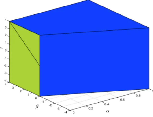
Example 2. LetC=C∗=S3
+ and define the mapM:R3→ S3as
M(x1, x2, x3) =
x1 2x2 x3 2x2 x2+x3 0
x3 0 0
.
ThusM∗Y = (y11, y22+ 4y12, y22+ 2y13), whereY ∈ S3.
It is a straightforward computation (which we omit) to show
cl(M∗C∗) = {(α, β, γ) : α≥0,4α+β ≥0},
cl(M∗C∗)\ M∗C∗ = {(0, β, γ) : γ6=β≥0}. (1.8)
The setM∗C∗ is shown on Figure 1 in blue, and cl (M∗C∗)\ M∗C∗ in green. (Note that the blue
diagonal segment on the green facet actually belongs toM∗C∗.)
Lemma 1 easily proves thatM∗C∗ is not closed, even without computing the sets in (1.8); indeed,
let
w := M(6,1,0) =
6 2 0 2 1 0 0 0 0
, v:=M(0,0,1) =
0 0 1 0 1 0 1 0 0
and observe i)w∈ri(R(M)∩C),since it is a maximum rank psd matrix inR(M); ii) v6∈dir(w, C) follows from the definition; and iii)v∈cl dir(w, C), since putting any >0 into the (3,3) position of
vmakes it a feasible direction.
Thus condition (1) in Lemma 1 is violated, soM∗C∗ is not closed.
Figure 1: The setM∗C∗ is in blue, and cl (M∗C∗)\ M∗C∗ is in green
We mention in passing that the second part of condition (2) in Lemma 1 is stated in Theorem 1.1 in [29] as R(M)∩((E4)⊥\linE) = ∅, where E is the smallest face of C that contains w and
E4=C∗∩w⊥.However, this is an equivalent formulation, as implied by the characterization of linE
and (E4)⊥, see e.g., Lemma 7 in Appendix B.
Throughout the paper we assume that (P) is feasible. Recall that we say that (P) satisfiesSlater’s conditionif there exists xsuch thatb− Ax∈riK.
2
When is a conic linear system badly or well behaved?
In this section we present our main characterization of when (P) is badly or well behaved (these concepts are defined in the Introduction). We first need a definition.
Definition 1. Aslackin (P) is a vector in
(R(A) +b)∩K,
and amaximum slackis a vector in the relative interior of all slacks.
We start with a basic lemma:
Lemma 2. The system (P) is well behaved, if and only if the set
A∗ 0 b∗ 1
!
K∗
R+
!
To put Lemma 2 into perspective, note that the image set in Lemma 2 is closed if (A, b)∗K∗ is closed (one can argue this directly or by modifying the proof of Lemma 2). In turn, if (A, b)∗K∗ is closed, then the duality gap between (Pc) and (Dc) is zero, even ifK lives in an infinite dimensional
space — see, e.g., Theorem 7.2 in [3] (where our primal is called the dual). The proof of Lemma 2 is standard, and we give it in Appendix B.
The main result of this section follows (recall the definition of dir(z, K) and related sets from (1.4)–(1.6)). We writeR(A, b) for the rangespace of the operator (x, t)→ Ax+bt.
Theorem 1. Let z be a maximum slack in (P). Conditions (1) and (2) below are equivalent to each other, andnecessary for (P) to be well behaved. IfK is nice, then they arenecessary and sufficient.
(1) R(A, b)∩(cl dir(z, K)\dir(z, K)) =∅.
(2) There isu∈ N (A, b)∗
∩K∗ strictly complementary to z, and
R(A, b)∩ tan(z, K)\ldir(z, K)
=∅.
To build intuition we show how Theorem 1 unifies two classical, seemingly unrelated, sufficient
conditions for (P) to be well-behaved.
Corollary 1. Suppose that K is a nice cone. If K is polyhedral or (P) satisfies Slater’s condition, then (P) is well-behaved.
Proof Let z be a maximum slack in (P). IfK is polyhedral, then so is dir(z, K). If (P) satisfies Slater’s condition, then clearlyz∈riK,so dir(z, K) = linK. In both cases dir(z, K) is closed, hence Condition (1) holds, so (P) is well behaved.
Though Lemma 2 is a bit simpler to state than Theorem 1, the latter will be more useful. On the one hand, Lemma 2 relies on the closedness of the linear image ofK∗×R+, which may not be easy to check. On the other hand, Theorem 1 relies on the geometry of the coneK itself, and not on the geometry of its linear image. The geometry of typical cones that occur in optimization — e.g. the geometry of the semidefinite cone — is well understood. Thus Theorem 1, among other things, will lead to a proof that badly behaved semidefinite systems are inN P ∩co-N Pin the real number model of computing. Lemma 2, by itself, affords no such corollary.
Note that ifb = 0, then by Lemma 2 the system (P) is well behaved iffA∗K∗ is closed. Thus in
this case Lemma 1 and Theorem 1 are equivalent. To prove the general case of Theorem 1 we use a homogenization argument.
Proof of Theorem 1: We consider the homogenized system
Ax−bx0 ≤K 0
−x0 ≤ 0,
(Ph)
and first prove the following claim:
To prove the Claim we first note that if z is a maximum slack in (P) and z0 is some other slack, thenλz+ (1−λ)z0 is also a maximum slack for all 0 < λ≤1 (by Theorem 6.1 in [38]). A similar result holds for (Ph).
Now let z1 be a maximum slack in (P), then (z1,1) is a slack in (Ph). Next, let (z2, x0) be a maximum slack in (Ph). By the properties of the relative interior, and since (z1,1) is a slack in (Ph), we have that (z2, x0)−(z1,1) is a slack in (Ph) for some > 0. So x0 >0 must hold, and (after normalizing) we can assumex0= 1. Hencez2 is a slack in (P) and
z:= 1
2(z1+z2) will do. This completes the proof of the claim.
To proceed with the proof of the theorem, we note that the set of maximum slacks in (P) is a relatively open set, so by Theorem 18.2 in [38] it is contained in riF, where F is some face of K.
Therefore dir(z, K) = K+ linF for any maximum slack z (see e.g. Lemma 2.7 in [28]) so the sets dir(z, K) and tan(z, K) depend only onF.Hence we are free to use any maximum slack of (P) in our proof, and we will use the particular maximum slack provided in the preceding Claim.
For convenience we define the linear map
Ah=
A b
0 1
!
which corresponds to the homogenized conic linear system (Ph).
We first note that (trivially)
dir (z,1), K×R+
= dir(z, K)×Rholds.
Equations (1.4)–(1.6) imply that the same statement holds, if we replace the operator00dir00by00cl dir00,
“ tan00, or 00ldir00.
Hence the following equations hold:
cl dir (z,1), K×R+
\dir (z,1), K×R+
= cl dir(z, K)\dir(z, K)
×R, (2.9)
tan (z,1), K×R+
\ldir (z,1), K×R+
= tan(z, K)\ldir(z, K)×R. (2.10)
Consider now the following variants of conditions (1) and (2):
(10) R(Ah)∩
cl dir (z,1), K×R+
\dir (z,1), K×R+
=∅.
(20) There is (u, u0)∈ N(A∗h)∩(K×R+)∗ strictly complementary to (z,1) and
R(Ah)∩
tan (z,1), K×R+
\ldir (z,1), K×R+
=∅.
Since (z,1) is a maximum slack in (Ph), we have (z,1)∈ri R(Ah)∩(K×R+)
. Hence by Lemma 1 withC=K×R+,M=Ah, w= (z,1) we find
A∗h(K×R+)
∗ is closed ⇒(10)⇔(20)
and that equivalence holds whenK×R+ is nice.
We next note that by (2.9) condition (10) is equivalent to (1). Also, if (u, u0) is as specified in (20), then
and since both terms above are nonnegative, we must have u0 = 0. Thus using (2.10) we find that statement (20) is equivalent to condition (2) in Theorem 1. Thus we have
A∗h(K×R+)
∗ is closed ⇒(1)⇔(2)
with equivalence holding whenK×R+is nice. Finally,Kis nice if and only ifK×R+is, thus invoking Lemma 2 completes the proof.
We can easily modify the proof of Theorem 1 to show that conditions 1 and 2 suffice for (P) to be well behaved, even under a weaker condition thanK being nice: it is enough forK∗+F⊥ to be
closed, where F is the smallest face of K that contains z. This more general version of Theorem 1 implies that Corollary 1 holds even if we do not assume thatKis nice – we refer the interested reader to version 3 of the paper on arxiv.org.
3
When is a semidefinite system badly or well behaved?
We now specialize the results of Section 2, and characterize when the semidefinite system (PSD) is badly or well behaved. To this end, we consider the primal-dual pair of SDPs
sup Pm
i=1cixi inf B•Y
(SDPc) s.t. Pmi=1xiAiB s.t. Y 0 (SDDc) Ai•Y =ci(i= 1, . . . , m),
whereA1, . . . , Am, B∈ Sn,andc1, . . . , cmare scalars.
Specializing Definition 1 to the semidefinite system (PSD), we find that i) a slack in (PSD) is a matrix of the formS=B−P
ixiAi0, and ii) a maximum slack in (PSD) is a maximumrankslack. We also note that the cone of positive semidefinite matrices is nice [16, 15, 29].
We make the following
Assumption 1. The maximum rank slack in (PSD) is
Z = Ir 0 0 0
!
for some 0≤r≤n. (3.11)
We can easily satisfy Assumption 1, at least from a theoretical point of view, as follows. IfZ is any maximum rank slack in (PSD),Q is a matrix of suitably scaled eigenvectors ofZ,and we apply the rotation QT()Q to all Ai and B, then the maximum rank slack in the rotated system is in the required form. (We do not make a claim about actually computingZorQ; we discuss this point more at the end of Section 4 ).
In the interest of the reader we first state and illustrate the main results, then prove them.
Theorem 2. The system (PSD) is badly behaved if and only if there is a matrix V which is a linear
combination of theAi andB of the form
V = V11 V12
V12T V22
!
, (3.12)
TheZ andV matrices provide acertificateof the bad behavior of (PSD).
Example 3. In the problem
sup x1
s.t. x1 0 1 1 0
!
1 0
0 0
!
(3.13)
the only feasible solution isx1 = 0. The dual program, in which we denote the components ofY by
yij, is equivalent to
inf y11
s.t. y11 1/2
1/2 y22
!
0,
which has a 0 infimum but does not attain it.
The certificates of the bad behavior of the system in (3.13) are
Z = 1 0 0 0
!
, V = 0 1 1 0
!
.
Example 4. The problem
sup x2
s.t. x1
1 0 0 0 0 0 0 0 0
+x2
0 0 1 0 1 0 1 0 0
1 0 0 0 1 0 0 0 0
(3.14)
again has an attained 0 supremum. The reader can easily check that the value of the dual program is 1 (and it is attained), so there is a finite, positive duality gap.
In (3.14) the right hand side is the maximum slack, and we can choose the coefficient matrix ofx2 as theV matrix of Theorem 2.
We next characterize well behaved semidefinite systems:
Theorem 3. The system (PSD) is well behaved if and only if conditions (1) and (2) below hold:
(1) There is a matrixU of the form
U = 0 0 0 U22
!
, (3.15)
withU22∈ Sn−r, U220 and
A1•U = . . . = Am•U = B•U = 0. (3.16)
(2) For allV matrices, which are a linear combination of theAi andB and are of the form
V = V11 V12
VT 12 0
!
,
Example 5. The system
x1
0 0 0 0 0 1 0 1 0
1 0 0 0 0 0 0 0 0
(3.17)
is well behaved; we can easily prove this either directly or via Theorem 3. To do the latter, note that the right hand side of (3.17) is the maximum rank slack, condition (1) of Theorem 3 holds with
U = 0⊕I2, and condition (2) holds vacuously (the (1,2),(1,3) block of both constraint matrices is zero).
Example 6. This example illustrates both badly and well behaved semidefinite systems, depending on the value of the parameterα:
x1
0 0 1 0 1 −3 1 −3 8
+x2
0 1 −3 1 0 1
−3 1 −6
+x3
1 1 α−3 1 1 −2 α−3 −2 2
2 2 α−5 2 2 −4 α−5 −4 4
(3.18)
Let us writeAi for the constraint matrices on the left, andBfor the right hand side matrix in (3.18). We first observe thatZ=I1⊕0 is the maximum rank slack; indeed i)Z=B−A1−A2−A3,so it is a slack, and ii) the matrix
U =
0 0 0 0 10 3 0 3 1
(3.19)
satisfiesB•U =Ai•U = 0 for all i.Hence U is orthogonal to any slack matrix, so the rank of any slack matrix is at most 1.
Ifα6= 1, then (3.18) is badly behaved; as proof, observe that
V := A3−A2−A1 =
1 0 α−1 0 0 0
α−1 0 0
is a certificate matrix as required by Theorem 2.
Ifα= 1, then (3.18) is well behaved, and we can verify this using Theorem 3 as follows. The U
matrix in (3.19) satisfies condition (1) of Theorem 3. As to condition (2), if the lower right 2×2 block ofV :=P3
i=1λiAi+µB is zero, then (λ1, λ2, λ3, µ) must be a linear combination of (0,0,2,−1) and (5,5,−1,−2),
so for all such (λ1, λ2, λ3, µ) the upper left 1×2 block ofV is also zero.
We return to Examples 3–6 in Section 4. As we will see there, the bad or good behavior of semidefinite systems can be verified using only an elementary linear algebraic argument,without ever referring to Theorems 2 or 3. We will use Examples 3–6 as illustrations.
The reader may find it interesting to spot the Z and V excluded matrices in other pathological SDPs in the literature, e.g., in the instances in [6, 11, 3, 44, 41, 34, 43, 27].
Lemma 3. Let Z be as in Assumption 1, and recall the definition of the set of feasible directions, and related sets from (1.4)-(1.6). Then
ldir(Z,S+n) = S r
⊕ {0}, (3.20)
cl dir(Z,Sn +) =
(
Y11 Y12
YT 12 Y22
!
Y22∈ S+n−r
)
, (3.21)
tan(Z,S+n) =
(
Y11 Y12
Y12T 0
!
Y11 ∈ Sr
)
, (3.22)
dir(Z,Sn +) =
(
Y11 Y12
Y12T Y22
!
Y22∈ S+n−r,R(Y T
12)⊆ R(Y22)
)
. (3.23)
The proof of Lemma 3 is given in Appendix B.
Proof of Theorem 2 By condition (1) of Theorem 1 we see that (PSD) is badly behaved, iff there is a matrixV ∈lin{A1, . . . , Am, B} such that
V ∈cl dir(Z,Sn
+)\dir(Z,S n +). Thus our result follows from parts (3.21) and (3.23) in Lemma 3.
Proof of Theorem 3 We apply Theorem 1 to the system (PSD). We first observe that a matrix
U 0 is strictly complementary toZ if and only if
U = 0 0 0 U22
!
, withU22∈ Sn−r, U220.
Next we note that the first part of condition (2) in Theorem 1 holds iff there is such aU that satisfies (3.16). By (3.20) and (3.22) in Lemma 3 the second part of condition (2) in Theorem 1 holds iff all
V ∈lin{A1, . . . , Am, B} which are of the form
V = V11 V12
VT 12 0
!
satisfyV12= 0.This completes the proof.
To summarize, Theorems 2 and 3 are a ”combinatorial version” of Theorem 1.
We note that for semidefinite systems that are strictly feasible, a matrix similar to theV matrix in Theorem 2 can make sure that the optimal primal-dual solution pair fails strict complementarity; see [48].
Although we focus on feasible systems, we obtain natural corollaries aboutweakly infeasibleSDPs, a class of pathological infeasible SDPs. To describe the connection, note that the alternative system
Y 0, Ai•Y = 0 (i= 1, . . . , m), B•Y =−1 (3.24)
gives a natural proof of infeasibility of (PSD): if (3.24) is feasible, then (PSD) is trivially infeasible. However, (PSD) and (3.24) may both be infeasible, in which case we call the semidefinite system (PSD)
As background on weakly infeasible SDPs, we mention that Waki [45] recently described a method for generating weakly infeasible SDPs based on Lasserre’s relaxation for polynomial optimization prob-lems; Klep and Schweighofer [24] analyzed weakly infeasible SDPs using real algebraic geometry tech-niques; and Lourenco et al [26] proved that any weakly infeasible SDP with order n matrices has a weakly infeasible subsystem with dimension at mostn−1.
To apply our machinery to weakly infeasible SDPs, we homogenize (PSD) to obtain the system
m
X
i=1
xiAi−x0B0. (3.25)
Assume that the system (3.25) satisfies Assumption 1. First, suppose that (PSD) is weakly infeasible. Then (3.25) is badly behaved, since
sup{x0|(x, x0) is feasible in (3.25)}= 0, (3.26)
but there is no solution feasible in the dual of (3.26) (such a dual solution would be feasible in (3.24)). Hence by Theorem 2 the excluded matricesZ and V appear in (3.25). In turn, if (3.25) satisfies the conditions of Theorem 3 and hence it is well behaved, then (PSD) cannot be weakly infeasible.
4
Reformulations. Badly behaved semidefinite systems are in
N P ∩
co-
N P
4.1
Reformulations
To motivate the discussion of this section, we recall a basic result from the theory of linear equations:
“The system Ax = b is infeasible if and only if its row echelon form contains the equation
h0, xi=α,whereα6= 0.”
Since the ”if” direction is trivial, we will — informally — say that the row echelon form is an easy-to-verify certificate, or witness, of infeasibility.
In this section we describe analogous results for a very different problem : we show how to transform (PSD) into an equivalent system whose bad or good behavior is trivial to verify. As a corollary we prove that badly (and well) behaved semidefinite systems are inN P ∩co-N Pin the real number model of computing. (In this model we can store arbitrary real numbers in unit space and perform arithmetic operations in unit time; see e.g. [9]. We do not claim that badly behaved semidefinite systems are in
P,i.e., we do not provide a polynomial time algorithm to decide whether (PSD) is badly behaved. We discuss this point in more detail at the end of this section.)
We first define the type of transformation that we use on (PSD).
Definition 2. We obtain an elementary reformulation, or simply a reformulation, of (SDPc) by a
sequence of the following operations:
(1) Apply a rotation TT()T to allA
i andB, whereT =Ir⊕M andM is invertible. (2) Replace B byB+Pm
j=1µjAj, whereµ∈Rm.
(4) Replace (Ai, ci) by (Pmj=1λjAj,Pmj=1λjcj), whereλ∈Rm, λi6= 0.
We obtain an elementary reformulation of the system (PSD) by applying the preceding operations with somec.
Clearly, in all reformulations of (PSD) the maximum rank slack is the same.
Where do these operations come from? Operations (3) and (4) are equivalent to elementary row operations (inherited from Gaussian elimination) done on (SDDc) :
• Operation (3) exchanges the dual equationsAi•Y =ciandAj•Y =cj; and
• Operation (4) replaces the dual equationAi•Y =cibyP m
j=1(λjAj)•Y =P m j=1λjcj.
Lemma 4. The system (PSD) is well behaved if and only if its elementary reformulations are.
Proof Operations (1)-(4) of Definition 2 keep the value of (SDPc) finite, if it is finite; and infinite,
if it is infinite. Suppose now thatY is feasible in (SDDc) with value, say,α,and we apply operations
(1) and (2) with rotation matrixT and vectorµ.Then identity (1.7) implies thatT−TY T is feasible in the dual of the reformulated problem with valueα+Pm
j=1µjcj. Operations (3) and (4) preserve the feasibility and objective value of a solution of (SDDc). Thus if (PSD) is well behaved, so are its
reformulations, and this completes the proof of the ”Only if” direction. Since (PSD) is a reformulation of its reformulations, the ”If” direction follows as well.
4.2
Reformulating (
P
SD) to verify maximality of the maximum rank slack
Recall thatZ is the maximum rank slack in (PSD) described in Assumption 1. We reformulate (PSD) in two steps. In the first step, given in Lemma 5, we reformulate (PSD) so the resulting system has easy-to-verify witnesses thatZ is a maximum rank slack. (TheYj matrices in Lemma 5 will be the witnesses.)
In Lemma 5 we rely on a facial reduction algorithm (see [16, 15, 46, 31]). It is important that in Lemma 5 we only use rotations, i.e., type (1) operations of Definition 2.
Lemma 5. The system (PSD) has a reformulation
m
X
i=1
xiA0iB0 (PSD0 )
and there exist symmetric matrices of the form
Yj=
rj z }| {
rj−1+···+r1
z }| {
0 0 ×
0 I ×
× × ×
(j= 1, . . . , `) (4.27)
where`≥0, r1>0, . . . , r`>0, r1+· · ·+r`=n−r, and
Yj•B0 =Yj•A0i= 0 (4.28)
IfZ =I, i.e., (PSD) satisfies Slater’s condition, then we just takeB0 =B, A0i =Ai for all iand
`= 0 in Lemma 5.
To build intuition, we first establish why theYj matrices indeed prove that the rank of any slack matrix is at mostr. LetS be a slack in (PSD), andY1, . . . , Y` as in the statement of Lemma 5. Then
S=B0−P
ixiA0i for somex∈R m.SoY
1•S= 0 andS0, hence the lastr1rows and columns of
S are zero;Y2•S = 0 and S0 imply that the nextr2 rows and columns of S are zero, and so on. Inductively we find that the lastr1+· · ·+r`=n−r rows and columns ofS are zero, henceS must have rank at mostr.
Thus we can prove thatZ is a maximum rank slack in (PSD0 ) (hence also in (PSD)) using
(1) a vectorx∈Rmsuch thatZ =B0−Pm
i=1xiA0i,and (2) the Yj matrices of Lemma 5.
We next illustrate Lemma 5.
Example 7. (Examples 3, 4, 5 and 6 continued) In all these examples it is easy to show why the maximum rank slack is indeed a slack. Also, in Example 3
Y1= 0 0 0 1
!
is orthogonal to all constraint matrices (using the• inner product), so it proves that the rank of any slack matrix is at most one.
In Example 4 the matrix Y1 = 0⊕I1 proves that the rank of any slack is at most one, and in Example 5 the matrixY1= 0⊕I2proves that the rank of any slack is at most two. (So the first three examples do not even need to be reformulated to have a convenient proof thatZ is a maximum rank slack.)
In Example 6 we let
T =
1 0 0 0 1 3 0 0 1
,
and apply the rotationTT()T to all matrices to obtain the system
x1
0 0 1 0 1 0 1 0 −1
+x2
0 1 0 1 0 1 0 1 0
+x3
1 1 α
1 1 1
α 1 −1
2 2 α+ 1 2 2 2
α+ 1 2 −2
. (4.29)
NowY1 = 0⊕I2 is orthogonal to all constraint matrices in (4.29), and this proves that the rank of any slack is at most one, soZ =I1⊕0 is a maximum rank slack.
In Appendix A we give a larger example, in which we need twoYj matrices to prove that any slack matrix has rank at most 2.
To find the reformulation assume that k ≥ 0, we have a reformulation of the form (PSD0 ) and matrices Y1, . . . , Yk such that (4.28) holds for all i and for j = 1, . . . , k. At the start k = 0 and
B0=B, A0i=Ai for alli. For brevity, letsk =r1+· · ·+rk.We claim that
sk ≤n−rholds.
This indeed follows since ifS 0 is a slack in (PSD0 ) then (using the same argument that we used before) the lastsk rows and columns ofS must be zero.
Ifsk =n−r,we set`=k, and stop; otherwise, we define the coneK=S+n∩Y1⊥· · · ∩Yk⊥.Clearly,
Kand its dual coneK∗ are of the form
K =
(
Y11 0 0 0
!
Y11∈ S+n−sk
)
, K∗ =
(
Y11 Y12
YT 12 Y22
!
Y11∈ S+n−sk
)
.
Next, define the affine subspace
H = lin{A01, . . . , A0m}+B0.
SinceZ is also a maximum rank slack in (PSD0 ), andr < n−sk, we haveH∩K6=∅, H∩riK=∅, henceH⊥∩(K∗\K⊥)6=∅by a classic theorem of the alternative (see e.g. Lemma 1 in [31]).
Let
Yk+1∈H⊥∩(K∗\K⊥). SinceYk+1•Z= 0, we have
Yk+1=
r
z }| {
sk z }| {
0 0 ×
0 Y0 ×
× × ×
for someY0 0.(Again, the×symbols stand for submatrices with arbitrary elements). Let rk+1 be the number of positive eigenvalues ofY0; sinceY
k+16∈K⊥, we have rk+1>0. LetQbe an invertible matrix such thatQTY0Q= 0⊕I
rk+1,andT =Ir⊕Q⊕Isk.We apply the
rotationTT()T toY
1, . . . , Yk+1, and the rotationT−1()T−T to allA0iand to B0.
By (1.7) the equation (4.28) holds for alliand forj= 1, . . . , k+1.By the form ofTnowY1, . . . , Yk+1 are in the required shape (see equation (4.27)). We then setk=k+ 1 and continue.
Clearly, our algorithm terminates in finitely many steps, so the proof is complete.
4.3
Reformulating (
PSD
) to verify that it is badly behaved
In Theorem 4 we give thefinalreformulation of (PSD) to prove its bad behavior. We point out that in Theorem 4 the proof of the ”if” direction is elementary, thus the reformulated system (PSD,bad) is an easy-to-verify certificate that (PSD) is badly behaved.
Theorem 4. The system (PSD) is badly behaved if and only if it has a reformulation
k
X
i=1
xi
Fi 0 0 0
!
+ m
X
i=k+1
xi
Fi Gi
GT i Hi
!
Ir 0
0 0
!
=Z, (PSD,bad)
(1) matrixZ is the maximum rank slack, and its maximality can be verified by matricesY1, . . . , Y`,
as given by Lemma 5.
(2) The matrices
Gi
Hi
!
(i=k+ 1, . . . , m)
are linearly independent.
(3) Hm0.
Proof (If ) By Lemma 4 it is enough to prove that (PSD,bad) is badly behaved. Let xbe feasible in (PSD,bad) with a corresponding slackS.Note that the lastn−rrows and columns ofS must be zero, otherwise 1
2(S+Z) would be a slack with larger rank thanZ.Hence, by condition (2) we must have
xk+1 = . . . = xm = 0.Next, let us consider the SDP
sup{ −xm|xis feasible in (PSD,bad)}, (4.30)
which, by the above argument, has optimal value 0. We prove that its dual cannot have a feasible solution with value 0, so suppose that
Y = Y11 Y12
Y12T Y22
!
0
is such a solution. ByY •Z= 0 we getY11= 0, hence by psdness ofY we deduceY12= 0.Thus
Fm Gm
GTm Hm
!
•Y =Hm•Y22≥0,
which contradicts the assumption thatY is feasible in the dual of (4.30).
Proof (Only if ) We start with the system (PSD0 ) given by Lemma 5 and further reformulate it. For brevity we denote the constraint matrices on the left hand side byA0
i throughout the process. We first replaceB0 byZ in (PSD0 ). Since the resulting system is still badly behaved, by Theorem 2 there is a matrix of the form
V = λ0Z+ m
X
i=1
λiA0i =
V11 V12
VT 12 V22
!
,
withV11∈ Sr, V220,andR(V12T)6⊆ R(V22).By the form ofZ we can assumeλ0= 0 (otherwise we can replaceV byV −λ0Z).
Note that the block ofV comprising the lastn−r columns must be nonzero. We pick ani such that λi 6= 0, replace A0i by V,then switch A0i and A0m. Next we choose a maximal subset of the A0i matrices so their blocks comprising the lastn−rcolumns are linearly independent. We letA0mto be one of these matrices (this can be done, sinceA0mis now the V certificate matrix), and permute the
A0i so this special subset becomesA0k+1, . . . , A0m for somek≥0.
We finally add suitable multiples ofA0
Example 8. (Examples 3, 4 and 6 continued) The first two of these examples are already in the standard form (PSD,bad). Suppose nowα6= 1 in Example 6, i.e., the system (3.18) is badly behaved. Recall that by a rotation we brought (3.18) to the simpler form (4.29). Then in (4.29) we set
B := B−A1−A2−A3,
A3 := A3−A1−A2,
and obtain the system
x1
0 0 1 0 1 0 1 0 −1
+x2
0 1 0 1 0 1 0 1 0
+x3
1 0 α−1 0 0 0
α−1 0 0
1 0 0 0 0 0 0 0 0
, (4.31)
which is in the standard form (PSD,bad) (with k= 0). The objective function sup−x3 yields a zero optimal value over (4.31) but there is no dual solution with the same value: we can argue this as in the proof of the ”if” direction in Theorem 4.
Note that the certificate matrixV of Theorem 2 appears in the system (PSD,bad) as the last matrix on the left hand side.
4.4
Reformulating (
P
SD) to verify that it is well behaved
We now turn to well behaved semidefinite systems, and in Theorem 5 we show how to reformulate them to easily verify their good behavior. In Theorem 5 we also show block-diagonality of dual optimal solutions. Note that the proof of the ”if” direction in Theorem 5 is easy, so the system (PSD,good) is an easy-to-verify certificate of good behavior.
Theorem 5. The system (PSD) is well behaved if and only if it has a reformulation
k
X
i=1
xi
Fi 0 0 0
!
+ m
X
i=k+1
xi
Fi Gi
GT i Hi
!
Ir 0
0 0
!
=Z, (PSD,good)
where
(1) the matrixZ is the maximum rank slack.
(2) The matricesHi(i=k+ 1, . . . , m)are linearly independent.
(3) Hk+1•I=· · ·=Hm•I= 0.
Also, if (PSD) is well behaved, and the value of(SDPc)is finite, then there is an optimal dual matrix
inSr +⊕ S
n−r + .
Proof (If and block-diagonality) Letc be such that
v:= sup{
m
X
i=1
is finite. By the proof of Lemma 4 it suffices to prove that the dual of (4.32) has a block-diagonal solution with valuev.An argument like in the proof of Theorem 4 proves thatxk+1 =· · · =xm = 0 holds for anyxfeasible in (4.32), so
v = sup{
k
X
i=1
cixi| k
X
i=1
xiFiIr}. (4.33)
Since (4.33) satisfies Slater’s condition, there isY11feasible in its dual with Y11•Ir=v.
As the Hi are linearly independent, we can choose Y22 ∈ Sn−r (which is possibly not psd) such that
Y := Y11 0 0 Y22
!
satisfies the equality constraints of the dual of (4.32). We then add a positive multiple of the identity to Y22 to make Y psd. Taking condition (3) into account we can see that after this operationY is feasible in the dual of (4.32) and clearlyY •Z=v holds. The proof is now complete.
Proof (Only if ) We again start with the system (PSD0 ) that Lemma 5 provides; now (PSD0 ) is well behaved. (We also note that theU matrix of Theorem 3 became theY1= 0⊕In−r matrix of Lemma 5, after we rotated it.) We first replaceB0 by Z.Next we choose a maximal subset of the A0i whose lower principal (n−r)×(n−r) blocks are linearly independent. We permute the A0i if needed, to make this subsetA0k+1, . . . , A0mfor somek≥0.
To complete the process we add multiples of A0
k+1, . . . , A0m to A01, . . . , A0k to zero out the lower principal (n−r)×(n−r) block of the latter. By Theorem 3 the upper right r×(n−r) block of
A01, . . . , A0k and the symmetric counterpart also become zero. This concludes the proof.
Example 9. (Examples 5 and 6 continued) In Example 5 the system (3.17) is already in the form of (PSD,good).
Suppose now α= 1 in Example 6, i.e., (3.18) is well behaved. Recall that we transformed this system into the system (4.31) (in Example 9; note that this can be done independently of the value of
α). We then switch the first and third matrices in (4.31) to get
x1
1 0 0 0 0 0 0 0 0
+x2
0 1 0 1 0 1 0 1 0
+x3
0 0 1 0 1 0 1 0 −1
1 0 0 0 0 0 0 0 0
(4.34)
in the standard form (PSD,good) (withk= 1).
We next discuss some implications of Theorem 5. First, as the proof of the ”if” direction shows, we can compute an optimal solution of (4.32) from an optimal solution of the reduced problem (4.33); to do so, we only need to solve a linear system of equations (to findY22) and do a linesearch (to make
Y22 psd).
Second, loosely speaking, the system (PSD,good) can be partitioned into a strictly feasible part, and a linear part, which corresponds to variablesxk+1, . . . , xm.
In related work, Bomze et al in [10] describe methods to generate pathological conic LP instances from other pathological conic LPs. Their results differ from ours, since they need to start with a pathological conic LP.
We also note that using Lemma 1 the authors in Theorem 3.2 in [19] characterized the situation when the projection ofSn
+ onto some entries is closed; we can view Theorem 5 as a generalization of this result.
4.5
Badly behaved semidefinite systems are in
N P ∩
co-
N P
.
Certificates to
verify (non)closedness of the linear image of the semidefinite cone
We now state our main complexity result:
Theorem 6. Badly (and well) behaved semidefinite systems are in N P ∩co-N P in the real number model of computing.
Proof We give the following certificates to check the status of (PSD): (1) a reformulation of (PSD) into the form (PSD,bad) or (PSD,good); (2) the Yj matrices of Lemma 5 to verify that Z is indeed a maximum rank slack; (3) a matrixT =Ir⊕M, and µ∈Rm, which were used to transform (PSD) into (PSD,bad) or (PSD,good).
The verifier first checks that (PSD,bad) or (PSD,good) is indeed a reformulation of (PSD); then verifies the properties of (PSD,bad) or (PSD,good) as given in Theorems 4 or 5; then the proof of the “If” part in Theorems 4 or 5 shows that these systems are well- or badly behaved.
Assume that we are working with the real number model of computing. We don’t claim to have a polynomial time algorithm to decide whether (PSD) is badly behaved; in particular, we don’t have a polynomial time algorithm to compute the Z and V excluded matrices of Theorem 2, or one to compute the reformulated systems (PSD,bad) or (PSD,good).
In analogy, if (PSD) is feasible, we can verify this in polynomial time (by plugging in a feasible
x). If (PSD) is infeasible, we can also verify this in polynomial time, using one of the infeasibility certificates in [34, 24, 46, 25]. However, we don’t know how to decide in polynomial time whether (PSD) is feasible.
Thus feasibility of a semidefinite system is similar to the bad behavior of a feasible system: both properties are inN P ∩co-N P, but neither is known to be inP.
To conclude this section, we briefly discuss easy-to-verify certificates for the (non)closedness of the linear image ofSn
+.All linear maps that map fromSn toRmare of the formA∗:Sn→Rm, where
A(x) = m
X
i=1
xiAi,A∗(Y) = (A1•Y, . . . , Am•Y)T
andAi∈ Sn for alli.We know thatA∗(S+n) is closed if and only if the homogeneous system
m
X
i=1
xiAi 0 (4.35)
is well behaved (this is immediate from Lemma 2). Thus reformulating this homogeneous system into the standard forms of (PSD,bad) or (PSD,good) gives easy-to-verify certificates of the closedness or nonclosedness ofA∗(Sn
To illustrate this point we revisit Examples 1 and 2. The semidefinite system
− M(x)0, (4.36)
whereM is the linear map defined there, is badly behaved (since the image of the semidefinite cone underM∗ is not closed). We can apply the machinery of this paper to study the system (4.36); e.g.,
we can find theZ and V excluded matrices of Theorem 2, and reformulate (4.36) into the standard form (PSD,bad). We leave the details to the reader.
5
Concluding remarks
Theorem 2 gives theZ andV excluded matrices to characterize bad behavior of (PSD). We can carry this idea further, and prove the following result:
Corollary 2. Suppose that in addition to the operations of Definition 2 we allow a sequence of the following operations:
(1) Delete rowi and columni from all matrices, where i∈ {1, . . . , n}.
(2) Delete a constraint matrix.
Then we can bring any badly behaved semidefinite system to the form of
x1
α 1 1 0
!
1 0
0 0
!
, (5.37)
whereαis some real number.
Proof Suppose that (PSD) is badly behaved and let us recall the form of the maximum rank slack in Assumption 1. We first add multiples of theAi toB to make sure that the right hand side is the maximum rank slack. Next we letV to be a certificate matrix as given by Theorem 2; we can assume thatV is the linear combination of theAi only; we reformulate, so V becomes a constraint matrix.
As we show in Lemma 3, we can apply a rotation TT()T to V (where T = I
r⊕M for some invertibleM) to bringV to the form
V =
V11 V12 V13
VT
12 Is 0
V13T 0 0
, (5.38)
whereV11 is r×r, s≥0 and V136= 0.We apply the rotationTT()T to all constraint matrices, and after this operationV is of the form specified in (5.38). Suppose now thatvij 6= 0, where 1≤i≤r andr+s+ 1≤j≤n.We rescaleV to make sure thatvij= 1 holds, then delete all rows and columns from the constraint matrices whose index is notinorj, to obtain system (5.37).
We can define the well- or badly behaved nature of conic linear systems in a different form, and characterize such systems. For instance, we call the dual system
A∗y=c, y∈K∗, (5.39)
well behaved, if for allb dual objective functions the values of (Dc) and of (Pc) agree, and the latter
value is attained, when it is finite. System (5.39) can be recast in the primal form
Bx≤K∗y0, (5.40)
whereBandy0 satisfyR(B) =N(A∗) andA∗y0=c.It is straightforward to show that (5.39) is well behaved, if and only if (5.40) is, and to translate the conditions of Theorem 1 to characterize when (5.39) is well- or badly behaved. We leave the details to the reader.
In the special case of semidefinite systems we can obtain the following result:
Theorem 7. Suppose that in the system
Y 0, Ai•Y = ci(i= 1, . . . , m) (5.41)
the maximum rank feasible matrix is
¯
Y = Ir 0 0 0
!
for somer≥0.
Then (5.41) is badly behaved if and only if there is a matrixV and a real numberλsuch that
Ai•V = λci (i= 1, . . . , m),
and
V = V11 V12
VT 12 V22
!
,
whereV11 is rby r, V220, andR(V12T)6⊆ R(V22).
We can apply similar arguments to conic linear systems in a subspace form
K∩(L+x0),
to characterize their well- or badly behaved status.
We can also characterize badly behaved second order conic systems similarly as we did it for (PSD) in Theorem 2. This result is in version 2 of the online version of the paper on arxiv.org.
We finally mention a subject for possible future work. The interplay of algebraic geometry and optimization is an active research area: see for instance the recent monograph by Blekherman et al [8], and the paper of Klep and Schweighofer [24]. It would be interesting to see how our certificates of bad and good behavior can be interpreted in the language of algebraic geometry.
A
A larger badly behaved semidefinite system
Example 10. Consider the badly behaved semidefinite system x1
4 3 −5 −3 3 −2 0 −2
−5 0 −12 −8
−3 −2 −8 −4
+x2
14 10 −15 −9 10 −6 0 −6
−15 0 −36 −24
−9 −6 −24 −12
+x3
8 6 −5 −3 6 −4 0 −2
−5 0 −12 −8
−3 −2 −8 −4
+x4
20 15 −25 −13 15 −10 −1 −9
−25 −1 −58 −38
−13 −9 −38 −18
45 32 −55 −31 32 −19 −1 −21
−55 −1 −130 −86
−31 −21 −86 −42
. (A.42)
We show how to bring (A.42) into the form of (PSD,bad), so let us denote the constraint matrices on the left byAi(i= 1, . . . ,4), and the right hand side matrix byB.Let
T =
1 0 0 0 0 1 0 0 0 0 −1/2 1/2 0 0 3/2 −1/2
,
apply the rotationTT()T to allA
i andB, then perform the following operations:
B := B−A1−2A2+A3−A4,
A4 := −5A1+A4,
A3 := −2A1+A3,
A2 := −3A1+A2,
A1 := A1−2A2+A3. We obtain the system
x1
0 1 0 0 1 −2 0 0 0 0 0 0 0 0 0 0
+x2
2 1 0 0 1 0 0 0 0 0 0 0 0 0 0 0
+x3
0 0 2 1 0 0 3 −1 2 3 0 2 1 −1 2 0
+x4
0 0 3 −1 0 0 2 −1 3 2 2 0
−1 −1 0 0
1 0 0 0 0 1 0 0 0 0 0 0 0 0 0 0
. (A.43)
In (A.43) the matrices
Y1 =
0 0 0 0 0 0 0 0 0 0 0 0 0 0 0 1
, andY2 =
0 0 0 1 0 0 0 1 0 0 2 0 1 1 0 0
(A.44)
are orthogonal to all the constraint matrices, thus they prove that the rank of any slack is at most two. So in (A.43) the right hand side is the maximum rank slack.
B
Proof of Lemmas 2 and 3
In this section we prove Lemmas 2 and 3.
First we need some definitions and notation. For optimization problems we use the symbol val() to denote their optimal value. For program (Dc) we say that{yi} ⊆K∗ is an asymptotically feasible
(AF)solution, ifA∗y
i→c,and theasymptotic value of(Dc) is
aval(Dc) = inf{limb∗yi| {yi}is asymptotically feasible in (Dc)},
where the infimum is taken over those AF solutions for which limb∗y
i exists.
We prove Lemma 2 by adapting an argument from [20]. We also rely on the following lemma due to Duffin:
Lemma 6. (Duffin [21]) Problem (Pc) is feasible with val(Pc) < +∞, iff (Dc) is asymptotically
feasible withaval(Dc)>−∞, and if these equivalent statements hold, then
val(Pc) = aval(Dc).
Proof of Lemma 2 We will use the notation
Ah=
A b
0 1
!
(which is also used in the proof of Theorem 1).
Proof (If ) Suppose thatA∗
h(K×R+)∗is closed and letcbe an objective vector, such thatc0:= val(Pc)
is finite. Then aval(Dc) =c0 holds by Lemma 6, so there is{yi} ⊆K∗s.t.A∗yi→c, andb∗yi→c0, i.e.,
(c, c0)∈ cl(A, b)∗K∗ ⊆ clA∗h(K∗×R+) = A∗h(K∗×R+).
Hence there isy ∈ K∗, s ≥0 such thatA∗y =c, and b∗y+s=c0; by weak dualityb∗y =c
0 must hold. Soy is a feasible solution of (Dc) with value c0, and this completes the proof.
Proof (Only if ) To obtain a contradiction, suppose thatA∗
h(K×R+)∗ is not closed; then we will show that (P) is badly behaved. Let us choose candc0such that
(c, c0) ∈ clA∗
h(K∗×R+)\ A∗h(K∗×R+). By (c, c0)∈clA∗h(K
∗×
R+) there is{(yi, si)} ⊆K∗×R+s.t.A∗yi→c, andb∗yi+si→c0.Hence
val(Pc) = aval(Dc)≤c0,
where the equality comes from Lemma 6.
However, (c, c0)6∈ A∗h(K
∗×
R+) shows that no feasible solution of (Dc) can have value≤c0. Hence either val(Dc)> c0 (this includes the case val(Dc) = +∞, i.e., when (Dc) is infeasible), or val(Dc) is
not attained.
Lemma 7. Let Cbe a closed convex cone,x∈C, andE the smallest face ofCthat containsx.Then
dir(x, C) = C+ linE, (B.45) ldir(x, C) = linE, (B.46) cl dir(x, C) = (C∗∩x⊥)∗, (B.47) tan(x, C) = (C∗∩x⊥)⊥. (B.48)
Proof Statements (B.45) and (B.47) are in Lemma 3.2.1 in [28] (in Lemma 2.7 in the online version). We also proved statement (B.48) there, assuming thatC is nice. In fact, it follows from (B.47) and (1.6) in general.
In (B.46) the containment⊇is trivial. To see⊆lety∈ldir(x, C), thenx±y∈Cfor some >0.
Hencex±y∈E, so y∈linE, and this completes the proof.
Proof of Lemma 3 LetF be the smallest face ofSn
+ that containsZ.Then clearlyF =S+r ⊕ {0}, andSn
+∩Z⊥={0} ⊕ S n−r
+ .Hence statements (3.20)-(3.22) follow by takingC=S+n, x=Z, E=F in Lemma 7.
Next, fixY ∈cl dir(Z,Sn
+), and partition it as in the right hand side set in (3.21). Then (3.23) is equivalent to
Y ∈dir(Z,Sn
+) ⇔ R(Y T
12)⊆ R(Y22). (B.49) Let P be an orthogonal matrix, such that PTY
22P = Is⊕0, where s is the number of positive eigenvalues ofY22andT =Ir⊕P.
Define
V := TTY T = Y11 Y12P
PTYT
12 PTY22P
!
= Y11 Y12P
PTYT
12 Is⊕0
!
.
Next we claim
Y ∈dir(Z,Sn
+) ⇔ V ∈dir(Z,S n
+), (B.50)
R(Y12T)⊆ R(Y22) ⇔ R(PTY12T)⊆ R(P TY
22P). (B.51) Indeed, (B.50) follows fromTTZT =Z, and the definition of feasible directions. As to (B.51), the left hand side statement holds, iff there is a matrixDwith
Y12T = Y22D, (B.52)
and the right hand side statement holds, iff there is a matrixD0 such that
PTY12T = PTY22P D0. (B.53)
If D satisfies (B.52), then D0 := P−1D satisfies (B.53). Conversely, if (B.53) holds for D0, then
D:=P D0 verifies (B.52).
Next, partitionY12P as (V12, V13), so thatV12hasscolumns; then (B.51) is equivalent toV13= 0. So we only need to prove
V ∈dir(Z,Sn
+) ⇔ V13= 0. (B.54) Consider the matrixZ+V for some > 0. IfV136= 0, thenZ+V is not positive semidefinite for any > 0, and this proves the direction ⇒ . As to ⇐, if V13 = 0, then by the Schur-complement condition for positive semidefiniteness we have thatZ+V 0 iff
and the latter is clearly true for some small >0.
AcknowledgementMy sincere thanks are due to the anonymous referees, the Associate Editor, and Shu Lu for their careful reading of the manuscript, and thoughtful comments. I also thank Minghui Liu for helpful comments, and for his help in proving Theorem 5. My thanks are also due to Asen Dontchev for his support while writing this paper.
References
[1] Erling D. Andersen, Cees Roos, and Tam´as Terlaky. Notes on duality in second order andp-order cone optimization. Optimization, 51(4):627–643, 2002.
[2] Alfred Auslender. Closedness criteria for the image of a closed set by a linear operator. Numer. Funct. Anal. Optim., 17:503–515, 1996.
[3] Alexander Barvinok. A Course in Convexity. Graduate Studies in Mathematics. AMS, 2002.
[4] Heinz Bauschke and Jonathan M. Borwein. Conical open mapping theorems and regularity. In Proceedings of the Centre for Mathematics and its Applications 36, pages 1–10. Australian National University, 1999.
[5] Heinz Bauschke and Patrick Combettes. Convex Analysis and Monotone Operator Theory in Hilbert Spaces. bb. Springer, 2011.
[6] Aharon Ben-Tal and Arkadii Nemirovskii. Lectures on modern convex optimization. MPS/SIAM Series on Optimization. SIAM, Philadelphia, PA, 2001.
[7] Dimitri Bertsekas and Paul Tseng. Set intersection theorems and existence of optimal solutions.
Math. Program., 110:287–314, 2007.
[8] Grigoriy Blekherman, Pablo Parrilo, and Rekha Thomas, editors. Semidefinite Optimization and Convex Algebraic Geometry. MOS/SIAM Series in Optimization. SIAM, 2012.
[9] Lenore Blum, Felipe Cucker, Michael Shub, and Stephen Smale. Complexity and Real Computa-tion. Springer, 1998.
[10] Immanuel Bomze, W. Schachinger, and G. Uchida. Think co(mpletely)positive ! matrix prop-erties, examples and a clustered bibliography on copositive optimization. J. Global Opt., (52), 2012.
[11] Fr´ed´eric J. Bonnans and Alexander Shapiro. Perturbation analysis of optimization problems. Springer Series in Operations Research. Springer-Verlag, 2000.
[12] Jonathan M. Borwein and Adrian S. Lewis.Convex Analysis and Nonlinear Optimization: Theory and Examples. CMS Books in Mathematics. Springer, 2000.
[13] Jonathan M. Borwein and Warren B. Moors. Stability of closedness of convex cones under linear mappings. J. Convex Anal., 16(3–4), 2009.
[14] Jonathan M. Borwein and Warren B. Moors. Stability of closedness of convex cones under linear mappings II. J. Nonlin. Anal. Theory and Appl., 1(1), 2010.
[16] Jonathan M. Borwein and Henry Wolkowicz. Regularizing the abstract convex program.J. Math. Anal. App., 83:495–530, 1981.
[17] Check-Beng Chua. Relating homogeneous cones and positive definite cones via T-algebras.SIAM J. Optim., 14:500–506, 2003.
[18] Check-Beng Chua and Levent Tun¸cel. Invariance and efficiency of convex representations. Math. Program. B, 111:113–140, 2008.
[19] Dimitry Drusviyatsky, G´abor Pataki, and Henry Wolkowicz. Coordinate shadows of semi-definite and euclidean distance matrices. SIAM J. Opt., 25(2):1160–1178, 2015.
[20] Richard Duffin, Robert Jeroslow, and Les A. Karlovitz. Duality in semi-infinite linear program-ming. InSemi-infinite programming and applications (Austin, Tex., 1981), volume 215 ofLecture Notes in Econom. and Math. Systems, pages 50–62. Springer, Berlin, 1983.
[21] Richard J. Duffin. Infinite programs. In A.W. Tucker, editor, Linear inequalities and Related Systems, pages 157–170. Princeton University Press, 1956.
[22] Leonid Faybusovich. On Nesterov’s approach to semi-definite programming. Acta Appl. Math., 74:195–215, 2002.
[23] Jean-Baptiste Hiriart-Urruty and Claude Lemar´echal. Convex Analysis and Minimization Algo-rithms. Springer-Verlag, 1993.
[24] Igor Klep and Markus Schweighofer. An exact duality theory for semidefinite programming based on sums of squares. Math. Oper. Res., 38(3):569–590, 2013.
[25] Minghui Liu and G´abor Pataki. Exact duality in semidefinite programming based on elementary reformulations. SIAM J. Opt., 25(3):1441–1454, 2015.
[26] Bruno Lourenco, Masakazu Muramatsu, and Takashi Tsuchiya. A structural geometrical analysis of weakly infeasible SDPs. Journal of the Operations Research Society of Japan, 59(3):241–257, 2015.
[27] Zhi-Quan Luo, Jos Sturm, and Shuzhong Zhang. Duality results for conic convex programming. Technical Report Report 9719/A, Erasmus University Rotterdam, Econometric Institute, The Netherlands, 1997.
[28] G´abor Pataki. The geometry of semidefinite programming. In Romesh Saigal, Lieven Vanden-berghe, and Henry Wolkowicz, editors,Handbook of semidefinite programming. Kluwer Academic Publishers, 2000.
[29] G´abor Pataki. On the closedness of the linear image of a closed convex cone. Math. Oper. Res., 32(2):395–412, 2007.
[30] G´abor Pataki. On the connection of facially exposed and nice cones. J. Math. Anal. App., 400:211–221, 2013.
[31] G´abor Pataki. Strong duality in conic linear programming: facial reduction and extended duals. In David Bailey, Heinz H. Bauschke, Frank Garvan, Michel Th´era, Jon D. Vanderwerff, and Henry Wolkowicz, editors, Proceedings of Jonfest: a conference in honour of the 60th birthday of Jon Borwein. Springer, also available from http://arxiv.org/abs/1301.7717, 2013.
[33] Imre P´olik and Tam´as Terlaky. Exact duality for optimization over symmetric cones. Technical report, Lehigh University, Betlehem, PA, USA, 2009.
[34] Motakuri V. Ramana. An exact duality theory for semidefinite programming and its complexity implications. Math. Program. Ser. B, 77:129–162, 1997.
[35] Motakuri V. Ramana and Robert Freund. On the ELSD duality theory for SDP. Technical report, MIT, 1996.
[36] Motakuri V. Ramana, Levent Tun¸cel, and Henry Wolkowicz. Strong duality for semidefinite programming. SIAM J. Opt., 7(3):641–662, 1997.
[37] James Renegar. A Mathematical View of Interior-Point Methods in Convex Optimization. MPS-SIAM Series on Optimization. MPS-SIAM, Philadelphia, USA, 2001.
[38] Tyrrel R. Rockafellar. Convex Analysis. Princeton University Press, Princeton, NJ, USA, 1970.
[39] Vera Roshchina. Facially exposed cones are not nice in general. SIAM J. Opt., 24:257–268, 2014.
[40] Simon P. Schurr, Andr´e L. Tits, and Dianne P. O’Leary. Universal duality in conic convex optimization. Math. Program. Ser. A, 109:69–88, 2007.
[41] Michael J. Todd. Semidefinite optimization. Acta Numer., 10:515–560, 2001.
[42] Levent Tun¸cel.Polyhedral and Semidefinite Programming Methods in Combinatorial Optimization. Fields Institute Monographs, 2011.
[43] Levent Tun¸cel and Henry Wolkowicz. Strong duality and minimal representations for cone opti-mization. Comput. Optim. Appl., 53:619–648, 2012.
[44] Lieven Vandenberghe and Steven Boyd. Semidefinite programming. SIAM Review, 38(1):49–95, 1996.
[45] Hayato Waki. How to generate weakly infeasible semidefinite programs via Lasserre’s relaxations for polynomial optimization. Optim. Lett., 6(8):1883–1896, 2012.
[46] Hayato Waki and Masakazu Muramatsu. Facial reduction algorithms for conic optimization prob-lems. J. Optim. Theory Appl., 158(1):188–215, 2013.
[47] Z. Waksman and M. Epelman. On point classification in convex sets. Math. Scand., 38:83–96, 1976.