Custovic_unc_0153D_19192.pdf

(1)

ESSAYS IN FINANCIAL ECONOMETRICS

Anessa Custovic

A dissertation submitted to the faculty of the University of North Carolina at Chapel Hill in par-tial fulfillment of the requirements for the degree of Doctor of Philosophy in the Department of Economics.

Chapel Hill 2020

Approved by:

Eric Ghysels

Mike Aguilar

Peter Hansen

Andrii Babii

(2)

(3)

ABSTRACT

ANESSA CUSTOVIC: Essays in Financial Econometrics (Under the direction of Eric Ghysels)

The first essay evaluates the predictive ability of a high frequency dividend price ratio. I show that

we can uncover both dividend growth and return predictability across equity markets by weighting the

dividends in each month differently through the application of MIDAS regressions. For US equity markets, I

find strong predictability of long horizon real dividend growth with the theoretically correct sign and show

that there is some predictability with nominal dividend growth as well. Out-of-sample I find that the high

frequency constructed dividend price ratio can result in superior predictability for returns over the annual

single frequency dividend price ratio. When combined with other predictors, the high frequency constructed

dividend price ratio results in even better out-of-sample predictability for both returns and the equity premium.

The out-of-sample performance is robust to horizons as well.

In the second essay, a joint work with Eric Ghysels and Christian Conrad, we use the GARCH-MIDAS

model to extract the long- and short-term volatility components of cryptocurrencies. As potential drivers of

Bitcoin volatility, we consider measures of volatility and risk in the US stock market as well as a measure

of global economic activity. We find that S&P 500 realized volatility has a negative and highly significant

effect on long-term Bitcoin volatility. The finding is atypical for volatility co-movements across financial

markets. Moreover, we find that the S&P 500 volatility risk premium has a significantly positive effect on

long-term Bitcoin volatility. Finally, we find a strong positive association between the Baltic dry index and

long-term Bitcoin volatility. This result shows that Bitcoin volatility is closely linked to global economic

activity. Overall, our findings can be used to construct improved forecasts of long-term Bitcoin volatility.

In the third essay, a joint work with Mike Aguilar, economic forecasts are often disseminated via a

survey of professionals (i.e. “Consensus”). In this essay we compare and contrast the Consensus with a

crowdsourced alternative wherein anyone may submit a forecast. We focus on U.S. Nonfarm Payrolls and

find that, on average, Consensus is more accurate, but the best crowdsourced forecasters are superior to the

(4)

and herds together, the crowdsourced forecasts appear to be more accurate. Our findings provide evidence

(5)

ACKNOWLEDGEMENTS

Undertaking this PhD has been a life-changing experience for me and it would not have been possible to do

without the support and guidance that I received. First, I would like to express my deepest gratitude to my

advisor, Prof. Eric Ghysels, you have been a wonderful mentor to me. Your guidance has been invaluable to

me throughout this process. Your wisdom and insight helped me in all of my research and in writing this

dissertation. I could not imagine having had a better advisor.

I am also very grateful to the members on my committee: Mike Aguilar, Peter Hansen, Andrii Babii,

and Jonathan Hill. I would like to express my gratitude and special appreciation for their extensive and

extremely helpful comments that greatly improved my work. I would like to thank all participants at the UNC

Econometrics workshop for their many helpful comments and suggestions.

I’d like to thank my husband for not leaving me during this process and for all of the tech support. And a

(6)

TABLE OF CONTENTS

LIST OF TABLES . . . ix

LIST OF FIGURES . . . xvii

1 A Mixed Frequency Approach to Return and Dividend Growth Predictability. . . 1

1.1 Introduction. . . 1

1.1.1 Motivation and Related Literature . . . 3

1.2 Data and Methodology . . . 5

1.2.1 The Present Value Model . . . 5

1.2.2 The Almon Polynomial and MIDAS Regressions . . . 6

1.2.3 Data . . . 8

1.3 Annual Empirical Results . . . 9

1.3.1 One Year Ahead Predictability . . . 9

1.3.2 Properties of the data . . . 9

1.3.3 The Benefits of High Frequency Data . . . 10

1.3.4 Dividend Growth and Returns Over Time . . . 14

1.3.5 Out-Of-Sample Performance . . . 18

1.3.6 Out-Of-Sample Performance with Controls . . . 24

1.3.7 Out-Of-Sample Portfolio Application . . . 28

1.4 Long Horizon Empirical Results . . . 30

1.4.1 Long Horizon Regressions . . . 30

1.4.2 Long Horizon Out-of-Sample Evaluation . . . 36

(7)

2 Long- and Short-term Cryptocurrency Volatility Components: A GARCH-MIDAS

Analysis . . . 42

2.2 Model . . . 44

2.3 Data . . . 45

2.3.1 Data descriptions . . . 45

2.3.2 Summary statistics . . . 47

2.4 Empirical Results . . . 49

2.4.1 Macro and financial drivers of long-term Bitcoin volatility . . . 49

2.4.2 Bitcoin specific explanatory variables . . . 54

2.5 Conclusions. . . 55

3 Crowdsourcing Economic Forecasts . . . 56

3.2 Data . . . 60

3.2.1 The Estimize Platform . . . 60

3.2.2 Consensus Forecasts . . . 62

3.2.3 NFP Data . . . 62

3.2.4 Exploratory Analysis . . . 62

3.3 Measuring Forecast Accuracy . . . 64

3.4 The Source of Relative Forecasting Accuracy . . . 67

3.4.1 Forecaster Ability and Activity . . . 67

3.4.2 Forecasting Horizon . . . 70

3.4.3 Number of Forecasters . . . 71

3.4.4 The Role of Information . . . 72

3.4.5 Multivariate Regressions . . . 74

3.5 Conclusion . . . 80

(8)

B Long- and Short-term Cryptocurrency Volatility Components: A GARCH-MIDAS

(9)

LIST OF TABLES

1.1 Sample Statistics for Annual Dividend Growth and Returns

This table provides sample mean, max, min, standard deviation and auto-correlation (φ) for the annual dividend growth, annual return and annual dividend price ratio.

Panel A is for the CRSP data set. Panel B is for the SP500 data set. . . 9

1.2 Annual Regressions

This table provides empirical results for one-year ahead predictability. The de-pendent variables are the annual log dividend growth and annual log returns. The models are estimated via OLS. The resulting weights are normalized and the slope coefficient is recovered. T-NW reports the calculated Newey-West t-statistic for each estimate with one lag. T-H reports the calculated Hodrick (1992) 1B t-statistic for each estimate with one lag. As usual, *, **, *** denote statistical significance

at the10%,5%, and1%levels, respectively. . . 11

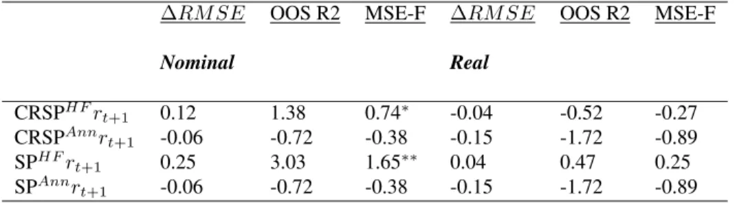
1.3 Out-Of-Sample Performance- 20 Years After the Sample

This table provides the out-of-sample results for both the mixed frequency and annual methods, denoted asHF andAnnrespectively. The dependent variables are returns, both nominal and real. All numbers reported are in percentage terms.

∆RM SE is the RMSE difference between the unconditional and conditional forecast for the same sample/forecast period. A positive number signifies superior OOS conditional forecast. The OOS statistics are calculated as reported in section

1.3.5. Significance levels are based off of the bootstrap procedure described in the section. . . . 22

1.4 Out-Of-Sample Performance- 1965-2017

This table provides the out-of-sample results for both the the mixed frequency and annual methods, denoted asHF andAnnrespectively. The dependent variables are returns, both nominal and real. All numbers reported are in percentage terms.

∆RM SE is the RMSE difference between the unconditional and conditional forecast for the same sample/forecast period. A positive number signifies superior OOS conditional forecast. The OOS statistics are calculated as reported in section

1.3.5. Significance levels are based off of the bootstrap procedure described in the section. . . . 23

1.5 Out-Of-Sample Performance- 20 Years After the Sample

This table provides the out-of-sample results for both the the mixed frequency and annual methods, denoted asHF andAnnrespectively. The dependent variables are nominal returns. All numbers reported are in percentage terms.∆RM SEis the RMSE difference between the unconditional and conditional forecast for the same sample/forecast period. A positive number signifies superior OOS conditional forecast. The OOS statistics are calculated as reported in section 1.3.5. Significance

(10)

1.6 Out-Of-Sample Performance- CRSP Data

This table provides the out-of-sample results for the mixed frequency estimation. The dependent variables are either returns or the equity premium, both nominal and real. Panel A reports results for equation (1.3.8) while Panel B reports results for equation (1.3.9). All numbers reported are in percentage terms.∆RM SEis the RMSE difference between the unconditional and conditional forecast for the same sample/forecast period. A positive number signifies superior OOS conditional forecast. The OOS statistics are calculated as reported in section 1.3.5. Significance

levels are based off of the (McCracken, 2007) asymptotic values. . . 25

1.7 Out-Of-Sample Performance- SP500 Data

This table provides the out-of-sample results for the mixed frequency estimation. The dependent variables are either returns or the equity premium, both nominal and real. Panel A reports results for equation (1.3.8) while Panel B reports results for equation (1.3.9). All numbers reported are in percentage terms.∆RM SEis the RMSE difference between the unconditional and conditional forecast for the same sample/forecast period. A positive number signifies superior OOS conditional forecast. The OOS statistics are calculated as reported in section 1.3.5. Significance

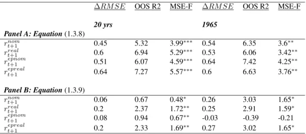
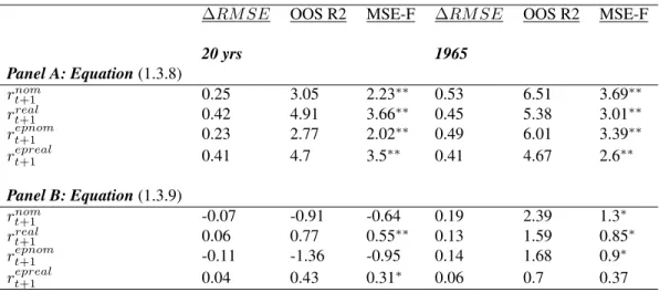
1.8 Out-Of-Sample Performance- Equation (1.3.11)

This table provides the out-of-sample results for the mixed frequency estimation. The dependent variables are either returns or the equity premium, both nominal and real. Panel A reports results for the CRSP data while Panel B reports results for the SP500 data. All numbers reported are in percentage terms. ∆RM SE is the RMSE difference between the unconditional and conditional forecast for the same sample/forecast period. A positive number signifies superior OOS conditional forecast. The OOS statistics are calculated as reported in section 1.3.5. Significance

1.9 Certainty Equivalent (CEV) Gains of SP500

This table provides the out-of-sample CEV gains in percent for the mixed frequency model (equation (1.3.3)) over the annual single frequency (equation (1.3.4)). Panel A reports results for the models with a single predictor. Panel B reports results

when controls are used as specified in equation (1.3.11) are reported as well. . . 29

1.10 Long Horizon Predictability- CRSP Dividend Growth and Returns

This table provides empirical results for long horizon predictability for both divi-dend growth and returns (nominal and real). Below,Kdenotes the horizon in years, Coef. is the estimated coefficient,ST is as defined in equation (1.4.6), andSRT is

as defined in equation (1.4.7). As usual, *, **, *** denote statistical significance at

the10%,5%, and1%levels, respectively. . . 33

1.11 Long Horizon Predictability- SP500 Dividend Growth and Returns

This table provides empirical results for long horizon predictability for both divi-dend growth and returns (nominal and real). Below,Kdenotes the horizon in years, Coef. is the estimated coefficient,ST is as defined in equation (1.4.6), andSRT is

as defined in equation (1.4.7). As usual, *, **, *** denote statistical significance at

(11)

1.12 Long Horizon Equity Premium Predictability

This table provides empirical results for long horizon equity premium (nominal and real) predictability for both CRSP and SP500. Below,Kdenotes the horizon in years, Coef. is the estimated coefficient,ST is as defined in equation (1.4.6),

andSRT is as defined in equation (1.4.7). As usual, *, **, *** denote statistical

significance at the10%,5%, and1%levels, respectively. . . 36

1.13 Out-Of-Sample Performance- Real Dividend Growth

This table provides the out-of-sample results for the mixed frequency estimation. The dependent variables are long horizon real dividend growth. All numbers reported are in percentage terms.∆RM SEis the RMSE difference between the unconditional and conditional forecast for the same sample/forecast period. A positive number signifies superior OOS conditional forecast. The OOS statistics are calculated as reported in section 1.3.5. Significance levels are based off of the

bootstrap procedure described in earlier sections. . . 38

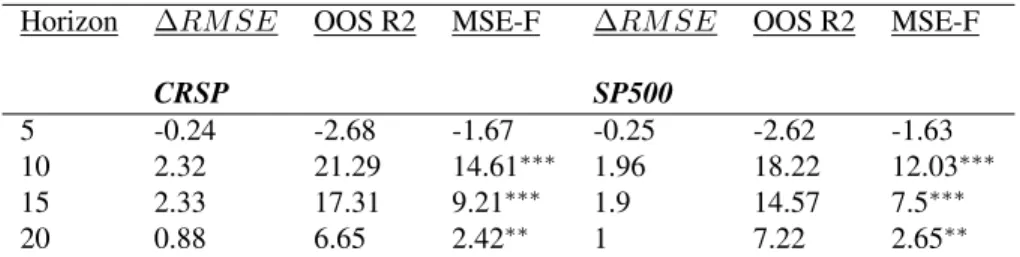
1.14 Out-Of-Sample Performance- Real Returns

This table provides the out-of-sample results for the mixed frequency estimation. The dependent variables are long horizon real returns. All numbers reported are in percentage terms.∆RM SEis the RMSE difference between the unconditional and conditional forecast for the same sample/forecast period. A positive number signifies superior OOS conditional forecast. The OOS statistics are calculated as reported in section 1.3.5. Significance levels are based off of the bootstrap

procedure described in earlier sections. . . 38

1.15 Out-Of-Sample Performance- Real Equity Premium

This table provides the out-of-sample results for the mixed frequency estimation. The dependent variables are long horizon real equity premiums. All numbers reported are in percentage terms.∆RM SEis the RMSE difference between the unconditional and conditional forecast for the same sample/forecast period. A positive number signifies superior OOS conditional forecast. The OOS statistics are calculated as reported in section 1.3.5. Significance levels are based off of the

1.16 Out-Of-Sample Performance- Nominal Equity Premium

This table provides the out-of-sample results for the mixed frequency estimation. The dependent variables are long horizon nominal equity premiums. All numbers reported are in percentage terms.∆RM SEis the RMSE difference between the unconditional and conditional forecast for the same sample/forecast period. A positive number signifies superior OOS conditional forecast. The OOS statistics are calculated as reported in section 1.3.5. Significance levels are based off of the

2.1 Descriptive statistics

The reported statistics include the mean, the minimum (Min) and maximum (Max), standard deviation (SD), Skewness (Skew.), Kurtosis (Kurt.), and the number of

(12)

2.2 Contemporaneous correlations between monthly realized volatilities.

The table reports the contemporaneous correlations between the various realized

volatilities. The sample covers the 2013M05 - 2017M12 period. . . 49

2.3 Bitcoin: financial and macroeconomic explanatory variables.

The table reports estimation results for the GARCH-MIDAS-X models including 3 MIDAS lag years (K = 36) of a monthly explanatory variableX. The sample period is 2013M05 - 2017M12. The conditional variance of the GARCH(1,1) is specified ashi,t =m+αε2i−1,t+βhi−1,t. The numbers in parentheses are HAC

standard errors.???,??,?indicate significance at the 1%, 5%, and 10% level. LLF is the value of the maximized log-likelihood function. AIC and BIC are the Akaike

and Bayesian information criteria. . . 51

2.4 S&P 500

2.5 Nikkei 225

2.6 Gold and Copper

The table reports estimation results for the GARCH-MIDAS-X models including 3 MIDAS lag years (K = 36) of a monthly explanatory variableX. The sample period is 2013M05 - 2017M12. The conditional variance of the GARCH(1,1) is specified ashi,t =m+αε2_i−1,t+βhi−1,t. The numbers in parentheses are HAC

2.7 Bitcoin specific explanatory variables

(13)

3.1 NFP (As Reported, Revised), Estimize, and Consensus

Sample statistics for the As Reported and Revised NFP data, as well as for the forecasts from Estimize and Consensus, as proxied by the survey of professional forecasts conducted by Bloomberg.

The sample is from May 2014 - February 2017. The column labeleved pval contailes the p-value of a two-tailed t-test of equality of means between the Estimize and Consensus values in each row. The *,**,*** denote statistical significance at the10%,5% 1%levels, respectively. Data is in thousands (’000). Each entry is an ensemble average summarizing first over forecasts in a given month, and then

across the months. . . 64

3.2 Definitions of forecasting accuracy and bias whereF denotes the forecast of the NFP value, andAdenotes the actual NFP value. Subscriptsicapture individual

forecasts, andtindicates the calendar month of the NFP event. . . 65

3.3 Sample Statistics for As Reported and Revised NFP Data

Sample statistics for each of the accuracy and bias measures outlined in Table 2 for both the Estimize and Consensus forecasts. The top panel bases the computations off of As Reported NFP data, and the bottom panel bases the computations off of Revised NFP data. The statistics reported are the averages of monthly values. The columnnreports the average number of participants throughout our sample, and pval reports the p-value for a two-tailed t-test of the equality of means. The *, **, *** denote statistical significance at the10%,5%, and1%levels, respectively. The

sample is from May 2014 - February 2017. . . 67

3.4 Accuracy of the “All Stars” Forecasters for As Reported and Revised NFP Data The top 10 rows are results using As Reported NFP data and the bottom 10 rows are results using Revised NFP data. Rank is determined by calculating individual forecaster’sAF Eover time and then rank ordering from lowestAF Eto highest. Only those who had at least two forecasts over the entire sample were considered.

AF EC is theAF E as defined in Table 2 for Consensus andAF EE is defined analogously for Estimize. “Diff.” is the differenceAF EC −AP EE, andpval

reports the p-value for the test of the equality of means. The, *, **, *** denote statistical significance at the10%,5%, and1%levels, respectively. The sample is

from May 2014 - February 2017. . . 69

3.5 “Regular” Forecasters for As Reported and Revised NFP Data

Forecasting accuracy within four bins: those who participate less than25%of the time, those who participate between25−49%of the time, those who participate between50−74%of the time, and those who participate at least75%of the time.

AF Eis as defined in Table 2, andN is the number of forecasters. The superscripts “C” and “E” denote Consensus and Estimize respectively. “Diff.” is the difference

AF EC−AF EE, andpvalreports the p-value for the test of the equality of means. The top panel presents results for the As Reported data while the bottom panel presents results for the Revised data. The *, **, *** denote statistical significance at the10%,5%, and1%levels, respectively. The sample used is from May 2014

(14)

3.6 Forecasting Horizon for As Reported and Revised NFP Data

Horizon is defined as the difference between the date of a particular month’s NFP forecast and the date of the associated NFP release. The horizon is grouped into buckets: 1 week prior to release, 2 weeks prior to release, 3 weeks prior to release, 4 weeks prior to release and over 4 weeks prior to the NFP release. AF E is as defined in Table 2 andN is the number of forecasters. The superscripts “C” and “E” denote Consensus and Estimize, respectively. “Diff.” is the difference

AF EC−AF EE, andpvalreports the p-value for the test of the equality of means. The top panel presents results for As Reported NFP data while the bottom panel presents results for Revised data. The *, **, *** denote statistical significance at

the10%,5%, and1%levels, respectively. The sample is from May 2014 - February 2017. . . . 71

3.7 Boldness for As Reported and Revised NFP Data

The top 3 rows are results using As Reported NFP data and the bottom 3 rows

are results using Revised NFP data. Boldness is computed as |F pop i,t −F

f ull t |

Fpopt

for every individual forecast,i, from the Consensus and Estimize sample and grouped into bins: low, medium and high boldness. AF Eas defined in Table 2, andN is the number of forecasters. The superscripts “C” and “E” denote Consensus and Estimize, respectively. “Diff.” is the differenceAF EC−AF EE, andpvalreports the p-value for the test of the equality of means. The *, **, *** denote statistical significance at the10%,5%, and1%levels, respectively. The sample is from May

2014 - February 2017. . . 73

3.8 Uncertainty&Diversity for As Reported and Revised NFP Data

The top 3 rows are results using As Reported NFP data and the bottom 3 rows are results using Revised NFP data.V andρare calculated as per equations 3.4.1 and 3.4.2, and grouped into low, medium, and high. “Diff.” is the difference

AF EC −AF EE, and pval reports the p-value for the test of the equality of means. The *, **, *** denote statistical significance at the 10%, 5%, and 1%

levels, respectively. The sample is from May 2014 - February 2017. . . 75

3.9 Multivariate Regression for As Reported NFP Data

Results for Equation 3.4.3 estimated via OLS on As Reported data. The column “Estimate” reports the estimated coefficient for each variable. HorC −HorE

is the difference in horizon, where horizon is defined as in 3.4.2 subsection, for Consensus and Estimize. NC₋_NE _{is the difference in the number of forecasters}

for Consensus and Estimize. ρC −ρE andVC −VE are defined as subsection 3.4.4.BestC%−BestE%is the difference in the percentage of top forecasters in each month for Consensus and Estimize.RegC%−RegE%is the difference in the percentage of regular forecasters in each month for Consensus and Estimize. SE reports the standard error of each estimated coefficient. t-stat reports the calculated t-statistic for each estimate and pval reports the p-value for the corresponding t-statistic. The, *, **, *** denote statistical significance at the10%,5%, and1%

(15)

3.10 Multivariate Regression for Revised NFP Data

Results for Equation 3.4.3 estimated via OLS on Revised data. The column “Estimate” reports the estimated coefficient for each variable. HorC −HorE

is the difference in horizon, where horizon is defined as in 3.4.2 subsection, for Consensus and Estimize. NC−NE is the difference in the number of forecasters for Consensus and Estimize. ρC −ρE andVC −VE are defined as subsection 3.4.4.BestC%−BestE%is the difference in the percentage of top forecasters in each month for Consensus and Estimize.RegC%−RegE%is the difference in the percentage of regular forecasters in each month for Consensus and Estimize. SE reports the standard error of each estimated coefficient. t-stat reports the calculated t-statistic for each estimate and pval reports the p-value for the corresponding t-statistic. The, *, **, *** denote statistical significance at the10%,5%, and1%

levels, respectively. The sample is from May 2014 - February 2017. . . 77

3.11 “Regulars” Multivariate Regression for As Reported NFP Data

Results for Equation 3.4.4 estimated via Panel OLS for As Reported data. All regressors are constructed at the individual forecaster level.HorC−HorE is the difference in forecasting horizon,boldC−boldE is the difference in the measure of boldness, whileρC−ρE andVC −VE are as defined in subsections 3.4.2 and 3.4.4. t-stat reports the calculated t-statistic for each estimate, andpval reports the p-value for the corresponding t-statistic. The *, **, *** denote statistical significance at the10%,5%, and1%levels, respectively. The sample is from May

2014 - February 2017. . . 78

3.12 “Regulars” Multivariate Regression for Revised NFP Data

Results for Equation 3.4.4 estimated via Panel OLS for Revised data. All regressors are constructed at the individual forecaster level. HorC −HorE is the difference in forecasting horizon,boldC−boldE is the difference in the measure of boldness, whileρC₋_ρE_and_VC ₋_VE _{are as defined in subsections 3.4.2 and 3.4.4. t-stat}

reports the calculated t-statistic for each estimate, andpvalreports the p-value for the corresponding t-statistic. The, *, **, *** denote statistical significance at the

10%,5%, and1%levels, respectively. The sample is from May 2014 - February 2017. . . 79

3.13 “All Stars” Multivariate Regression for As Reported NFP Data

OLS regression output for As Reported NFP data using only the best forecasters. All regressors are also constructed at the individual forecaster level.HorC−HorE

is the difference in forecasting horizon, boldC −boldE is the difference in the measure of boldness, whileρC−ρEandVC −VE are as defined in subsections 3.4.2 and 3.4.4. t-stat reports the calculated t-statistic for each estimate andpval

reports the p-value for the corresponding t-statistic. The *, **, *** denote statistical significance at the10%,5%, and1%levels, respectively. The sample is from May

(16)

3.14 “All Stars” Multivariate Regression for Revised NFP Data

OLS regression output for As Reported NFP data using only the best forecasters. All regressors are also constructed at the individual forecaster level.HorC−HorE

is the difference in forecasting horizon, boldC −boldE is the difference in the measure of boldness, whileρC−ρEandVC −VE are as defined in subsections 3.4.2 and 3.4.4. t-stat reports the calculated t-statistic for each estimate andpval

reports the p-value for the corresponding t-statistic. The *, **, *** denote statistical significance at the10%,5%, and1%levels, respectively. The sample is from May

2014 - February 2017. . . 80

B.1 Flight-to-safety

B.2 USD - Korean Won

B.3 USD - JPY

B.4 CNY - USD

(17)

LIST OF FIGURES

1.1 CRSP and SP500 Dividend Price Ratio

This figure depicts the annually constructed dividend price ratio for CRSP and the SP500. . . . 10

1.2 CRSP and SP500 Dividend Price Ratio Weighting Schemes

This figure depicts the MIDAS regressions Almon weighting schemes for equation (1.3.1). . . 12

1.3 CRSP and SP500 Dividend Price Ratio Weighting Schemes

This figure depicts the MIDAS regressions Almon weighting schemes for equation (1.3.2). . . 12

1.4 CRSP and SP500 Dividend Price Ratios

This figure depicts the mixed frequency constructed dividend price ratio for CRSP

and the SP500, both returns and dividend growth weighting schemes. . . 13

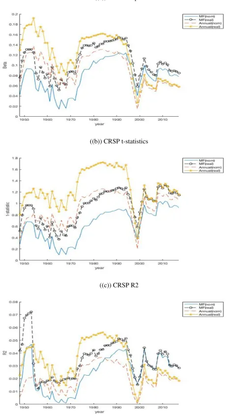
1.5 Expanding Window Returns Regressions (CRSP Data)

This figure plots the expanding window estimated return coefficients, their respec-tive t-statistics and R2 for the mixed frequencydptand the annualdpt. Each is

estimated with real and nominal returns. The sample is 1928 to 2017. . . 16

1.6 Expanding Window Dividend Growth Regressions (CRSP Data)

This figure plots the expanding window estimated dividend growth coefficients, their respective t-statistics and R2 for the mixed frequencydptand the annualdpt.

Each is estimated with real and nominal dividend growth. The sample is 1928 to 2017. . . 17

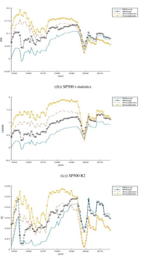
1.7 Expanding Window Returns Regressions (SP500 Data)

This figure plots the expanding window estimated return coefficients, their respec-tive t-statistics and R2 for the mixed frequencydptand the annualdpt. Each is

estimated with real and nominal returns. The sample is 1928 to 2017. . . 19

1.8 Expanding Window Dividend Growth Regressions (SP500 Data)

This figure plots the expanding window estimated dividend growth coefficients, their respective t-statistics and R2 for the mixed frequencydptand the annualdpt.

Each is estimated with real and nominal dividend growth. The sample is 1928 to 2017. . . 20

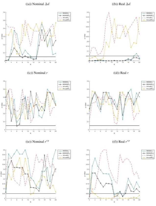
1.9 Long HorizonST andSRT p-values

This figure plots the p-values of the long horizon predictive coefficients for both CRSP and the SP500 for the signed test and signed rank test. Each plot has the p-values using real and nominal returns/dividend growth/ equity premium. The

sample is 1928 to 2017.. . . 34

1.10 CRSP Long HorizonST andSRT p-values

This figure plots the p-values of the long horizon predictive coefficients for the signed test and signed rank test. In each plot, the mixed frequency (MIDAS) results are plotted with the annual single frequency results. Each plot has the p-values using real and nominal returns/dividend growth/ equity premium. The sample is

(18)

2.1 Bitcoin Price development in the 2013:M5 to 2017:M12 period . . . 47

2.2 Annualized monthly realized volatilities . . . 49

2.3 Baltic Dry Index and RV Glux

The figure shows the annualized long-term (bold red line) and short-term (black line) volatility components as estimated by the GARCH-MIDAS models with the Baltic dry index (left) and the realized volatility of the luxury goods index (right)

as explanatory variables. . . 52

3.1 Monthly Participants for Estimize and Consensus

Numbers of participants making NFP forecasts in each month from April 2014 -February 2017. The number of Estimize forecasters is indicated in red, and the

number of Consensus forecasters, as measured by Bloomberg, is indicated in blue. . . 63

3.2 Estimize and Consensus Monthly Forecasts

Box plots of individual NFP forecasts for each month of the sample (May 2014 -February 2017). The top panel captures forecasts from Estimize, while the bottom

panel captures forecasts from Consensus, as measured by Bloomberg. . . 65

3.3 Monthly average AFE of Estimize and Consensus for NFP Data

Monthly averageAF E(as defined in Table 3.2) for Consensus forecasts (in black) and Estimize forecasts (in red) during the period May 2014- February 2017. The left hand panel computes the AFE relative to the As Reported NFP data, while the

right hand panel computes the AFE relative to the Revised NFP data. . . 66

A.1 Expanding Window Dividend Growth Regressions (CRSP Data)

This figure plots the expanding window estimated p-value for the Wald Test. I test the null hypothesis that all 12 estimated monthly weights are equal to zero. The

dependant variable is real and nominal dividend growth. The sample is 1928 to 2017. . . 82

A.2 Expanding Window Dividend Growth Regressions (SP500 Data)

dependant variable is real and nominal dividend growth. The sample is 1928 to 2017. . . 82

A.3 Expanding Window Returns Regressions (CRSP Data)

dependant variable is real and nominal returns. The sample is 1928 to 2017.. . . 83

A.4 Expanding Window Returns Regressions (SP500 Data)

(19)

A.5 Russell 2000 Index Out-of-Sample Performance

This figure depicts the (Welch and Goyal, 2007) annual OOS performance for both returns and the dividend growth ratio. As per (Welch and Goyal, 2007), the y-axis is the cumulative squared prediction errors of the null model minus the cumulative squared prediction error of the alternative model. An increase in the lines indicates better performance of the mixed frequency model, while a decrease

in a line indicates better performance of the null. . . 84

A.6 Canada SP/TSX Composite Index Out-of-Sample Performance

A.7 FTSE All Shares Index Out-of-Sample Performance

A.8 FTSE Euro First 300 Index Out-of-Sample Performance

A.9 CRSP Index Out-of-Sample Performance equation 1.3.8

This figure depicts the (Welch and Goyal, 2007) annual OOS performance for both real and nominal equity premium. As per (Welch and Goyal, 2007), the y-axis is the cumulative squared prediction errors of the null model minus the cumulative squared prediction error of the alternative model. An increase in the lines indicates better performance of the mixed frequency model, while a decrease

(20)

A.11 SP500 Index Out-of-Sample Performance equation 1.3.8

(21)

CHAPTER 1

A Mixed Frequency Approach to Return and Dividend Growth Predictability

1.1 Introduction

The return predictability literature has accumulated a large body of evidence documenting both the existence

and lack thereof of market return predictability. Despite the contradictory findings, the general impression

is that market returns are predictable (see Lettau and Ludvigson (2001) and Welch and Goyal (2007)) by

a number of financial variables, you just have to find the right combination of variables. This paper poses

the question: what if it is not just about the right combination of variables, but also the choice of sampling

frequencyin estimation?

One branch of the literature is mainly concerned with finding possible predictors while another analyzes

return predictability in conjunction with dividend growth predictability. This paper considers the latter and

provides a comprehensive study, examining the in-sample and out-of-sample predictability of market returns

and dividend growth through the application of the mixed frequency data sampling (MIDAS regressions)

approach of Ghysels et al. (2006). I examine formally whether systematic differences exist in the predictive

ability of the mixed frequency regression approach and the single frequency approach commonly used in

the literature for both dividend growth and market returns. Then, I consider the performance of the mixed

frequency approach with the inclusion of control variables and at longer horizons.

The time series models used in the literature generally involve data sampled at the same frequency.

However, some models might predict long-term market returns better than short-term returns, or vice-versa.

Given this, it is not uncommon to look at multiple frequencies when exploring return predictability (see

Welch and Goyal (2007), Ang (2011), Engsted and Pedersen (2009), Chen (2009), and others).

By only estimating models involving data sampled at the same frequency, we are not fully exploiting all

(22)

which is the most common one used within the literature:

rt+1=β0+β1xt+t+1 (1.1.1)

wherer is market return andxis some predictor. In this case, we are only using some annual aggregate

predictor. Though, this predictor may be available at a much higher frequency, say monthly. By estimating

equation (1.1.1) at the annual aggregate frequency, we are implicitly forcing each month to have the same

effect on returns. If this assumption does not hold true then the model might potentially be misspecificied

and potentially useful information may be destroyed.

Recently, econometric models that take into account information in unbalanced frequencies have attracted

substantial attention. In particular, the application of the MIDAS regression approach has amassed a

substantial literature. It is particularly attractive given that it exploits a much larger information set and is

more flexible than say equation (1.1.1). Many studies have uncovered relationships between the data that was

previously undetectable due to data aggregation. For example, Ghysels et al. (2005) used MIDAS volatility

models and uncovered a significantly positive relation between risk and return. Clements and Galv˜ao (2008)

find that MIDAS regressions can lead to improvements in forecasting current and next quarter output growth.

For the sake of brevity I omit many other examples from the literature.1

This paper explores whether or not relationships between the data was possibly undetectable due to

data aggregation. Specifically, MIDAS regression weights are only applied to the monthly dividends in the

dividend price ratio, the main predictor under consideration here. I allow dividends paid out in different

months to be weighted differently and keep the end of year price constant when constructing the annual

mixed frequency dividend price ratio. In many cases I uncover predictability (for dividend growth, market

returns and the equity premium) and this finding is robust to horizon. This paper shows that we can uncover

dividend growth predictability and that we can improve out-of-sample return predictability by leveraging

higher frequency data.

Furthermore, I uncover statistically significant long horizon predictability for dividend growth for

domestic aggregate equity markets. Here, I am able to estimate all coefficients with the theoretically correct

sign and uncover statistical significance at long horizons for the both the SP500 and CRSP. In this paper,

1

(23)

I also show that using MIDAS regressions can result in superior out-of-sample return predictability when

compared to the conventional annual frequency.

The findings of this paper have implications for both the return predictability literature and for other

applications in finance, such as portfolio management. Most applications of portfolio management require a

robust method out-of-sample to forecast expected market returns. The mixed frequency dividend price ratio

predictor proposed here meets much of that criteria, especially when combined with other predictors. There

are important implications for the asset pricing literature in general here as well, especially in applications

where the dividend price ratio is assumed to be a satisfactory proxy for expected stock returns.

1.1.1 Motivation and Related Literature

The present value decomposition from Campbell and Shiller (1988) suggests that the dividend price ratio

must be related to either future returns or future dividend growth. It is possible for both future returns and

future dividend growth to be predictable by the dividend price ratio, but at least one must be significantly

related to it. Put differently, any variation in the dividend price ratio must be caused by either movement in

expected returns, dividend growth, or both.

If the dividend price ratio were constant, then neither expected returns nor dividend growth would be

forecastable by it. We know that the dividend price ratio is not constant over time: it does move. The

present value identity then implies that at least one of either expected returns or dividend growth should be

forecastable by the dividend price ratio. This relation is why the dividend price ratio is almost always chosen

as a possible predictor of returns or dividend growth while other market ratios have assumed a secondary role.

Most of the research within the literature centers around return predictability, as the most common

finding is that dividend price ratio is only significantly related to returns (see Lettau and Ludvigson (2005)

Cochrane (2007), Lettau and Van Nieuwerburgh (2007), among others). Some studies found that small

adjustments to the classic dividend price ratio can even improve the relation with market returns. Lacerda

and Santa-Clara (2010) are able to improve forecasts of both returns and dividend growth by incorporating

the moving averages of past dividend growth into the dividend price ratio. Lettau and Nieuwerburgh (2008)

adjust the dividend price ratio to accommodate for shifts in the steady state of the economy and find strong

evidence of in-sample return predictability.

A few studies that looked at international equity markets have uncovered a significant relationship

(24)

(2014). Maio and Santa-Clara (2015) find that there is strong evidence of dividend growth predictability by

the dividend price ratio when one looks at the cross-section of stock returns. Kelly and Pruitt (2013) showed

that by using cross-sectional firm disaggregated data one can successfully uncover a significant relationship

between the dividend price ratio and dividend growth. Chen (2009) finds that the lack of detection of a

significant relationship between dividend growth and the dividend price ratio for aggregate markets is in part

due to postwar dividend smoothing by firms.

Recently, Asimakopoulos et al. (2017) use MIDAS regressions and regress monthly dividend price ratio

growth data on annual dividend growth data. They decompose the dividend price ratio into two components:

dividend price ratio growth, which is the high frequency component, and lagged annual dividend price ratio.

Their findings suggest that it is the dividend price ratio growth that is the predictable component of the

dividend price ratio.

This paper builds upon their findings and shows that it is not just the dividend price ratio growth that

is the predicable component. Specifically, here MIDAS regression weights are only applied to the monthly

dividends in the dividend price ratio, as opposed to dividend price ratio growth as in Asimakopoulos et al.

(2017). Asimakopoulos et al. (2017) only consider the relationship between the dividend price ratio and

dividend growth. While I consider dividend growth, I also examine the relationship between the dividend

price ratio and returns. To the best of my knowledge, this is the first paper to apply a mixed frequency

approach to examine the relationship between the dividend price ratio and returns.

The general consensus within the literature continues to be that the dividend price ratio is mainly related

to expected returns for aggregate equity markets, especially at longer horizons. The empirical findings for

US equity markets within the literature are counter intuitive to the classic asset pricing theories2. With the

application of MIDAS regressions, I show that this is not the case.

This finding that the dividend price ratio is strongly related to market returns can be heavily impacted

by the data. Ang (2011), Ang and Bekaert (2006) and Goyal and Welch (2003) find that returns are not

predictable by the dividend price ratio when the 1990’s are included in the estimation period. Chen (2009)

concluded that returns are strongly related to the dividend price ratio, but mainly in the post war period

(1946-2005). This finding of predictability is also rarely validated out-of-sample, aside from that of Chen

(2009), Welch and Goyal (2007), Lacerda and Santa-Clara (2010) and Goyal and Welch (2003). In this

2

(25)

paper, I show that using MIDAS regressions can result in superior out-of-sample return predictability when

compared to the conventional annual frequency.

The paper is organized as follows: section 1.2 describes the data and methodology used in the analysis. It

will also provide a brief description of MIDAS regressions and the Almon polynomial. Section 1.3 presents

empirical findings at the annual horizon. Section 1.4 presents empirical findings at long horizons. Finally,

section 1.5 concludes the paper.

1.2 Data and Methodology

In this section, I discuss the Campbell and Shiller (1988) present value identity in more detail. Then I present

a more in formal overview of the econometric methodology utilized within this paper. Finally, this section

will detail the source and construction of the data used in empirical estimation.

1.2.1 The Present Value Model

To derive the present value model we first start with the definition of returns, where asset returns are comprised

of capital gains yield and dividend yield. Specifically, we write returns asRt+1 = Pt+1+_P_tDt+1, whereP

denotes the price and D denotes dividends. Let rt = log(1 +Rt), pt = log(Pt), dt = log(Dt), and

dpt=logD_P_tt. Taking a first-order Taylor approximation yields the original Campbell and Shiller (1988) log

linearized model.

dpt≈ −κ+rt+1−∆dt+1+ρ(dpt+1)

Whereρ≡exp(p−d)/1 + exp(p−d) = (P /D)/(1−(P /D))∈(0,1)is the log linearization discount

coefficient andκ=−ln(1−ρ)−ρln((1/1−ρ)−1)is defined as a constant.

Following Cochrane (2007) and iterating the Campbell and Shiller (1988) equationktimes,

dpt≈

−κ(1−ρk) 1−ρ +

k

X

j=1

ρj−1rt+j− k

X

j=1

ρj−1∆dt+j +ρk(dpt+k) (1.2.1)

gives us the present-value relation, which says that the current log dividend price ratio is positively related

with future discounted log returns and future discounted log dividend price ratio at timet+k. From the

relation, the log dividend price ratio is negatively related with future discounted log dividend growth. This

(26)

assume no bubbles the present value decomposition states that the dividend price is equal to a constant plus

the difference between the future discounted returns and the future discounted dividend growth.

Methods commonly used in the literature to estimate the model are long horizon regressions and VAR’s.

One convention is to follow Cochrane (2007) and to directly estimate weighted long-horizon regressions of

future log returns, log dividend growth and log dividend to price ratio on the current dividend to price ratio.

The second method is to run a first-order VAR as in Cochrane (2007), Engsted and Pedersen (2009), Maio

and Santa-Clara (2015), and others.

1.2.2 The Almon Polynomial and MIDAS Regressions

First I briefly discuss the Almon polynomial and distributed lag models, then I move onto MIDAS regressions.

If we have reason to believe that our dependant variable,yt, is affected by more than one lag of our explanatory

variables,x_t−(M−1), ..., xt−1, xt, we can write a distributed lag model in the following form:

yt= K−1

X

k=0

wkxt−k+t (1.2.2)

whereK is equal to the lag length.

The Almon polynomial distributed lag structure was put forth by Almon (1965) and has since become

one of the most popular lag structures implemented in distributed lag models. The polynomial is defined as

follows:

wk= p

X

j=0

θjij (1.2.3)

wherek= 0,1,2, ...., K−1andpis the degree of the polynomial. Given that the order of the polynomial

is much lower than that of the lag length,K, the resulting Almon distributed lag model can be estimated

parsimoniously via OLS.

Define a MIDAS regression model as follows with a basic single high frequency regressor (one-step

ahead).

yL_t₊₁ =β0+β1 K−1

X

k=0

(27)

The MIDAS regression weights are governed by polynomial specifications.3 The weighting scheme is purely

data driven, there are no assumptions required for estimation and MIDAS does not suffer from parameter

proliferation.

Combining equation (1.2.2) with (1.2.3) is a specific case of MIDAS regressions, which can be estimated

via OLS. Throughout this paper, I will use the Almon polynomial for estimation with degree set to two. A

quadratic Almon polynomial is able to take on many shapes, they can be very similar to the Beta weighting

function and the Exponential Almon weighting function. Estimating via OLS will allow us to stay very

close to the Campbell and Shiller (1988) framework and utilize evaluation methods which will ease any

comparisons within the literature.

The Almon polynomial, as specified above, does not necessarily result in MIDAS regression weights that

sum to one. The estimation of Almon lags in MIDAS regressions via OLS requires properly transformed

high frequency data regressors. Once the weights are estimated, given that they do not sum to zero, they

can be re-scaled to obtain the slope coefficients and normalized weights. I recover the slope coefficient and

normalize the weights so that they do sum to one throughout this paper. Hence, the equations specified in the

following sections will be written under this assumption.4

Normalizing the weights after estimation ensures that the weights sum to one, then our high-frequency

slope, β1, is identified. This process is what weights each monthly observation (dividends) differently.

Motivated by the findings of Asimakopoulos et al. (2017), I focus on monthly data rather than quarterly.

Asimakopoulos et al. (2017) demonstrated that even aggregating at the quarterly frequency resulted in a loss

of useful information.

All of the empirical analysis that follows was also estimated via MIDAS profiling (put forth by Ghysels

and Qian (2019)) with the exponential Almon and Beta weighting schemes. The results and conclusions

are largely the same. I choose to report results estimated with the Almon polynomial MIDAS regressions

technique rather than the MIDAS profiling method so as to avoid any possible generated regressor issues.

3

For a more detailed treatment of MIDAS weighting schemes see Ghysels et al. (2007)

4

(28)

1.2.3 Data

The bulk of this analysis is concerned with domestic equity market data. The main domestic data are from

the CRSP value-weighted portfolio and from the SP500 value-weighted portfolio. Both domestic data sets

span from January 1927 to December 2017. These are the two most commonly used data sets within the

literature, see Cochrane (2007), Maio and Santa-Clara (2015), Engsted and Pedersen (2009), Campbell and

Shiller (1988), and others. The CRSP data is a total market measures, it consists of all firms listed on US

stock exchanges. CRSP consists of small, medium, and large cap stocks while SP500 only has large caps. I

also consider the Russell 2000 Index obtained from Factset. The data set spans from 1980 to 2018.

Some of the analysis will consider international equity market data. I follow Asimakopoulos et al.

(2017) and Engsted and Pedersen (2009) who look at international equity markets alongside domestic. The

international data are from Factset and consist of three different large equity market indices. I consider the

FTSE All Shares Index, the FTSE Euro First 300 Index, and the Canada SP/TSX Composite Index. All of the

international data sets span from 1987 to 2018.

Within the literature, there are two common ways of constructing the dividend price ratio. Cochrane

(2007), Maio and Santa-Clara (2015) and many others do assume that monthly dividends are reinvested in the

stock market. Under reinvestment, the dividend price ratio is constructed from the difference between the

value-weighted returns with dividends and the value-weighted returns excluding dividends.5

Campbell and Shiller (1988), Chen (2009), Ang (2011), Ang and Bekaert (2006) and others construct

the dividend price ratio assuming that monthly dividends are not reinvested in the stock market. Under this

assumption, monthly dividends are recovered from the weighted returns with dividends and the

value-weighted returns excluding dividends. The monthly dividends are then summed to get annual dividends.6

Here, I assume no reinvestment and apply MIDAS regression weights to only the monthly dividends.

5

See Cochrane (2007) for an in depth explanation of calculations.

6

(29)

1.3 Annual Empirical Results

1.3.1 One Year Ahead Predictability

In this section, the empirical results for equity markets are presented. All empirical results that follow in this

section are for one step ahead (annual) horizons. Before we look at the empirical results of the models we

will first briefly look at the data.

1.3.2 Properties of the data

Table 1.1 displays the annual sample statistics for both the annual dividend growth rate and the returns. I

report the annual mean, maximum, minimum, standard deviation and auto-correlation(φ). There are no

issues of persistence with either dividend growth or returns. We can also see that the sample statistics for

both CRSP and the SP500 are very similar.

Figure 1.1 plots the annually constructed dividend price ratios7for both CRSP and the SP500. We see

that they track one another rather closely. Maio and Santa-Clara (2015) demonstrated that there are in fact

differences between what drives small cap vs. large cap stocks. CRSP consists of small, medium, and large

cap stocks while the SP500 is only tilted towards large cap stocks. As such, I expect to see differences in the

monthly weights.

Table 1.1: Sample Statistics for Annual Dividend Growth and Returns

This table provides sample mean, max, min, standard deviation and auto-correlation (φ) for the annual dividend growth, annual return and annual dividend price ratio. Panel A is for the CRSP data set. Panel B is for the SP500 data set.

Mean Max Min Std. φ

Panel A: CRSP Data

∆dL 0.05 0.43 -0.51 0.12 0.28

rL 0.09 0.45 -0.56 0.19 0.04

dpL -3.41 -2.35 -4.48 0.45 0.89

Panel B: SP500 Data

∆dL _0.05 _0.45 _-0.63 _0.13 _0.21

rL _0.09 _0.42 _-0.58 _0.19 _0.05

dpL _-3.38 _-2.29 _-4.45 _0.46 _0.88

7

(30)

Figure 1.1: CRSP and SP500 Dividend Price Ratio

This figure depicts the annually constructed dividend price ratio for CRSP and the SP500.

1.3.3 The Benefits of High Frequency Data

Within this subsection I explore the potential gains from utilizing high-frequency data by looking at large

equity market data. I only allow the monthly dividends to be weighted differently in the construction of

the dividend price ratio. In contrast, Asimakopoulos et al. (2017) allowed the monthly dividend price ratio

growth rate to be weighted differently. To test the possibility that dividends paid in certain months matter

more than other months of the year, we will first explore annual one year ahead regressions for large equity

markets. I then compare the results using the mixed frequency constructed dividend price ratio to that of the

conventional annually constructed dividend price ratio.

Table 1.2 presents the empirical results of the one year ahead regressions for both the CRSP and SP500

data sets. The following models are estimated,

∆dL_t₊₁=β0+β1dpLt(ω) +dt+1 (1.3.1)

rL_t₊₁ =β0+β1dpLt(ω) +rt+1 (1.3.2)

where, dpL_t(ω) = (

P12 j=1ωjdHj,t)

p12,t is the MIDAS regression weighted high frequency data. The model

(31)

MIDAS regressions via OLS requires properly transformed high frequency data regressors. Once the weights

are estimated via OLS, I rescale them to obtain the slope coefficient and normalized weights.

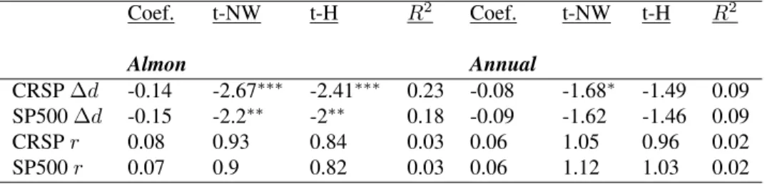
Table 1.2: Annual Regressions

This table provides empirical results for one-year ahead predictability. The dependent variables are the annual log dividend growth and annual log returns. The models are estimated via OLS. The resulting weights are normalized and the slope coefficient is recovered. T-NW reports the calculated Newey-West t-statistic for each estimate with one lag. T-H reports the calculated Hodrick (1992) 1B t-statistic for each estimate with one lag. As usual, *, **, *** denote statistical significance at the10%,5%, and1%levels, respectively.

Coef. t-NW t-H R2 _Coef. _t-NW _t-H _R2

Almon Annual

CRSP∆d -0.14 -2.67∗∗∗ -2.41∗∗∗ 0.23 -0.08 -1.68∗ -1.49 0.09 SP500∆d -0.15 -2.2∗∗ -2∗∗ 0.18 -0.09 -1.62 -1.46 0.09 CRSPr 0.08 0.93 0.84 0.03 0.06 1.05 0.96 0.02 SP500r 0.07 0.9 0.82 0.03 0.06 1.12 1.03 0.02

We can see from Table 1.2 that there are benefits to using high frequency data. Conventional estimation

involves equal weights, which implicitly forces each month to be as important as the rest. For the annual

CRSP data, there is only a statistically significant relationship with dividend growth at the 10% level, when

looking at the Newey and West (1987) t-statistics. When estimating with high frequency data, there is now

a statistically significant relationship with dividend growth at the 1% level, judged by both the Newey and

West (1987) t-statistic and the Hodrick (1992) t-statistic. For the SP500, we only see a statistically significant

relationship between the dividend price ratio and dividend growth when we estimate with Almon weights.

Given that neither the annual, nor mixed frequency approach resulted in a statistically significant

relationship between the dividend price ratio and returns, it is difficult to draw any conclusions in-sample.

However, it is important to note that there does exist a statistically significant relationship between returns

and the mixed frequency regressor if we consider different sampling periods.8

We can note that the mixed frequency approach resulted in slightly larger estimated coefficients andR2.9

From Table 1.2 we can see that this result of the mixed frequency approach having slightly larger estimated

coefficients holds true when either dividend growth or returns are the dependent variables. In regards to the

R2coefficients for dividend growth, the mixed frequency approach resulted in anR2that is almost150%

8

When the same mixed frequency model is estimated with the data spanning from 1950-2017, I find it is statistically highly significant. I also find it to be statistically highly significant when I only include the past 30 years of data.

9_{Note, this result holds for the different sampling periods as well. The mixed frequency model results in slightly larger coefficients}

andR2

(32)

larger than that of the annual approach. This is true for both CRSP and SP500 data. For returns, we see a

more modest increase in theR2of50%for both data sets.

For robustness, I also conduct an F-test test. The estimated mixed frequency coefficients are a linear

combination of the estimated monthly weights. The null hypothesis is that all weights are jointly equal to

zero. The resulting p-values when the dependant variable is returns, coincides with the results of Table 1.2

for both CRSP and SP500 data. For dividend growth, the CRSP data has statistical significance at well below

the 5% level. For the SP500 however, the resulting p-value from the F-test is 15%.

Figure 1.2: CRSP and SP500 Dividend Price Ratio Weighting Schemes

This figure depicts the MIDAS regressions Almon weighting schemes for equation (1.3.1).

Figure 1.3: CRSP and SP500 Dividend Price Ratio Weighting Schemes

This figure depicts the MIDAS regressions Almon weighting schemes for equation (1.3.2).

Figures 1.2 and 1.3 plot the optimal weighting schemes from estimating equations (1.3.1) and (1.3.2).

(33)

looked very similar. Figure 1.4 plots the dividend price ratios constructed from each of the four weighting

schemes from estimation. While the weighting schemes from estimating equation (1.3.2) for both the SP500

and CRSP are rather similar, the weighting schemes from estimating equation (1.3.1) differ. The SP500

weighting scheme is almost linearly increasing from January through December. For CRSP, it is slightly

more curved, with January being weighted almost 1.5 times more than in the SP500 weighting scheme from

Figure 1.2.

Figure 1.4: CRSP and SP500 Dividend Price Ratios

This figure depicts the mixed frequency constructed dividend price ratio for CRSP and the SP500, both returns and dividend growth weighting schemes.

The results that dividends paid in the month farthest out in time are weighted the most is consistent with

the findings of Ball and Easton (2013). Ball and Easton (2013) examine the intra-year relationship between

earnings of a firm and news for that firm, where news is annual returns calculated as the sum of daily price

change plus daily dividend payments divided by beginning of year price. They find that news at the beginning

of yeartis incorporated into the earnings of yeart. They also find that news at the beginning of yeartis

incorporated into the earnings of yeartand the earnings of yeart+ 1. Ball and Easton (2013) explain that

there is less time for news at the end of the yeartto be incorporated into the earnings. For example, news on

trading day 250 would then only have 1 trading day to be incorporated into the earnings.

If dividends are a fraction of earnings, then it is possible that dividends in yeartandt+ 1are affected by

news at the beginning of the year. Dividend growth is defined asdt+1−dt. Hence, it is also possible that

dividend growth is affected mainly by news at the beginning of the year since it is calculated from dividends

(34)

Asimakopoulos et al. (2017) conclude that it is only the monthly dividend price growth which is the

predictable component of dividend growth. Here, it is demonstrated that this might not necessarily be the case.

The application of MIDAS regressions above shows that the monthly dividend price ratio can still produce

the theoretically correct sign and significance. The results above also suggest that it matters how we construct

our dividend price ratio when exploiting the high frequency data. If I allow the monthly dividends paid out to

vary across the year and use the year end price, the dividend price ratio is still a predictable component of

dividend growth.

1.3.4 Dividend Growth and Returns Over Time

There is evidence within the literature of a reversal of return and dividend growth predictability. Chen (2009)

explores this in great detail, Lettau and Ludvigson (2005) and Engsted and Pedersen (2009) also examine the

post war US data. Chen (2009) shows that there does exist a strong relationship between dividend growth

and the dividend price ratio, but only if you use pre war data. In the post war period Chen (2009) finds that

this dividend growth predictability tends to disappear and that instead returns become strongly related to the

dividend price ratio.

Engsted and Pedersen (2009) demonstrate that this reversal does not necessarily hold true when you

look at both nominal and real returns and dividend growth. Their results show that real dividend growth is

unpredictable in the pre war period, but strongly predictable in the post war period. It is important to mention

that this significant predictability in the post war period was in the wrong direction, that is the estimated

coefficient had the theoretically incorrect sign.

In this section, I explore whether there is a reversal in predictability over time and whether or not it holds

true with real or nominal data. I estimate in-sample expanding MIDAS regressions, so that we can see how

the estimated coefficients, t-statistics andR2 change over time. This approach is similar to that of Goyal

and Welch (2003), where they reported time varying coefficients for their dividend models. Similarly to

Welch and Goyal (2007), I begin the expanding window10regressions 20 years after data is available. This

brings us close to the post war period. If there is a reversal in predictability we should see this reflected in the

estimation results.

10