TEST-DEPENDENT SAMPLING DESIGN AND SEMI-PARAMETRIC
INFERENCE FOR THE ROC CURVE
Bethany Jablonski Horton
A dissertation submitted to the faculty of the University of North Carolina at Chapel
Hill in partial fulfillment of the requirements for the degree of Doctor of Philosophy in
the Department of Biostatistics.
Chapel Hill
2014
Approved by:
Dr. Haibo Zhou
Dr. Amy Herring
Dr. Gary Koch
Dr. Alison Stuebe
c
2014
ABSTRACT
BETHANY JABLONSKI HORTON: TEST-DEPENDENT SAMPLING
DESIGN AND SEMI-PARAMETRIC INFERENCE FOR THE ROC CURVE
(Under the direction of Dr. Haibo Zhou)
The receiver operating characteristic (ROC) curve and area under the ROC curve (AUC)
are used to describe the ability of a screening test to discriminate between diseased and
non-diseased subjects. As evaluating the true disease status can be costly, researchers can
increase study efficiency by allowing selection probabilities to depend on the screening test.
We consider a test dependent sampling (TDS) design where TDS inclusion depends on a
continuous screening test measure. Disease status is validated only for subjects in the SRS and
TDS components. To improve efficiency, this sampling design incorporates three components:
the simple random sample (SRS) component, TDS component, and the un-sampled subjects.
We propose semi-parametric empirical likelihood estimators for the AUC, partial AUC,
and the covariate-specific ROC curve. First, the AUC estimator allows us to summarize
the ability of the screening test to distinguish between diseased and non-diseased subjects.
Empirical likelihood methods are used to avoid making distributional assumptions for the
screening test variable. Second, the AUC estimator is adapted to estimate partial AUC when
a subset of false positive rates is more clinically relevant. Third, the covariate-specific ROC
curve is estimated using a binormal model for the screening test variable. Although parametric
assumptions are made for the screening test, distributional assumptions are avoided for the
covariates by using empirical likelihood methods. This ROC curve estimator allows us to
assess the influence covariates have on the accuracy of the diagnostic test.
This cost-effective sampling design allows for a more powerful study on the same budget.
Efficiency is gained in all three estimators by incorporating information from both the sampled
ACKNOWLEDGMENTS
I would like to thank my dissertation advisor, Dr. Haibo Zhou, for his insight and
encour-agement throughout this process. His guidance, knowledge, and motivation have been key in
all of my work. Dr. Xiaofei Wang has also been very instrumental in the development of this
research and I would like to thank him for his ideas and time. I would like to thank Dr. Amy
Herring for her mentoring and counsel as my academic advisor. I would also like to thank my
remaining dissertation committee members Dr. Gary Koch and Dr. Alison Stuebe for their
time, encouragement, and collaboration during my time at UNC.
I could not have completed this work without the unwavering support of my family. My
greatest thanks goes to my husband, Josh. Without his support, I would not be where I am
today. I would also like to thank my parents, Tod and Linda Jablonski, who have always
encouraged me to work hard for my dreams and have had continuous confidence in me during
the ups and downs of graduate school. I would like to thank my brothers, Michael and Thad,
and their families who have always been there to encourage me. Also, I thank my in-laws Ed
and Dianne Horton, and Rebecca and her family for their enthusiasm and encouragement.
All of my family has offered nothing but unconditional love and support, which has been
invaluable during this process.
I would also like to thank Melissa Hobgood, Annie Green Howard, Alison Wise, Elizabeth
Koehler, Andrea Byrnes, Elena Bordonali, and Jennifer Clark. My time at UNC would not
have been the same without them.
TABLE OF CONTENTS
LIST OF TABLES
. . . .
ix
LIST OF FIGURES
. . . .
x
LIST OF ABBREVIATIONS
. . . .
xi
1
Literature Review
. . . .
1
1.1
Introduction and motivation . . . .
1
1.2
ROC Curves and Area under the ROC curve (AUC) . . . .
4
1.2.1
Unadjusted methods . . . .
4
1.2.2
Covariate adjusted methods . . . .
8
1.3
Outcome dependent sampling . . . .
14
1.3.1
Methods for binary and discrete outcomes . . . .
14
1.3.2
Methods for continuous outcomes . . . .
16
1.4
Proposed research
. . . .
22
1.4.1
AUC using test-dependent sampling . . . .
22
1.4.2
Partial AUC using test-dependent sampling . . . .
24
1.4.3
Covariate-specific ROC curve estimation using test-dependent sampling
24
1.5
Outline of dissertation . . . .
25
2
AUC under Test-Dependent Sampling
. . . .
26
2.1
Introduction . . . .
26
2.2
Semi-parametric empirical likelihood AUC (SPEL-AUC) estimation
. . . . .
29
2.2.1
Notation and data structure for the SPEL-AUC
. . . .
29
2.2.2
Existing AUC estimators
. . . .
30
2.3
Asymptotic properties of the SPEL-AUC
. . . .
35
2.4
Simulation study . . . .
36
2.5
Analysis of the lung cancer study data
. . . .
39
2.6
Analysis of the Preterm Prediction Study data . . . .
41
2.7
Discussion . . . .
42
3
Partial AUC under Test-Dependent Sampling
. . . .
47
3.1
Introduction . . . .
47
3.2
Semi-parametric empirical likelihood pAUC (SPEL-pAUC) estimation . . . .
50
3.2.1
Notation and data structure . . . .
50
3.2.2
Existing pAUC estimators . . . .
51
3.2.3
Semi-parametric empirical likelihood approach . . . .
52
3.3
Asymptotic properties of the SPEL-pAUC . . . .
57
3.3.1
Alternative estimation of the variance of the SPEL-pAUC . . . .
58
3.4
Simulation study . . . .
58
3.5
Analysis of the lung cancer study data
. . . .
61
3.6
Analysis of the Preterm Prediction Study data . . . .
63
3.7
Discussion . . . .
65
4
Covariate-specific ROC Curve under Test-Dependent Sampling
. . . .
71
4.1
Introduction . . . .
71
4.2
Semi-parametric empirical likelihood ROC curve (SPEL-ROC) estimation . .
74
4.2.1
Notation and data structure . . . .
74
4.2.2
Alternative ROC curve estimator . . . .
74
4.2.3
Semi-parametric empirical likelihood approach . . . .
75
4.3
Variance estimation of the SPEL-ROC . . . .
81
4.4
Simulation study . . . .
81
4.5
Analysis of the lung cancer study data
. . . .
84
4.6
Analysis of the Preterm Prediction Study data . . . .
85
5
Conclusions
. . . .
98
APPENDIX A Asymptotic results for the SPEL-AUC
. . . .
100
A.1 Asymptotic properties of
η
= (p, β, α, λ) . . . .
100
A.1.1
Asymptotic distribution for
ξ
= (α, β, λ
2) . . . .
100
A.1.2
Asymptotic properties of
p
. . . .
101
A.2 Asymptotic properties of ˆ
R
N(A, η) . . . .
102
APPENDIX B Asymptotic results for the SPEL-pAUC
. . . .
106
B.1 Asymptotic distribution for
η
= (p, β, α, λ) . . . .
106
B.1.1
Asymptotic distribution for
ξ
= (α, β, λ
2) . . . .
106
B.1.2
Asymptotic distribution for
p
. . . .
107
LIST OF TABLES
2.1
Comparison of SPEL-AUC and competing methods . . . .
44
2.2
Asymptotic results for SPEL-AUC . . . .
45
2.3
Comparison of SPEL-AUC and competing methods for Chi-Squared Distributed
Data . . . .
45
2.4
Descriptive statistics for the Balcone risk score . . . .
46
2.5
Sample allocation for the non-small-cell lung cancer data . . . .
46
2.6
Descriptive statistics for FFN . . . .
46
2.7
Sample allocation for the Preterm Prediction Study
. . . .
46
3.1
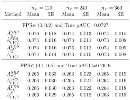
Comparison of SPEL-pAUC and competing methods . . . .
67
3.2
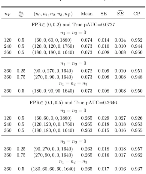
Properties of the SPEL-pAUC
. . . .
68
3.3
Comparison of SPEL-pAUC and competing methods for Chi-Squared
Dis-tributed Data . . . .
69
3.4
Descriptive statistics for the Balcone risk score . . . .
69
3.5
Sample allocation for the non-small-cell lung cancer data . . . .
69
3.6
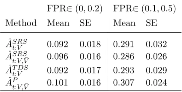
Descriptive statistics for FFN . . . .
69
3.7
Sample allocation for the Preterm Prediction Study
. . . .
70
4.1
Comparison of SPEL-ROC and competing methods . . . .
89
4.2
SPEL-ROC for specific covariate values
. . . .
90
4.3
Properties of the SPEL-ROC . . . .
92
4.4
Descriptive statistics for the Balcone risk score and age of patients . . . .
93
LIST OF TABLES
2.1
Comparison of SPEL-AUC and competing methods . . . .
44
2.2
Asymptotic results for SPEL-AUC . . . .
45
2.3
Comparison of SPEL-AUC and competing methods for Chi-Squared Distributed
Data . . . .
45
2.4
Descriptive statistics for the Balcone risk score . . . .
46
2.5
Sample allocation for the non-small-cell lung cancer data . . . .
46
2.6
Descriptive statistics for FFN . . . .
46
2.7
Sample allocation for the Preterm Prediction Study
. . . .
46
3.1
Comparison of SPEL-pAUC and competing methods . . . .
67
3.2
Properties of the SPEL-pAUC
. . . .
68
3.3
Comparison of SPEL-pAUC and competing methods for Chi-Squared
Dis-tributed Data . . . .
69
3.4
Descriptive statistics for the Balcone risk score . . . .
69
3.5
Sample allocation for the non-small-cell lung cancer data . . . .
69
3.6
Descriptive statistics for FFN . . . .
69
3.7
Sample allocation for the Preterm Prediction Study
. . . .
70
4.1
Comparison of SPEL-ROC and competing methods . . . .
89
4.2
SPEL-ROC for specific covariate values
. . . .
90
4.3
Properties of the SPEL-ROC . . . .
92
4.4
Descriptive statistics for the Balcone risk score and age of patients . . . .
93
tributed Data . . . .
69
3.4
Descriptive statistics for the Balcone risk score . . . .
69
3.5
Sample allocation for the non-small-cell lung cancer data . . . .
69
3.6
Descriptive statistics for FFN . . . .
69
3.7
Sample allocation for the Preterm Prediction Study
. . . .
70
4.1
Comparison of SPEL-ROC and competing methods . . . .
89
4.2
SPEL-ROC for specific covariate values
. . . .
90
4.3
Properties of the SPEL-ROC . . . .
92
4.4
Descriptive statistics for the Balcone risk score and age of patients . . . .
93
4.5
Sample allocation for the non-small-cell lung cancer data . . . .
93
4.6
Lung Cancer Study: Comparison of Covariate-specific ROC Curve Estimators
94
LIST OF TABLES
2.1
Comparison of SPEL-AUC and competing methods . . . .
44
2.2
Asymptotic results for SPEL-AUC . . . .
45
2.3
Comparison of SPEL-AUC and competing methods for Chi-Squared Distributed
Data . . . .
45
2.4
Descriptive statistics for the Balcone risk score . . . .
46
2.5
Sample allocation for the non-small-cell lung cancer data . . . .
46
2.6
Descriptive statistics for FFN . . . .
46
2.7
Sample allocation for the Preterm Prediction Study
. . . .
46
3.1
Comparison of SPEL-pAUC and competing methods . . . .
67
3.2
Properties of the SPEL-pAUC
. . . .
68
3.3
Comparison of SPEL-pAUC and competing methods for Chi-Squared
Dis-tributed Data . . . .
69
3.4
Descriptive statistics for the Balcone risk score . . . .
69
3.5
Sample allocation for the non-small-cell lung cancer data . . . .
69
3.6
Descriptive statistics for FFN . . . .
69
3.7
Sample allocation for the Preterm Prediction Study
. . . .
70
4.1
Comparison of SPEL-ROC and competing methods . . . .
89
4.2
SPEL-ROC for specific covariate values
. . . .
90
4.3
Properties of the SPEL-ROC . . . .
92
4.4
Descriptive statistics for the Balcone risk score and age of patients . . . .
93
tributed Data . . . .
69
3.4
Descriptive statistics for the Balcone risk score . . . .
69
3.5
Sample allocation for the non-small-cell lung cancer data . . . .
69
3.6
Descriptive statistics for FFN . . . .
69
3.7
Sample allocation for the Preterm Prediction Study
. . . .
70
4.1
Comparison of SPEL-ROC and competing methods . . . .
89
4.2
SPEL-ROC for specific covariate values
. . . .
90
4.3
Properties of the SPEL-ROC . . . .
92
4.4
Descriptive statistics for the Balcone risk score and age of patients . . . .
93
4.5
Sample allocation for the non-small-cell lung cancer data . . . .
93
4.5
Sample allocation for the non-small-cell lung cancer data . . . .
93
4.6
Lung Cancer Study: Comparison of Covariate-specific ROC Curve Estimators
94
4.7
Preterm Prediction Study: Descriptive Statistics for FFN and Cervical Length
94
4.8
Sample allocation for the Preterm Prediction Study
. . . .
95
4.9
Preterm Prediction Study: Comparison of Covariate-specific ROC Curve
Esti-mators . . . .
96
4.7
Preterm Prediction Study: Descriptive Statistics for FFN and Cervical Length
94
4.8
Sample allocation for the Preterm Prediction Study
. . . .
95
4.9
Preterm Prediction Study: Comparison of Covariate-specific ROC Curve
LIST OF FIGURES
1.1
Area under the ROC curve
. . . .
6
1.2
Partial area under the ROC curve
. . . .
6
4.1
Covariate-specific ROC Curve . . . .
91
4.2
Lung Cancer Study: SPEL-ROC by Age . . . .
95
4.3
Preterm Prediction Study: SPEL-ROC by Cervical Length
. . . .
97
LIST OF FIGURES
1.1
Area under the ROC curve
. . . .
6
1.2
Partial area under the ROC curve
. . . .
6
4.1
Covariate-specific ROC Curve . . . .
91
4.2
Lung Cancer Study: SPEL-ROC by Age . . . .
95
LIST OF ABBREVIATIONS
AUC
Area under the ROC curve
CL
Cervical length
FFN
Fetal Fibronectin
FPR
False positive rate
LS-ROC
Least squares ROC curve estimator
MW-AUC
Mann-Whitney AUC estimator
NP-pAUC
Nonparametric partial AUC estimator
NPEL-AUC
Nonparametric empirical likelihood AUC estimator
NPEL-pAUC
Nonparametric empirical likelihood partial AUC estimator
NSCLC
Non-small cell lung cancer
ODS
Outcome dependent sample
pAUC
Partial area under the ROC curve
PPS
Preterm Prediction Study
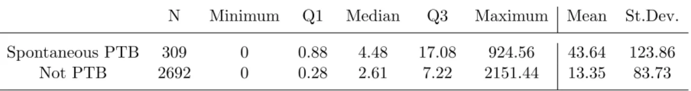
PTB
Preterm birth
ROC
Receiver operating characteristic
SE
Standard error
SPEL-AUC
Semi-parametric empirical likelihood AUC estimator
SPEL-pAUC
Semi-parametric empirical likelihood pAUC estimator
SPEL-ROC
Semi-parametric empirical likelihood covariate-specific ROC curve estimator
SRS
Simple random sampling
TDS
Test-dependent sampling
TPR
True positive rate
LIST OF ABBREVIATIONS
AUC
Area under the ROC curve
CL
Cervical length
FFN
Fetal Fibronectin
FPR
False positive rate
LS-ROC
Least squares ROC curve estimator
MW-AUC
Mann-Whitney AUC estimator
NP-pAUC
Nonparametric partial AUC estimator
NPEL-AUC
Nonparametric empirical likelihood AUC estimator
NPEL-pAUC
Nonparametric empirical likelihood partial AUC estimator
NSCLC
Non-small cell lung cancer
ODS
Outcome dependent sample
pAUC
Partial area under the ROC curve
PPS
Preterm Prediction Study
PTB
Preterm birth
ROC
Receiver operating characteristic
SE
Standard error
SPEL-AUC
Semi-parametric empirical likelihood AUC estimator
SPEL-pAUC
Semi-parametric empirical likelihood pAUC estimator
SPEL-ROC
Semi-parametric empirical likelihood covariate-specific ROC curve estimator
SRS
Simple random sampling
TDS
Test-dependent sampling
Chapter 1
Literature Review
1.1
Introduction and motivation
Using statistical tools to discriminate between different populations is beneficial in a wide
variety of areas. One such tool is the receiver operating characteristic (ROC) curve, which
was developed for electronic signal detection (Hanley, 1989). The diagnostic methods have
been expanded to be useful in a wide variety of medical applications: from medical imaging
techniques (Swets, 1979) and studying risk markers for cardiovascular disease (Yeboah et al.,
2012) to using prostate-specific antigen to detect prostate cancer (Dodd and Pepe, 2003b)
and applying time-dependent accuracy summaries in the setting of survival analysis models
(Heagerty and Zheng, 2005). There is also a wide variety of statistical methods proposed in
this area: from new summary measurements to methods of dealing with missing data in this
diagnostic setting and changing the way in which subjects are sampled into the study.
Receiver operating characteristic (ROC) curves and area under the ROC curve (AUC) are
summary measures used to describe the ability of a screening test to discriminate between
diseased and non-diseased subjects (Bamber, 1975). As evaluating the true disease status can
be costly, it is beneficial for researchers to increase study efficiency by allowing selection
prob-abilities to depend on the screening test (Wang et al., 2012). Increased efficiency translates
to cost and time savings for studies as well as decreased burden on subjects.
Consider screening for non-small-cell lung carcinoma (NSCLC) cancer recurrence. Lung
cancer is the most common cause of cancer death among men and women in the world
or non-small-cell lung carcinoma (NSCLC), of which NSCLC accounts for approximately 80%
of all lung cancers. After surgical lung resection, a large proportion of stage 1 NSCLC patients
have cancer recurrence within five years (Bueno et al., 2012). When surgery is used as the
primary treatment for NSCLC, adjuvant chemotherapy may benefit patients who have a high
risk of cancer recurrence.
Identifying patients who are at high risk of cancer recurrence
is important in order for treatment to be given to those who would benefit most. This is
an important area of study for patients, families, and doctors when making decisions on a
treatment plan.
We used data from the data from the CALGB 150807 study conducted by the Cancer and
Leukemia Group B (Bueno et al., 2012). This study is a subset of patients registered in the
CALGB 140202 study who have stage 1A or 1B non-small-cell lung cancer (NSCLC). Among
patients in the CALGB 150807 study, 1,061 patients were not censored before 12 months
and were used in this analysis. The Balcone risk score, outlined by Blanchon et al. (2006),
has been developed to identify patients who are at greatest risk of cancer recurrence. The
risk score is developed by considering factors such as age, gender, activity level at diagnosis,
histological type, and the tumor-node-metastasis staging system.
There are many interesting questions that can be explored in this study. AUC can be
used to investigate the ability of the Balcone risk score to predict cancer recurrence. Given
the need for an accurate test, partial AUC (pAUC) can be used to evaluate the performance
of the Balcone risk score where a specific range of FPRs or TPRs is considered. Because large
FPRs are less clinically relevant, we can restrict the range of interest to FPR
∈
(0,
0.3), for
example. With the wealth of patient information available, a covariate-specific ROC would
allow us to evaluate the performance of the Balcone risk score, while accounting for covariates
that appear to be associated with cancer recurrence. This covariate-specific ROC estimator
can then be used to identify subsets of the population where the screening test is better at
distinguishing between subjects who have cancer recurrence and those who do not.
There have been many methods studied and proposed in the area of ROC and AUC
analysis. Bamber (1975) proposed a nonparametric AUC estimator, which is equivalent to
Swets and Pickett (1982) and Hanley et al. (1983). These methods use SRS for selection
into the study. Wang et al. (2012) proposed a nonparametric AUC estimator which utilizes
a biased sampling design in order to target subjects who contribute more information to the
study. McClish (1989) and Thompson and Zucchini (1989) introduced the idea of evaluating
only part of the AUC when a subset of FPRs are of interest. The pAUC can be interpreted
as the joint probability that
Y
D> Y
D¯and
Y
D¯fall within the FPR range of interest (Dodd
and Pepe, 2003a). Estimators similar to those given above for the AUC have been proposed
for the pAUC. A nonparametric pAUC estimator that uses SRS data was proposed by Dodd
and Pepe (2003a) and a nonparametric pAUC estimator using a biased sampling scheme
was proposed by Wang et al. (2012). Another discriminatory measure used to differentiate
between two populations when data are available over time is the C statistic (Rizopoulos,
2011; Pencina et al., 2012b; Heagerty and Zheng, 2005; Antolini et al., 2005). The C statistic
is a weighted average of the AUCs across multiple time points in the study. Heagerty and
Zheng (2005) suggested that the time specific AUCs can be plotted over time to assess changes
in accuracy across time for a time to event outcome.
Another important area of research the use of covariates in modeling ROC and in
esti-mating AUC and pAUC. The use of covariates allows us to better understand the influence
covariates have on accuracy of the screening test (Wang et al., 2013). Thompson and Zucchini
(1989) proposed nonparametric direct estimation of the AUC for specific level of a categorical
covariate. Wang et al. (2013) proposed ROC estimation which uses a biased sampling design
and a binormal model for screening test variable. Dodd and Pepe (2003a,b) proposed using
a generalized linear model framework for modeling the screening test, which can be used to
estimate AUC and pAUC.
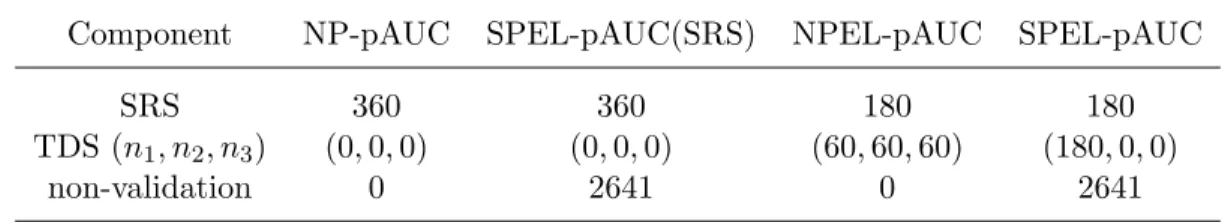
The proposed work focuses on estimation of AUC, pAUC, and a covariate-specific ROC
curve using biased sampling methods and all available information, including incomplete
information available for un-sampled subjects. We consider a test dependent sampling (TDS)
design where TDS inclusion is dependent on a continuous screening test measure. Here,
the Balcone risk score is the measure used for the biased sampling scheme. This biased
un-sampled subjects as opposed to a design using only a simple random sample of the same
size. The idea behind the supplemental sample is to target resources where the greatest
amount of information can be attained (Zhou et al., 2002). Cancer recurrence and other
covariate information are known only for those included in the SRS and TDS components.
The screening test measure and other baseline information are available for all subjects in the
study. Information from un-sampled subjects will also be utilized in the proposed methods.
Using the biased sampling design as well as incorporating observed information from the
un-sampled subjects can lead to efficiency improvements. This suggests that a smaller sample
size can be used with these methods, compared to existing methods, where a larger sample
size would be necessary to obtain the same level of efficiency in the estimator. A smaller
sample size translates to cost savings for the study and decreased subject burden. Using this
biased sampling design, we propose multiple approaches to studying these data that answer
different questions, which are helpful in understanding the utility of the screening test.
1.2
ROC Curves and Area under the ROC curve (AUC)
1.2.1
Unadjusted methods
There are many ways to approach the use of data in the area of medical decision making.
Methods have been proposed for a variety of types of estimators. Greenhouse and Mantel
(1950) suggested that to be considered an acceptable test, a screening test should be able to
correctly classify at least a pre-specified percentage of the diseased subjects and incorrectly
classify no more than a set percentage who are well. Other common measures include area
under the ROC curve (AUC) and partial AUC, where a particular interval of FPRs or TPRs
are of interest. A three dimensional extension of ROC and AUC was proposed by Skaltsa
et al. (2012), where instead of a two level outcome (diseased or not diseased) the outcome can
have more levels. This is beneficial for studying diseases such as Alzheimer’s disease. In this
case, the disease naturally presents with a transition state that falls between normal aging
and irreversible Alzheimer’s disease, which can be described as mild cognitive impairment. Yu
for a missing outcome or diagnostic screening variable without eliminating those subjects
from the analysis, limiting bias and loss in efficiency. Wang et al. (2012, 2013) suggested
an alternate approach to sampling subjects in order to target those who contribute more
information. With this biased sampling scheme, a smaller sample size can be used to attain
estimates that are as good as or better than alternative sampling methods, such as SRS.
ROC and AUC
The receiver operating characteristic (ROC) curve is a tool used to display how well a
screening test,
Y
, is able to indicate disease status,
D. The ROC curve is constructed by
plotting the false positive rate (FPR,
P r
(Y
≥
c
|
D
= 0)) versus the true positive rate (TPR,
P r
(Y
≥
c
|
D
= 1)), where c is the threshold for the screening test to indicate disease. The area
under the ROC curve (AUC) is a summary measure used to determine both the importance
of a difference between two populations and also describes the accuracy of discrimination
performance (Bamber, 1975). Figure 1.1 shows an ROC curve with corresponding AUC. The
FPR and TPR range from 0 to 1, and the AUC ranges from 0.5 to 1. An ROC curve with
intercept 1 and slope 0 indicates a perfect screening test that correctly identifies disease status
in every subject. An ROC curve with intercept 0 and slope 1, creating a 45
oline, indicates
a screening test that is essentially as good as flipping a coin. A screening test with an ROC
curve that falls above the 45
oline indicates some level of ability of the screening test to
discriminate between diseased and non-diseased subjects.
Another summary measure is the partial AUC (pAUC), shown in Figure 1.2. The pAUC
restricts the FPR (or TPR) to a range that is more clinically relevant.
McClish (1989)
and Thompson and Zucchini (1989) introduced the idea of evaluating only part of the AUC
for certain FPR intervals that are of interest. The pAUC can be interpreted as the joint
probability that
Y
D> Y
D¯and
Y
D¯fall within the FPR range of interest (Dodd and Pepe,
2003a). There are downsides that must be considered when using the pAUC. The standard
error of the pAUC estimator increases and there is a loss in precision when a major restriction
Figure 1.1: Area under the ROC curve
Figure 1.2: Partial area under the ROC
curve
AUC and pAUC estimators
A binormal model for estimating AUC was proposed by Swets and Pickett (1982) and
Hanley et al. (1983). They compared the binormal model for estimating AUC to the
non-parametric AUC estimator. Swets and Pickett (1982) suggested that the method
assum-ing a binormal model for the screenassum-ing test variable is superior to the nonparametric
es-timator because with the binormal model, the eses-timator is less affected by location and
spread of points that define the ROC. The area under the empirical ROC curve is given by
ˆ
A
SRS=
n 1DnD¯
P
nD¯j=1
P
nDi=1
I Y
Di> Y
Dj¯+
21I Y
Di=
Y
Dj¯, which is the Mann-Whitney
U-statistic (Bamber, 1975). Both of these approaches to estimating the AUC use data that are
sampled from the population with SRS.
Dodd and Pepe (2003a) extended this AUC estimator in the SRS setting for pAUC. The
proposed pAUC estimator restricts the FPR (or TPR) and is given by
ˆ
A
SRSt=
1
n
Dn
D¯ nX
i=1 n
X
j=1
D
i(1
−
D
j)
I
(Y
i> Y
j, Y
j∈
(q
0, q
1))
where
q
0=
F P R
−1(t
1) and
q
1=
F P R
−1(t
0). This estimator is nonparametric and shows
only moderate efficiency compared to parametric estimators. For the FPR component of the
estimator, they found that using the estimated quantiles instead of the true quantiles gave
improved efficiency for estimating pAUC (Dodd and Pepe, 2003a).
An empirical likelihood method for estimating AUC was proposed by Qin and Zhou (2006).
This estimator showed improved small sample properties compared to assuming a normal
ap-proximation. A confidence interval for the AUC was also developed. The empirical likelihood
methods made it possible to obtain estimates for parameters without specifying a distribution
for the screening test. To obtain confidence intervals, they showed that their proposed AUC
estimator followed a scaled chi-square distribution, giving asymptotically correct coverage
probability. Although these methods were derived for a SRS, the methods can be extended
to account for a stratified sampling design. McNeil et al. (1984) developed methods when a
fixed FPR or TPR are of interest. These methods assumed normality of the screening test
variable.
TDS methods
Wang et al. (2012) proposed estimators for both AUC and pAUC that improve efficiency by
using a biased sampling design. These estimators are nonparametric and show improvement
over the simple random sampling setting when using the standard AUC estimator and the
pAUC estimator proposed by Bamber (1975) and Dodd and Pepe (2003a), respectively. The
form of these estimators is similar to that of the SRS estimators, but weights are incorporated
that account for the biased sampling design. The AUC and pAUC estimators proposed by
Wang et al. (2012) are given by:
ˆ
A
T DS=
P
n i=1P
nj=1
p
ip
jD
i(1
−
D
i)
I
(Y
i> Y
j)
P
ni=1
P
nj=1
p
ip
jD
i(1
−
D
i)
ˆ
A
tT DS
=
P
n i=1P
nj=1
p
ip
jD
i(1
−
D
i)
I
Y
i> Y
j, Y
j∈
F P R
ˆ
P
n i=1P
nj=1
p
ip
jD
i(1
−
D
i)
where the false positive rate is estimated by
F P R
ˆ
j=
P
ipˆi(1−Di)I(Yi>Yj) P
ipˆi(1−Di)
. In Wang et al.
(2012), the TDS methods described for AUC and pAUC were used in evaluating the survival
is a protein that is over-expressed with lung cancer. Its intensity ranges from 0 to 10, and it
stratified into three groups to obtain the TDS portion of the sample: negative (COX-2
<
2),
moderate (2
≤
COX-2
<
4), and positive (COX-2
≥
4). Preliminary data showed that the
proportions of patients falling into these categories were approximately 60%, 13%, and 27%,
respectively. In order to study the relationship between COX-2 value and survival, a range of
COX-2 values needs to be seen. Because treating and tracking outcomes for subjects is costly,
a sample is usually taken in order to complete the study on a fixed budget. The TDS method
for sampling was implemented in order to select enough subjects with moderate and positive
COX-2 to study this relationship. Define
D
= 1 as patients who survive less than 6 years
and
D
= 0 otherwise. Targeting a small range for the FPR can be important as false positive
results add increased cost and burden on subjects. With this in mind, the FPR interval of
interest was (0,
0.1). More details in the biased sampling component for this estimator are
given later in the Outcome-Dependent-Sampling portion of the literature review.
1.2.2
Covariate adjusted methods
Methods have been developed which consider the effect of covariate information on ROC
curves. This can be accomplished in many ways, such as estimating the covariate effect
on the screening test, directly estimating the AUC, and directly estimating the covariate
specific ROC curve. Tosteson and Begg (1988) proposed modeling the effect of covariates on
the screening test,
Y
. Here, a distribution function was assigned for
Y
, and the resulting
covariate effect on the ROC curve was calculated.
There are limitations here, as model
misspecification can lead to erroneous results. Thompson and Zucchini (1989) and Dodd and
Pepe (2003a) proposed directly estimating the AUC, and Dodd and Pepe (2003a) proposed
directly estimating pAUC, while accounting for covariates. Methods for directly estimating
the survival function or the ROC curve were proposed by Pepe (1997, 2000), Cai and Pepe
(2002), and Wang et al. (2013). Generalized linear modeling methods were used in Pepe
(1997, 2000). These results were extended to a semi-parametric approach by Cai and Pepe
Thompson and Zucchini (1989) proposed that estimation can be completed by specifying
a distribution function for
Y
or can be completed nonparametrically using the Wilcoxon
statistic:
AU C
ˆ
k=
n
−D,k1n
−D,k¯1P
nD,ki
P
nD,k¯i
{
I
[Y
j< Y
i] + 0.5I
[Y i
=
Y
j]
}
, where
k
= 1, . . . , K
denotes the covariate level. Thompson and Zucchini (1989) also proposed an analysis of
variance (ANOVA) approach for modeling to compare the means of an accuracy index for
different combinations of variables. In this setting, images are read by multiple people and
these results are compared to see how ratings compare between readers. The model is given
by
Y
ijk=
µ
+
α
i+
b
j+ (ab)
ij+
c
+
e
ijk, where
µ
+
α
irepresents the mean level of Y for the
i-th combination of the variables. The variable
b
jis a random variable, allowing for variation
between image readers. Zheng and Heagerty (2007) proposed a semi-parametric estimate
of the survival function of the screening test over time. The ROC is constructed from this
estimated survival function, and AUC can be assessed over time. The added component of
following a subject’s screening test variable over time allows for the ability to assess diagnostic
accuracy at different intervals of time between measurement and diagnosis.
Methods to estimate the AUC and pAUC while adjusting for covariates provide useful
model interpretations for both discrete and continuous covariates (Dodd and Pepe, 2003a,b).
These methods are semi-parametric and take advantage of generalized linear model
frame-work. Dodd and Pepe (2003b) define the covariate specific AUC as
P r
Y
iD> Y
jD¯|
X
iD, X
jD¯=
θ
ij. The regression model is given by
g
(θ
ij) =
X
Tijβ
, where
β
is a vector of parameters and
g
is a monotone increasing link function.
The proposed estimating function is given by
S
N(β) =
P
niDP
njD¯ ∂θ∂βijv
(θ
ij)
−1(U
ij−
θ
ij)
≡
P
inDP
njD¯S
ij(
β
). Dodd and Pepe (2003a)
propose the covariate-specific pAUC given by
AU C
X(t
0, t
1)
=
P r
Y
D> Y
D¯, Y
D¯∈
(q
0, q
1)
|
X
.
The general model is given by
AU C
X(t
0, t
1) =
g X
Tβ
for a specified link function
g. For
the pAUC setting the estimating equation is given by
V
nD,nD¯(β)
=
nD
X
i nD¯
X
j
∂θ
X∂β
v
(θ
X)
−1
V
(q0,q1)ij
−
θ
Xwhere
V
(q0,q1)ij
=
I
Y
iD> Y
jD¯, Y
jD¯∈
(q
1, q
0)
.
When using the logit link, exponentiated
model parameters can be interpreted as AUC or pAUC odds. For a binary covariate, the
exponentiated model parameter can be interpreted as the ratio of AUC or pAUC odds
be-tween the two levels of that covariate. For a continuous covariate, the exponentiated model
parameter can be used to describe how AUC or pAUC changes for diseased and not
dis-eased subjects as that covariate changes. Dodd and Pepe (2003b) used their proposed AUC
methods to study the ability of the distortion product otoacoustic emission (DPOAE)
de-vice in assessing impaired hearing. The DPOAE dede-vice is used at three different frequencies
and three intensity settings, creating nine combinations of settings. The severity of hearing
loss is also of interest in this setting. A behavioral test where subjects indicate the point
at which a sound is audible is the gold standard in assessing hearing loss. The model used
here is given by
log
1−AU CAU C=
β
0+
β
1intensity
+
β
2f requency
+
β
3severity. Results from
this analysis showed that DPOAE is able to discriminate between severely impaired ears and
normal ears better than mildly impaired and normal ears, which is not surprising. Also,
stimuli with lower intensities achieved greater accuracy. Dodd and Pepe (2003a) considered
the ability of prostate-specific antigen (PSA) to diagnose prostate cancer. The data came
from the
α-Tocopheraol and
β-Carotene Study (ATBC). Serum samples were collected and
stored at baseline and three years later. Adjusting for time was important here, especially
because the time from measurement to diagnosis varied greatly and it was expected that
PSA levels taken close to the time of diagnosis would be more predictive. Clinical evidence
showed a relationship between PSA levels and prostate cancer. Two methods of quantifying
PSA were considered, total PSA and the ratio of free to total PSA. The comparison of these
two methods was incorporated into the model. Ultimately, 240 subjects in the study were
diagnosed with prostate cancer during the eight year study follow-up period. Serum samples
were age matched for 237 non-prostate diagnosed subjects who were sampled for comparison.
They considered FPR values in (0,
0.4). The model was given by:
log
AU C
(0,
0.4)
0.4
−
AU C
(0,
0.4)
The results showed that PSA accuracy improved when subjects were measured at times closer
to the time of diagnosis. Total PSA appeared to be a better diagnostic tool for prostate cancer
than the ratio.
Pepe (1997) proposed a regression design that directly modeled covariate effects on the
ROC curve. Denote
D
the binary indicator of disease status,
Y
the non binary diagnostic test,
Z
the factors that potentially influence test accuracy, and
X
the vector of covariates. The
ROC curve associated with
Z
for a logistic model is given by
ROC
Z(t) =
1+expexp{α{0α(t)+0(t)+XβXβ}},
where
α
0(t) is a monotone function from (0,
1) to (
−∞
,
∞
), and
t
denotes the false positive
rate. No distributional assumptions are made for
Y
; assumptions are made only for the
relationship between diseased and non diseased subjects through the ROC curve model. This
approach allows for examining the influence covariates have on the accuracy of a diagnostic
test in discriminating disease status. This method was applied to radiology data, the same
used in Thompson and Zucchini (1989), where images were constructed and then evaluated
by three readers. Here, there were 50 each of diseased and non diseased images and the
readers classified their evaluation of each image with an ordinal scale from 1 to 5. After
data collection, the 4
thand 5
thcategories were collapsed due to sparse data. A logistic
type regression was fit to the data with the model
ROC
Z(t) =
exp{α0(t)+β1X1+β2X2+β3X3}
1+exp{α0(t)+β1X1+β2X2+β3X3}
,
where
X
icorresponds to the evaluation made by the
i
threader. This technique allowed for
comparisons between readers, such as reader 3 rating images systematically lower than the
other two readers.
An ROC curve estimator was proposed by Wang et al. (2013), which uses test dependent
sampling (TDS), a biased sampling design. With this method, portions of the population
are oversampled to gain efficiency. A binormal model is assumed for the screening test,
Y
,
such that
Y
=
β
0+
β
DD
+
β
XTX
+
β
DXTDX
D+
σ
(D)
, where
∼ N
(0,
1) and
σ
(D) =
σ
1I
[D
= 1] +
σ
0[D
= 0]. No distributional assumptions are needed for the covariates due to
the use of empirical likelihood methods. Estimates of the survival function were estimated
and combined for a covariate-specific ROC curve, given by:
ROC
X(t) =
S
1XS
1X−1(t)
=
Φ
βD+βDXT XD+σ0Φ−1(t)
σ1
.
This method was applied to data from a study evaluating the
et al. (2012). Covariates such as age and gender were included in the model. These covariates
not only have a relationship with cancer survival, but also on the COX-2 expression, so
ability to include these covariates in the study is valuable. Simulation studies showed that
the estimator will perform fairly well under mild misspecification of the binormal model.
Other summary measures
Another discriminatory measure used to differentiate between two populations is the C
statistic (Rizopoulos, 2011; Pencina et al., 2012b; Heagerty and Zheng, 2005; Antolini et al.,
2005). In situations such as survival analysis settings, time dependent ROC and AUC can
be used to evaluate the screening test over time. Rizopoulos (2011) described the C statistic
as a summary of the screening test variable over the study period. This weighted average
of the AUCs is given by
C
=
R
AU CtP r
(
Ti∗>t)
dt RP r
(
Ti∗>t)
dt, where
P r
(T
∗i
> t) is the marginal survival
probability. The marginal survival probability takes into account censoring, since all time
points will not contribute equally. Heagerty and Zheng (2005) suggested that the time
spe-cific AUCs can be plotted over time to assess a change in accuracy across time. While the
methods proposed by Heagerty and Zheng (2005) and Rizopoulos (2011) are semiparametric,
the methods proposed by Antolini et al. (2005) are non-parametric making them more robust.
Missing data
Instead of focusing of new types of summary measures for discrimination between
popula-tions, Yu et al. (2011), Liu and Zhou (2011), and Long et al. (2011b,a) considered the common
issue of missing data. Long et al. (2011b,a) developed methods for missing screening test
val-ues. Loss of efficiency and, depending on the type of missingness, bias may be introduced
when only including subjects with complete data. Both missing at random and missing not at
random scenarios are considered. This AUC estimator was shown to work well under model
misspecification. Nonparametric imputation procedures were used in developing methods to
analyze ROC when the biomarker for screening was missing. In this case, other auxiliary
variables were present and were used in imputing the main biomarker of interest. Instead of
the absence of the screening test variable, Yu et al. (2011) and Liu and Zhou (2011) developed
combined multiple continuous tests together as a composite test to discriminate between two
populations. It was assumed that the test values are binormal, and a Bayesian latent disease
model was used, along with an MCMC algorithm for computation. Glomerular filtration rate
(GFR) is a measurement associated with the ability of the kidneys to filter. A reduced GFR
is a marker for chronic kidney disease. Chronic kidney disease is defined as kidney damage
or GFR measurement below a set threshold. There are different ways to estimate the GFR
and no true gold standard in defining chronic kidney disease. Methods proposed by Yu et al.
(2011) were used to assess the optimal way of measuring GFR to diagnose chronic kidney
dis-ease. Liu and Zhou (2011) developed a semiparametric ROC curve estimator where the gold
standard is missing for a subset of the study population. The missing at random assumption
was assumed in the development of these estimators. Weighted estimating equations were
used to account for the missing gold standard for a subset of the subjects.
Optimal threshold for Y
Another interesting and important research topic in the area of ROC and AUC is
choos-ing the best threshold value of the screenchoos-ing test to indicate disease. Different approaches
can be considered in finding the optimal threshold for the screening test and in assessing
improvement in the screening tests available. Molanes-L´
opez and Let´
on (2011) used
empir-ical likelihood methods to assess the most appropriate cut-off value for the diagnostic test
using the Youden index. The nonparametric empirical likelihood methods were compared to
a newly developed parametric methods. Simulation studies showed that the nonparametric
method was competitive with other parametric methods and was superior. Pencina et al.
(2012a) evaluated the improvement in population discrimination using AUC. These methods
assume multivariate normality and use a linear discriminant analysis. The measures under
study reduce to a function of Mahalanobis distance, which helps to describe the magnitude of
improvement in estimation. Let
M
p+q2=
δ
TΣ
−1δ
denote the Mahalanobis distance for
p
+
q
cases. The first of the three estimators proposed was assessing the change in AUC, ∆AU C.
This estimator reduces to ∆AU C
= Φ
q
M2p+q
2
−
Φ
q
M2p
2