Messier_unc_0153D_15170.pdf

(1)

SPATIOTEMPORAL GEOSTATISTICAL METHODS FOR EXPOSURE AND EPIDEMIOLOGICAL ANALYSES OF GROUNDWATER NITRATE AND RADON

Kyle Philip Messier

A dissertation submitted to the faculty of the University of North Carolina at Chapel Hill in partial fulfillment of the requirements for the degree of Doctor of Philosophy in the Department

of Environmental Sciences and Engineering of the Gillings School of Global Public Health.

Chapel Hill 2015

Approved by: Marc L. Serre Rebecca C. Fry

Jacqueline A. MacDonald Gibson Lawrence E. Band

(2)

(3)

iii

ABSTRACT

Kyle P Messier: Spatiotemporal Geostatistical Methods for Exposure and Epidemiological Analyses of Groundwater Nitrate and Radon

(Under the Direction of Marc L. Serre)

Exposure assessment and dose-response characterization are critical steps in the risk assessment of an environmental contaminant with potential human health effects. There are many established methods to conduct exposure assessments and to characterize the dose-response relationship between a contaminant of concern and a health outcome; however, many require extensive time and monetary resources that are becoming increasingly limited.

Geostatistical methods are attractive approaches due to their cost-effective implementation and clear physical interpretations. Land use regression (LUR) is a type of geostatistical method that uses spatially-based explanatory variables to model outcomes using classical regression methods. Bayesian Maximum Entropy (BME) is a geostatistical framework for incorporating

measurements as well as various knowledge bases in a logical and theoretically sound manner to produce estimates for variables of interest at unmonitored locations. This work advances these spatiotemporal geostatistical methods in the following three studies: 1) An exposure assessment of groundwater nitrate (𝑁𝑂₃−), a biological nutrient with natural and anthropogenic sources that in excess has deleterious effects on human and ecological health; 2) An exposure assessment of groundwater radon (222𝑅𝑛), a naturally occurring gas with radioactively discharged alpha particles that are known human carcinogens; and 3) An epidemiological analysis of the association between groundwater 222𝑅𝑛exposure and lung and stomach cancer incidence.

First, we develop a nonlinear LUR model and then integrate the model into the BME framework to produce the first space/time exposure estimates of groundwater 𝑁𝑂₃−

(4)

uranium-iv

based explanatory variables resulting in a cross-validation 𝑟2of 0.46. Lastly, we utilize the LUR-BME exposure model for 222𝑅𝑛to investigate associations with lung and stomach cancer at multiple spatial scales. It is the first epidemiological analysis of the association between groundwater 222𝑅𝑛 exposure and lung cancer, moreover with a significant and positive

(5)

v

For my late mother

Janice Irwin Messier

(6)

vi

ACKNOWLEDGEMENTS

I would first like to thank my advisor, Dr. Marc L. Serre, for bringing me into his lab and providing excellent mentorship through both a Master’s and PhD. We had many a fruitful discussions ranging from technical statistics to abstract philosophy and international soccer matches. I am grateful to call Marc a mentor, a colleague, and a friend.

I would also like to thank my committee members, Dr. Rebecca C. Fry, for valuable research advice and for providing PhD funding for two years; Dr. Jacqueline A. MacDonald Gibson, for valuable input and research advice; Dr. Lawrence E. Band, for research advice and his excellent course covering the excitable research area of nitrogen; and Dr. Gregory W. Characklis, for reviewing and editing many papers and abstracts. I would also like to thank Dr. Leena Nylander-French for providing funding for two years during my PhD.

I would like to thank my friends in the department for making my time as a graduate student not only a valuable time professionally, but also socially. It was great to have many friends in the window-less, tornado bunker better known as the Rosenau basement. And of course I cannot forget our amazingly mediocre intramural basketball team. I still feel sorry for the referees.

(7)

vii

LIST OF TABLES

Table 1.1. Leave-one-out cross-validation statistics comparing nitrate models. ...24

Table 1.2. Nonlinear regression model variables selected via CFN-RHO and parameter estimates for time-averaged nitrate monitoring and private well models. ...25

Table S1.1. Groundwater Nitrate Data Source Basic Information. ...46

Table S1.2. Spatial explanatory variable model categories. ...46

Table S1.3. Nonlinear regression model variables selected via CFN-RHO ...47

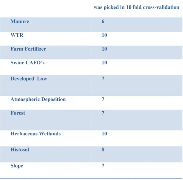
Table S1.4. The number of times each variable in the full spatially-smoothed/time-averaged LUR model for monitoring wells was selected in the ten-fold cross-validation runs. ...48

Table S1.5. The number of times each variable in the full spatially-smoothed/time-averaged LUR model for private wells was selected in the ten-fold cross-validation runs. ...49

Table S1.6. The number of times each variable in the full time-averaged LUR model for monitoring wells was selected in the ten-fold cross-validation runs. ...50

Table S1.7. The number of times each variable in the full time-averaged LUR model for private wells was selected in the ten-fold cross-validation runs. ...50

Table S1.8. Comparison of area within study area predicted by monitoring and private well LUR-BME model concentrations above a threshold ...51

Table S1.9. Comparison of area within study area predicted by Nolan and Hitt 2006 GWAVA monitoring and drinking-water model concentrations above a threshold ...52

Table 2.1. Land Use Regression model selected through A Distance Decay Regression Selection Strategy. ...74

Table 2.2. Leave-One-Out Cross-Validation statistics for the radon LUR, BME, and LUR-BME methods...76

(12)

xii

Table 3.2. Lung Cancer Negative Binomial regression results for

groundwater radon concentration for multiple models. ...109 Table 3.3. Lung cancer logistic GLM results representing the odds

a case is within the lung cancer cluster. ...110 Table 3.4. Stomach cancer logistic GLM and GEE results representing

the odds that a stomach cancer case falls within a local

stomach cancer cluster. ...111 Table S3.1. Lung cancer negative binomial regression models for

groundwater radon and all confounding variables.. ...129 Table S3.2. Lung cancer logistic GLM results representing the odds a

case is within the lung cancer cluster ...131 Table S3.3. Stomach cancer negative binomial regression models for

groundwater radon and all confounding variables ...132 Table S3.4. Stomach cancer logistic GLM and GEE results representing

the odds that a stomach cancer case falls within a local

(13)

xiii

LIST OF FIGURES

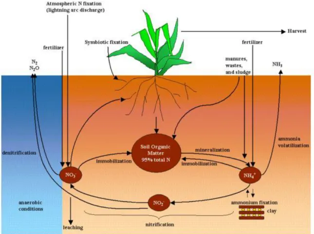
Figure 0.1. The nitrogen cycle. ...2

Figure 0.2. Uranium-238 decay series with Radon...3

Figure 0.3. An illustration of BME methodology. ...7

Figure 1.1. Comparison of LUR-BME results between the monitoring well model and private well model nitrate concentrations. ...28

Figure 1.2. Elasticity curves for monitoring well sources. ...32

Figure S1.1. North Carolina study area with private well and monitoring well nitrate databases ...53

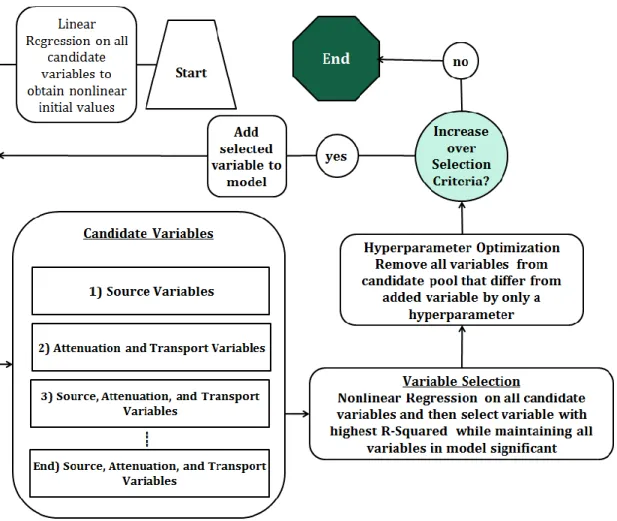
Figure S1.2. Flow diagram of the constrained forward nonlinear and hyperparameter optimization model selection procedure. ...54

Figure S1.3. Histogram of monitoring well data only observed above the detection limit ...55

Figure S1.4. Land Use Regression results from the Constrained Forward Nonlinear Regression and Hyperparameter Optimization procedure for the monitoring and private well models. ...56

Figure S1.5. Monitoring well nitrate LUR residual experimental and modeled spatial and temporal covariance.. ...57

Figure S1.6. Private well nitrate LUR residual experimental and modeled covariance. ...57

Figure S1.7. Level III Ecoregions in North Carolina defined by the US Environmental Protection Agency. ...58

Figure S1.8. Observed monitoring well nitrate from this study overlaid with the GWAVA-SW model results. ...59

Figure S1.9. Observed private well nitrate from this study overlaid with the GWAVA-DW model results. ...60

Figure 2.1. Radon data source spatial distribution detailed by its source. ...67

Figure 2.2. Visualization of elliptical geology based variables. ...70

Figure 2.3. LUR-BME radon predicted median and variance across North Carolina. ...77

(14)

xiv

Figure S2.2. Hibbard 2006 Lithotectonic elements geological descriptions. ...88

Figure S2.3A. Hibbard 2006 Units geological descriptions. ...89

Figure S2.10. Radon LUR residual experimental anisotropic covariance for the Blue Ridge physiographic region.. ...96

Figure S2.13. A rose diagram for radon LUR residual within the Blue Ridge physiographic region. ...99

Figure S3.1. USEPA Indoor Air Radon risk zones by county ...126

Figure S3.2. Pearson residual covariance plots ...127

(15)

1

INTRODUCTION

In order to protect the public from harmful contaminants in the environment, public health scientists conduct risk assessments, which have four basic steps: 1) risk identification, 2) exposure assessment, 3) dose-response characterization, and 4) health-risk characterization. There are many established methods to conduct exposure assessments and to characterize the dose-response relationship between a contaminant of concern and a health outcome; however, many require extensive time and monetary resources that are becoming increasingly limited. Developing geostatistical methods that utilize publicly available data to conduct risk assessment steps not only further develop our understanding of the contaminant of concern and protect public health, but also increase the returns on public resources spent on environmental and public health monitoring.

Understanding the risk of groundwater nitrate (𝑁𝑂₃−) and radon (222𝑅𝑛) exposure is important because they are potential and known human carcinogens, respectively. The three studies in this work address the need for exposure assessment for groundwater 𝑁𝑂₃− and 222𝑅𝑛 and the dose-response characterization for 222𝑅𝑛. The goals of this work are to further develop the spatiotemporal geostatistical methods that can utilize publicly available environmental and human health data, and to apply them to the novel assessment of groundwater 𝑁𝑂₃− and 222𝑅𝑛in North Carolina.

Nitrate Background

(16)

2

cultivated crops, human and animal waste, combustion of fossil fuels including stationary and mobile sources, and other industrial processes.

Figure 0.1. The nitrogen cycle. Figure verbatim from the Soil Water and Assessment Tool theoretical documentation, Neitsch et al. 2009 3.

Exposure to 𝑁𝑂₃− can cause many deleterious health effects in humans. For instance, infants exposed to NO3- can develop methemoglobinemia, or blue baby syndrome4. This adverse endpoint is the basis of the 10 mg/L maximum contaminant level (MCL) in drinking water5. More recent studies have found associations between 𝑁𝑂₃− exposures at levels lower than the current MCL and cancers including colon6, bladder7, and Non-Hodgkin’s Lymphoma8. Ecological effects resulting from excess 𝑁𝑂₃− in the environment include eutrophication of waterways, harmful algal blooms, and fish kills among others 9–11.

Radon Background

(17)

3

Figure 0.2. Uranium-238 decay series with Radon, the radionuclide of interest, highlighted in blue. The top row of each box is the element symbol and isotope number. The second row is the half-life time. Figure modified from Hall et al., 1985. Alpha decay is the release of 2 protons and two neutrons (a helium atom). Beta decay is the release of an electron and a proton changing to a neutron. y refers to years, d to days, m to minutes, and s to second.

222_𝑅𝑛

(18)

4

groundwater used for showering, dishwashing, and clothes washing resulting in exposures in direct vicinity to the breathing zone 19,20.

Land Use Regression

Land use regression (LUR) is a common statistical approach used for exposure

assessments, which was introduced in the EU-funded SAVIAH (Small Area Variations in Air quality and Health) project in 199721. Since LUR was introduced, over a hundred studies implemented LUR to assess exposure of air quality22–24 and water quality contaminants25–28. LUR uses spatially based explanatory variables to model outcomes using classical regression methods. Examples of LUR explanatory variables include land use/land cover (LULC), altitude, river networks, road networks, and point source locations to name just a few. The major benefits of LUR include: 1) Simplicity as a regression-based approach; 2) The plethora of explanatory data sources with the increase of geographic information systems (GIS) and satellite databases; and 3) Physical interpretations of explanatory variables.

A LUR follows a standard regression format as follows:

𝑌𝑖 = 𝛽0+ ∑ 𝛽𝑙𝑋𝑖𝑙 𝐿

𝑙=1

+ 𝜀𝑖 (0.1)

where 𝑌𝑖 is the outcome or dependent variable of interest at data point 𝑖, 𝑋𝑖𝑙 is explanatory or independent variable 𝑙 at point 𝑖, 𝛽_𝑙 is the regression coefficient for variable 𝑋𝑙, 𝛽₀ is the regression equation constant, 𝜀𝑖 is the error term for point 𝑖, and the summation represents the ability to include multiple explanatory variables. The LUR implementation of the regression equation is aided by including a spatial and/or time parameter dependency as follows:

𝑌_𝑖(𝒔, 𝑡) = 𝛽₀+ ∑ 𝛽_𝑙𝑋_𝑖𝑙_{(𝒔, 𝑡)} 𝐿

𝑙=1

+ 𝜀_𝑖 (0.2)

where 𝑌_𝑖(𝒔, 𝑡) is the dependent variable for point 𝑖 at spatial location 𝒔 and temporal location 𝑡, and 𝑋_𝑖𝑙(𝒔, 𝑡) is explanatory variable 𝑙 at point 𝑖 at the same spatial location 𝒔 and temporal location 𝑡. Model coefficients are determined with same techniques available for ordinary linear regression such as ordinary least squares (OLS) and generalized least squares (GLS). In

(19)

5

or with techniques developed specifically for LUR such A Distance Decay Regression Selection Strategy22.

Bayesian Maximum Entropy

Bayesian Maximum Entropy (BME) is a modern spatiotemporal geostatistical framework for incorporating measurements as well as various knowledge bases in a logical and theoretically sound manner to produce estimates of variables of interest at unmonitored locations29. BME therefore is an extremely valuable tool that can be used to produce information of chemical levels and disease rates through space and time by making efficient use of available monitoring resources. BME consists of three epistemological stages known as the prior, meta-prior, and

posterior stages.

It is important to first define the notation and some basic concepts for discussing these BME stages: The notation for a single random variable Z in capital letter, its realization, z, in lower case; and vectors and matrices in bold faces, e.g. 𝒁 = [𝑍₁, … , 𝑍_𝑛]𝑇 and 𝒛 = [𝑧₁, … , 𝑧_𝑛]𝑇. Let 𝜒(𝒑) be the space/time random field (S/TRF) describing the distribution of a variable of interestacross space and time, where 𝒑 = (𝒔, 𝑡), 𝒔 is the space coordinate and 𝑡 is time. The prior stage (Figure I3, Panel A) consists of gathering information or knowledge about the space/time distribution of the variable of interest and compiling it into the general knowledge base,𝐺 − 𝐾𝐵. In the prior stage the 𝐺 − 𝐾𝐵 is mathematically a set of integral equations, which represent constraints on the space/time distribution of 𝝌_𝑚𝑎𝑝:

𝐸[ℊ𝛼] = ∫ 𝑓𝜒(𝝌𝑚𝑎𝑝)𝓰𝜶( 𝝌𝑚𝑎𝑝 )𝑑𝝌𝑚𝑎𝑝 (0.3) where 𝛼 = 0,1, … , 𝑁_𝑐 is the number of suitable constraint functions, 𝑓_𝜒(𝝌_𝑚𝑎𝑝) is the probability distribution function (PDF) of 𝝌𝑚𝑎𝑝 = [𝑥1, … , 𝑥𝑚𝑥𝑘]𝑇, ℊ𝛼(𝝌𝑚𝑎𝑝) are known functions of 𝝌, and 𝐸[. ] is the expected value operator. Functions that describe the space/time distribution include the mean trend, covariance, higher-order moments such as the trivariance, regression equations, and stochastically represented mechanistic equations (i.e. physical laws). The prior PDF describing the space/time distribution of 𝝌_𝑚𝑎𝑝 is given by:

𝑓_𝜒(𝝌_𝑚𝑎𝑝) = exp ( 𝜇₀+ ∑ 𝜇_𝛼ℊ_𝛼(𝜒_𝑚𝑎𝑝) 𝑁𝑐

𝛼=1

(20)

6

where 𝜇_𝛼, (𝛼 = 0,1, … , 𝑁_𝑐) are Lagrange coefficients that are solved for via the system of

𝑁_𝑐+ 1 equations, with the first equation, ∫ 𝑓_𝜒(𝝌_𝑚𝑎𝑝) 𝑑𝝌_𝑚𝑎𝑝 = 1, as the normalization constraint.

In the meta-prior stage one gathers and organizes all of the information that can be explicitly incorporated into BME in the site-specific knowledge base, 𝑆 − 𝐾𝐵. This entails identifying hard data, 𝑆: 𝝌_{ℎ𝑎𝑟𝑑}, or data without measurement error (Figure 0.3, Panel B); soft data, 𝑆: 𝝌_{𝑠𝑜𝑓𝑡}, or data with measurement error that is expressed mathematically as a distribution function. Soft data can be data that has inherent error quantified in its measurements (Figure 0.3, Panel C) or data that is the result of a model prediction with confidence bounds (Figure 0.3, Panel D). An important part of BME is that the soft data can be represented with any distributional form, or is not limited to linear, normal/Gaussian distributions. For example, possible soft data distributions in addition to Gaussian are interval, truncated-Gaussian, or cumulative distribution function. This flexibility in distributions allow for more accurate modeling of environmental contaminants. In practice, the information in the meta-prior stage is often used in the prior stage to empirically derive the functions for the general knowledge base such as the mean trend and covariance.

The posterior stage (Figure 0.3, Panel E) updates the prior PDF, 𝑓_𝜒(𝝌_𝑚𝑎𝑝) , with site-specific knowledge from the meta-prior stage using Bayesian conditionalization, which is essentially the marginal PDF of 𝑓_𝜒(𝝌_𝑚𝑎𝑝) with respect to 𝝌_{𝑠𝑜𝑓𝑡} or 𝝌_{ℎ𝑎𝑟𝑑}, depending on the scenario. Given the scenario of hard data and probabilistic soft data, the BME posterior PDF for a given estimation point 𝑥_𝑘 is given by:

𝑓_𝑘(𝝌_𝒌) = 𝐴−1_{∫ 𝑓}

𝜒(𝒙𝒉𝒂𝒓𝒅, 𝒙𝒔𝒐𝒇𝒕, 𝑥𝑘)𝑓𝜒(𝒙𝒔𝒐𝒇𝒕)𝑑𝝌𝑠𝑜𝑓𝑡

𝐷 (0.5)

where

𝐴 = ∫ 𝑑𝜒𝑘 𝐷

∫ 𝑓𝐺(𝒙𝒔𝒐𝒇𝒕, 𝒙𝒉𝒂𝒓𝒅, 𝑥𝑘)𝑑𝝌𝑠𝑜𝑓𝑡

𝐷 (0.6)

is the normalization constraint, and ∫ (. )_𝐷 is the integral over the domain of the soft data.

When the general knowledge base consists of the mean trend and covariance only and the site-specific data contains only hard data or soft data with a Gaussian measurement error, then BME reduces to the Kriging estimator. As BME currently stands in its numerical

(21)

7

through the mean trend as opposed to additional ℊ_𝛼 functions in the general knowledge base at the prior stage.

(22)

8 Project Themes

The goal of this work is to advance the spatiotemporal geostatistical methods that are utilized in exposure assessments and epidemiological studies; and to demonstrate methodological improvements in the modeling of groundwater 𝑁𝑂₃− and 222𝑅𝑛in North Carolina.

Methodological themes that are present in this work include: 1) Land Use Regression model development for groundwater contaminants; 2) Implementation of space/time BME estimation for groundwater contaminants; 3) Integration of Land Use Regression models into the Bayesian Maximum Entropy framework; 4) Model selection procedures in large variable space problems; 5) Quantitative comparisons of model results arising from differences in spatial scales of

independent and dependent variables; and 6) Quantitative comparisons between the current state of science in exposure estimates and dose-response characterization and the novel developments from this work.

Accurate and precise exposure assessments are important for both nitrate and radon due to their significant human and ecological health risks. Not only is a detailed mapping of

groundwater nitrate important from a biogeochemical perspective31, but it also poses known and potential human health effects, including cancers6,7, that need quality exposure assessments for further study. Similarly, radon has known and potential human carcinogenetic effects. This dissertation addresses that need by providing a framework for more accurate exposure

assessment, which is shown with two case studies of nitrate and radon. Additionally, it will be shown that the exposure assessments can then be utilized in an epidemiological analysis to help elucidate the association between exposures and a response, which in this case is radon and cancers of the stomach and lung. In short, this work comprises two exposure assessments and one dose-response characterization through an epidemiological analysis.

Dissertation Organization

This dissertation is organized into three chapters, with each chapter formatted as a

(23)

9

information pertinent to radon including lithological and uranium data. This manuscript has been submitted to the journal Water. Third, the exposure assessment of groundwater radon is used in the dose-response characterization of groundwater radon to the health outcomes of stomach and lung cancer via an epidemiological analysis at the ecological and the address-level scales. We plan on submitting this manuscript to the journal International Journal of Epidemiology in the near future.

(24)

10

REFERENCES

(1) US Environmental Protection Agency. Basic Information About Nitrate in Drinking Water http://water.epa.gov/drink/contaminants/basicinformation/nitrate.cfm (accessed Nov 1, 2012).

(2) Doering, O. C. I.; Galloway, J. N.; Theis, T. L.; Aneja, V.; Boyer, E.; Cassman, K. G.; Cowling, E. B.; Dickerson, R. R.; Herz, W.; Hey, D. L.; et al. Reactive Nitrogen in the United States: An Analysis of Inputs, Flows, Consequences, and Management Options. EPA-SAB-11-013; Washington D.C., 2011.

(3) Neitsch, S. L.; Arnold, J. G.; Kiniry, J. R.; Williams, J. R. Soil & Water Assessment Tool Theoretical Documentation. 2009.

(4) Comly, H. H. Cyanosis in infants caused by nitrates in well water. J. Am. Med. Assoc.

1945, 129, 112–116.

(5) Spalding, R. F.; Exner, M. E. Occurrence of Nitrate in Groundwater—A Review. J. Environ. Qual. 1993, 22, 392–402.

(6) De Roos, A. J.; Ward, M. H.; Lynch, C. F.; Cantor, K. P. Nitrate in Public Water Supplies and the Risk of Colon and Rectum Cancers. Epidemiology 2003, 14, 640–649.

(7) Weyer, P. J.; Cerhan, J. R.; Kross, B. C.; Hallberg, G. R.; Kantamneni, J.; Breuer, G.; Jones, M. P.; Zheng, W.; Lynch, C. F. Municipal Drinking Water Nitrate Level and Cancer Risk in Older Women : The Iowa Women’s Health Study. Epidemiology 2001, 12, 327–338.

(8) Ward, M. H.; Mark, S. D.; Cantor, K. P.; Weisenburger, D. D.; Correa-Villasenor, A.; Zahm, S. H. Drinking Water Nitrate and the Risk of Non-Hodgkin ’ s Lymphoma.

Epidemiology 1996, 7, 465–471.

(9) Paerl, H. W. Coastal eutrophication and harmful algal blooms : Importance of atmospheric deposition and groundwater as “ new ” nitrogen and other nutrient sources. Limnol.

Oceanogr. 1997, 42, 1154–1165.

(10) Zhou, M.; Shen, Z.; Yu, R. Responses of a coastal phytoplankton community to increased nutrient input from the Changjiang (Yangtze) River. Cont. Shelf Res. 2008, 28, 1483– 1489.

(11) Smith, V. H.; Tilman, G. D.; Nekola, J. C. Eutrophication: impacts of excess nutrient inputs on freshwater, marine, and terrestrial ecosystems. Environ. Pollut. 1999, 100, 179– 196.

(25)

11

(13) Krewski, D.; Lubin, J. H.; Zielinski, J. M.; Alavanja, M.; Catalan, V. S.; Field, R. W.; Klotz, J. B.; Letourneau, E. G.; Lynch, C. F.; Lyon, J. I.; et al. Residential Radon and Risk of Lung Cancer. Epidemiology 2005, 16, 137–145.

(14) Lubin, J. H.; Boice, J. D. Lung cancer risk from residential radon: meta-analysis of eight epidemiologic studies. J. Natl. Cancer Inst. 1997, 89, 49–57.

(15) Field, R. W.; Smith, B.; Steck, D.; Lynch, C. F. Residential radon exposure and lung cancer: variation in risk estimates using alternative exposure scenarios. J. Expo. Anal. Environ. Epidemiol. 2002, 12, 197–203.

(16) Kendall, G. M.; Smith, T. J. Doses to organs and tissues from radon and its decay products. J. Radiol. Prot. 2002, 22, 389–406.

(17) Campbell, T.; Mort, S.; Fong, F.; Crawford-Brown, D.; Vengosh, A.; Cornell, E.; Field, W. R. North Carolina Radon-in-Water Advisory Committee Report; Raleigh, North Carolina, 2011.

(18) National Research Council. Risk Assessment of Radon in Drinking Water; Washington D.C., 1999.

(19) Vinson, D. S.; Campbell, T. R.; Vengosh, A. Radon transfer from groundwater used in showers to indoor air. Appl. Geochemistry 2008, 23, 2676–2685.

(20) Fitzgerald, B.; Hopke, P. K. Experimental Assessment of the Short- and Long-Term Effects of Rn from Domestic Shower Water on the Dose Burden Incurred in Normally Occupied Homes. 1997, 31, 1822–1829.

(21) Briggs, D. J.; Collins, S.; Elliott, P.; Fischer, P.; Kingham, S.; Lebret, E.; Pryl, K.; Van Reeuwijk, H.; Smallbone, K.; Van Der Veen, A. Mapping urban air pollution using GIS: a regression-based approach. Int. J. Geogr. Inf. Sci. 1997, 11, 699–718.

(22) Su, J. G.; Jerrett, M.; Beckerman, B. A distance-decay variable selection strategy for land use regression modeling of ambient air pollution exposures. Sci. Total Environ. 2009, 407, 3890–3898.

(23) Raaschou-Nielsen, O.; Andersen, Z. J.; Beelen, R.; Samoli, E.; Stafoggia, M.; Weinmayr, G.; Hoffmann, B.; Fischer, P.; Nieuwenhuijsen, M. J.; Brunekreef, B.; et al. Air pollution and lung cancer incidence in 17 European cohorts: prospective analyses from the

European Study of Cohorts for Air Pollution Effects (ESCAPE). Lancet. Oncol. 2013, 14, 813–822.

(26)

12

(25) Hoos, A. B.; Mcmahon, G. Spatial analysis of instream nitrogen loads and factors controlling nitrogen delivery to streams in the southeastern United States using spatially referenced regression on watershed attributes ( SPARROW ) and regional classification frameworks. Hydrol. Process. 2009, 23, 2275–2294.

(26) McLay, C. D.; Dragten, R.; Sparling, G.; Selvarajah, N. Predicting groundwater nitrate concentrations in a region of mixed agricultural land use: a comparison of three

approaches. Environ. Pollut. 2001, 115, 191–204.

(27) Aelion, C. M.; Conte, B. C. Susceptibility of residential wells to VOC and nitrate contamination. Environ. Sci. Technol. 2004, 38, 1648–1653.

(28) Messier, K. P.; Akita, Y.; Serre, M. L. Integrating address geocoding, land use regression, and spatiotemporal geostatistical estimation for groundwater tetrachloroethylene. Environ. Sci. Technol. 2012, 46, 2772–2780.

(29) Christakos, G.; Li, X. Bayesian Maximum Entropy Analysis and Mapping : A Farewell to Kriging Estimators ? Math. Geol. 1998, 30, 435–462.

(30) LoBuglio, J. N.; Characklis, G. W.; Serre, M. L. Cost-effective water quality assessment through the integration of monitoring data and modeling results. Water Resour. Res. 2007,

43, 1–16.

(31) Rivett, M. O.; Buss, S. R.; Morgan, P.; Smith, J. W. N.; Bemment, C. D. Nitrate

attenuation in groundwater: a review of biogeochemical controlling processes. Water Res.

(27)

13

CHAPTER 1

Nitrate Variability in Groundwater of North Carolina using Monitoring and Private Well Data Models

Kyle P. Messier†, Evan Kane‡, Rick Bolich‡, Marc L. Serre†*

Authors’ Affiliation:

† Department of Environmental Science and Engineering, Gillings School of Global Public

Health, University of North Carolina, Chapel Hill, NC

‡ North Carolina Department of Environment and Natural Resources, Division of Water Resources

*Corresponding Author: Marc L. Serre

Department of Environmental Sciences and Engineering, Gillings School of Global Public Health, University of North Carolina, 1303 Michael Hooker Research Center, Chapel Hill, NC 27599

(28)

14 Abstract

(29)

15 Introduction

Nitrate (𝑁𝑂₃−) is a widespread contaminant of groundwater and surface water across the United States that has deleterious effects to human and ecological health1,2. The maximum contaminant level of 10 mg/L established by the U.S. Environmental Protection Agency was based on the prevention of methemoglobinemia in infants3; moreover, there is concern of many cancer types 4–6 and from lower concentration exposures7. Excessive 𝑁𝑂₃−inputs into the

environment can result in adverse changes to ecosystems such as eutrophication and harmful algal blooms8–10.

Protection of drinking water sources is mandated by the Safe Drinking Water Act; however, private well drinking water is unregulated in contrast to regulated public water systems11. In North Carolina where more than ¼ of the population relies on private wells for drinking water12, quantifying potential exposures is important to protect public health. Monitoring programs such as the US Geological Survey’s (USGS) National Water Quality Assessment (NAWQA) Program13 and the NC Division of Water Resources (NC DWR) ambient monitoring program14 are effective because they use consistent sampling and analytical methods, yet this water quality monitoring data is spatially and temporally sparse.

Land use regression15–21(LUR) is a proven method that complements monitoring

programs and provides effective means for water quality exposure assessments. Previous studies have related land use characteristics to 𝑁𝑂₃−contamination in surface waters 22–25 and

groundwater. Additionally, regression-based methods have been implemented for estimating loading to surface waters21,23,24. In North Carolina, groundwater discharge to streams (baseflow) accounts for roughly two-thirds of annual streamflow in the Coastal Plains region of North Carolina26 and may be contributing excess nutrient loads in streams27; however, current surface water models do not directly account for this large source of 𝑁𝑂₃−from baseflow.

(30)

16

regression, methods for model selection based on a large candidate variable space include stepwise logistic regression30,31 and regression tree analysis which approximates nonlinear relationships 32,33; still for continuous variable outcomes with nonlinear models, less rigorous methods for model selection have been developed. The number of candidate variables is generally consolidated to a tractable number through expert knowledge or single variable regression, and then various combinations of models are tested until one finds the best model in terms of a validation statistic like 𝑅2 or Akaike Information Criterion (𝐴𝐼𝐶)15,21,24.

The advanced geostatistical method of Bayesian Maximum Entropy (BME) has also been shown to successfully estimate groundwater quality contaminants19,34. An advantage of BME is its ability to quantify spatial and temporal variability which is then used in the estimation process at unmonitored locations. BME, like all geostatistical methods, is data driven and can only provide reliable estimates within the vicinity of measured values. However, BME utilizes Bayesian epistemic knowledge blending to combine multiple sources of data, which has been successfully demonstrated with incorporation of deterministic mean trend functions into BME for groundwater19.

Local spatial and temporal variability have lead previous studies to reduce

𝑁𝑂₃−_{variability with a combination of spatial smoothing and temporal averaging}15,35,36 . For instance, Nolan and Hitt spatially smoothed 𝑁𝑂₃−by taking watershed averages over their study time period, based on watersheds with an average size of approximately 2000 square-kilometers. They not only helped elucidate trends and potential explanatory variables, but they were able to explain a large percentage in the variability of spatially-smoothed 𝑁𝑂₃−with a 𝑟2of 0.80 for shallow aquifer 𝑁𝑂₃−and 0.77 for deep aquifer 𝑁𝑂₃−. However, this advantage of reducing groundwater 𝑁𝑂₃−variance is also a limitation because factors affecting spatially-smoothed and temporally averaged 𝑁𝑂₃−might not affect point-level 𝑁𝑂₃−, and vice-versa. Furthermore, since groundwater 𝑁𝑂₃−contains significant local variability, the need to provide local estimates of its variability naturally follows. Models developed for predicting spatially-smoothed and temporally averaged 𝑁𝑂₃−will likely not be successful in predicting observed, point-level 𝑁𝑂₃−.

The objectives of this study are to: 1) Develop a novel nonlinear regression model for spatial point-level and time-averaged groundwater 𝑁𝑂₃−concentrations in monitoring and private wells of North Carolina, 2) Produce the first space/time estimates of groundwater 𝑁𝑂₃−

(31)

17

and 3) Compare space/time 𝑁𝑂₃− concentration models to the current standard of spatially averaged 𝑁𝑂₃− concentration models Two nonlinear models, whose form is adopted from Nolan and Hitt15 with components that represent 𝑁𝑂₃−sources, attenuation, and transport, are created and selected with a new model selection framework for nonlinear regression models with

correlated explanatory variables. We then integrate the LUR models into the BME framework to model space/time point-level 𝑁𝑂₃−. Results are of interest to agencies that regulate drinking water sources or that monitor health outcomes from ingestion of drinking water. Additionally, the results can provide guidance on factors affecting the point-level variability of groundwater

𝑁𝑂₃−_{and new resources for more accurate management of}_𝑁𝑂

3− loads. Methods

Nitrate Data

𝑁𝑂₃−_{data across North Carolina are obtained from three data sources (Figure S1.1),} which are detailed as follows:

North Carolina Division of Water Resources (NC-DWR) collects data near select permitted, dedicated Wastewater Treatment Residual (WTR) application fields via monitoring wells. The second source is USGS data obtained through the National Water Information System (NWIS). Well depth information is not linked directly to each monitoring well, although a subset of well depth information is available. Based on the subset with depth information, they have a mean depth of 33 feet with a standard deviation of 32 feet. Together, the NCDWR and USGS data represent shallow aquifer monitoring wells (n= 12,322), which hereafter will be referred to as “Monitoring Well data.”

The last dataset of groundwater 𝑁𝑂₃−comes from private well data collected by the North Carolina Department of Health and Human Services (NC-DHHS). Groundwater 𝑁𝑂₃−was obtained and address geocoded using the same process outlined in Messier et al.19. Well depth information is not linked to water quality measurements, but a separate database on private well construction contains well depths. The mean depth is 95 feet with a standard deviation of 109 ft. This data will hereafter be referred to as “Private Well data” and this data is assumed to represent a deeper aquifer model of groundwater 𝑁𝑂₃− (n=22,067).

(32)

18

percent observed above the detection limit is 79.7, 61.4, and 30.6 respectively. Additional basic statistics for the dataset are available in the supporting information (Table S1.1).

Spatial and Temporal Observation Scales

In this work we develop models for 𝑁𝑂₃−at three observation scales. The finer scale corresponds to the space/time point-level𝑁𝑂₃−data, i.e. 𝑁𝑂₃−data as it is sampled. An

intermediate observation scale corresponds to the time-averaged data, whereby 𝑁𝑂₃−at each well is averaged. The time-averaged data provides point-level spatial resolution, but no time

variability. Finally, the coarser resolution observation scale corresponds to the

spatially-smoothed/time-averaged data, which was obtained by spatially smoothing the time-averaged data using a 25 km exponential kernel function. We choose 25 km as it is approximately the average size of watersheds in many NAWQA groundwater studies15,37. While previous works over large study domains have developed models for spatially-smoothed/time average 𝑁𝑂₃−data, very few models, if any, have been developed for point-level 𝑁𝑂₃−data over large study domains. Our work therefore fills that knowledge gap.

Maximum Likelihood Estimation of Nitrate Distributions

Our notation for variables denotes a single random variable Z in capital letter, its realization, z, in lower case; and vectors and matrices in bold faces, e.g. 𝒁 = [𝑍₁, … , 𝑍_𝑛]𝑇 and 𝒛 = [𝑧₁, … , 𝑧_𝑛]𝑇.

Due to the high percentage of nondetect (left-censored) data in both the monitoring well and private well databases, a maximum likelihood estimation (MLE) is used for the estimation of monitoring well and private well distribution parameters38, which is assumed to follow a

lognormal distribution. MLE can directly account for the nondetect values by modifying the likelihood equation, with the censored observations given by the cumulative distribution function (CDF) evaluated at the detection limit. The MLE equation then becomes38:

ℒ(𝒛|𝜇, 𝜎) = { ∏ 𝑓_𝜇,𝜎(𝑧𝑖) 𝑧_𝑖|𝑧_𝑖≥𝑡_𝑖

} ∗ { ∏ 𝐹_𝜇,𝜎(𝑡𝑖) 𝑧_𝑖|𝑧_𝑖≤𝑡_𝑖

} (1.7)

(33)

19

wells and to handle nondetect data. For the regression analysis, the log- 𝑁𝑂₃−concentration of a measurement below detection limit 𝑡_𝑖 is assigned a value equal to the mean of the normal distribution N(𝜇,𝜎) truncated above log(𝑡𝑖), whereas the geostatistical analysis can handle the full truncated normal distribution19.

Spatial Explanatory Variables

Spatial explanatory variables representing possible groundwater 𝑁𝑂₃−sources, attenuation, and transport factors were constructed prior to model development. Potential variables are summarized below with details available in the supporting information (Table S1.2).

All of the explanatory variables have an inherent spatial distance parameter such as circular buffer radius or exponential decay range, which hereinafter is referred to as the

hyperparameter. Each variable is calculated with multiple hyperparameter values since optimal distance is unknown a priori. In the final model selection process, a maximum of one

hyperparameter value is allowed to be selected from each variable to avoid multicollinearity and effectively optimize the hyperparameter. The following variables adopted from Nolan and Hitt15 are 𝑁𝑂₃−sources calculated as Kg − NO₃−/yr/ha within a circular buffer: Sources include farm fertilizer, non-farm fertilizer, manure, and 𝑁𝑂₃−atmospheric deposition. Each National

Landcover Database (NLCD) category is calculated as a percent within a circular buffer. On-site wastewater treatment plant variables, septic density and average nitrate loading, are created following the methods of Pradhan et al.39 The following point sources are calculated as the sum of exponentially decaying contribution19: Wastewater treatment residual field application sites (WTR), swine confined animal feeding operations (CAFOs), poultry CAFOs, cattle farms, and wastewater treatment plants (WWTP). Mean slope in degrees and topographic wetness index40 (TWI) are calculated within circular buffers. Water withdrawals in cubic meters per second are calculated using USGS water use estimates12. Lastly, population density is calculated within circular buffers from US Census block data assuming an even distribution of population per census block.

Nonlinear Regression Model Selection

(34)

20

(SPARROW) 21,23,24. We partition explanatory variables into source, attenuation, and transport terms. Following Nolan and Hitt15, the nonlinear multivariable model is constructed as follows:

z_i = 𝛽₀+ {∑ 𝛽_𝑘𝑌_𝑖(𝑘)(𝜆_𝑘) 𝐾

𝑘=1

} exp {∑ −𝛾_𝑙𝑌_𝑖(𝑙)(𝜆_𝑙) 𝐿

𝑙=1

} exp { ∑ 𝛿_𝑚𝑌_𝑖(𝑚)(𝜆_𝑚) 𝑀

𝑚=1

}

+ 𝜀_𝑖

(1.8)

where zi is the log–transform of 𝑁𝑂3−concentration at point i, 𝛽0 is the intercept, 𝑌_𝑖(𝑘)(𝜆𝑘) is the

k-th source predictor variable at point i with hyperparameter value k, 𝛽𝑘 is its source regression coefficient, 𝑌_𝑖(𝑙)(𝜆𝑙) is the l-th attenuation predictor variable at point i with hyperparameter value 𝜆_𝑙, 𝛾_𝑙is its attenuation regression coefficient, 𝑌_𝑖(𝑚)(𝜆_𝑚)is the m-th transport predictor variable with hyperparameter value 𝜆_𝑚, 𝛿_𝑚 is its transport regression coefficient, and i is an error term. The model contains an additive, linear submodel for sources, and multiplicative exponential terms for the attenuation and transport variables that act directly on the source terms 15. For example 𝑌_𝑖(𝑘)(𝜆_𝑘) may be equal to a land cover variable or a point source variable. The

attenuation variables,𝑌_𝑖(𝑙), physically represent areas that are associated with removing 𝑁𝑂₃−from groundwater such as wetlands and histosol soil. The transport variables, 𝑌_𝑖(𝑚)(𝜆_𝑚), may be equal to any variable that effects the movement of 𝑁𝑂₃−in the groundwater such as the soil

permeability and average slope. The attenuation variable coefficients,𝛾_𝑙, are constrained to be negative allowing them to only decrease 𝑁𝑂₃− concentrations, while the transport variable coefficients,𝛿_𝑚, are unconstrained allowing variables to increase or decrease

𝑁𝑂₃−_{concentrations.}

We developed a nonlinear model regression model selection technique that

accommodates variables that differ only by a hyperparameter and can be adapted for various nonlinear model forms. Our model selection procedure is essentially a nonlinear extension of A Distance Decay REgression Selection Strategy (ADDRESS)16, since to the authors’ knowledge there is not a regression selection strategy for nonlinear LUR. We implement Constrained Forward Nonlinear Regression with Hyperparameter Optimization (CFN-RHO) whose simple algorithm is as follows (Figure S1.2):

(35)

21

2) Candidate Variables: In the first iteration, the candidate variables consist of the source variables only. In the second iteration, candidate variables consist of attenuation and transport variables only. This is done so as to obtain an initial model with at least one source and one attenuation or transport variable. In every iteration afterwards the candidate variables can be any variable.

3) Nonlinear Regression: Nonlinear regression is performed by adding each candidate variable to the current model one at a time. Note that candidate variables are added according to their

predetermined place in the nonlinear model (i.e. Source variables are in a linear submodel; Attenuation and transport in the exponential submodel.).

4) Variable Selection: The variable that results in the highest R-Squared (lowest AIC is also an option) while constrained to maintaining all variables in the model statistically significant (p-value < 0.05), is selected and added to the model. R-Squared ties beyond the thousandth decimal place are settled by the lowest p-value.

5) Hyperparameter Optimization: The rest of the candidate variables that differ from the selected variable by only a hyperparameter are removed from the candidate variable pool, effectively optimizing the hyperparameter value.

6) Selection Criteria: The new model must increase R-Squared over user-defined selection criteria such as a one percent increase. If the model passes the selection criteria, then the iterative process continues to step 2. If it does not, then the algorithm ends with the final model being the i-th minus one model since the last variable did not pass the selection criteria.

BME Estimation Framework for Space/Time Mapping Analysis

(36)

22

Let 𝑍(𝒑)be the space/time random field (S/TRF) describing the distribution of

groundwater log- 𝑁𝑂₃−across space and time, where 𝒑 = (𝒔, 𝑡), 𝒔 is the space coordinate and 𝑡 is time. The knowledge available is organized in the general knowledge base (G-KB) about the space/time trend and variability (e.g. mean, covariance) of 𝑁𝑂₃−across the study domain, and the site-specific knowledge base (S-KB) corresponding to the hard and soft data 𝒛_𝒅 available at a set of specific space/time points 𝒑_𝑑.

First, we define the transformation of log- 𝑁𝑂₃−data 𝒛𝒅at locations 𝒑𝒅 as

𝒙𝒉 = 𝒛𝒉− 𝑜𝑍(𝒑𝒉) (1.9)

where 𝑜_𝑍(𝒑_𝒉) may be any deterministic offset that can be mathematically calculated at any space/time coordinate 𝒑. We then define 𝑋(𝒑) as a homogeneous/stationary S/TRF representing the variability and uncertainty with the transformed data 𝒙_𝒅, i.e. such that 𝒙_𝒅 is a realization of

𝑋(𝒑). Finally we let 𝑍(𝒑) = 𝑋(𝒑) + 𝑜_𝑧(𝒑) be the S/TRF representing groundwater log- 𝑁𝑂₃−. In this study, we consider two choices for 𝑜𝑧(𝒑): (1) a constant value determined by the MLE mean resulting in a purely BME model, and (2) the LUR estimate 𝑳_𝒛(𝒑_𝒉) from CFN-RHO resulting in a LUR-BME model.

The G-KB for the S/TRF 𝑋(𝒑) describes its local space/time trends and dependencies. In this work, the general knowledge consists of the space/time mean trend function 𝑚𝑥(𝒑) = 𝐸[𝑋(𝒑)], and the covariance function 𝐶_𝑋(𝒑, 𝒑′)=𝐸[[𝑋(𝒑) − 𝑚_𝑥(𝒑)][X(𝐩′) − 𝑚_𝒙(𝒑′)]] of the S/TRF 𝑋(𝒑). The S-KB consists of hard data and soft data; with hard data, 𝒙_𝒉= 𝒛_𝒉− 𝑳_𝒛(𝒑_𝒉), for data points where 𝒛𝒉 is observed over the detection limit and soft data, 𝑿𝒔, is at locations 𝒑_𝒔where 𝑁𝑂₃−is observed below the detection limit. Following Messier et al 19, the BME soft data for log- 𝑁𝑂₃−is modeled as a Gaussian distribution truncated above the log of the detection limit.

The overall knowledge bases considered consist of 𝐺 = {𝑚𝑥(𝒑), 𝐶𝑋(𝒑, 𝒑′)}, and 𝑆 = {𝑓𝑠(. ), 𝑿𝒉}. In this case the BME set of equations reduces to

𝑓𝐾(𝑥𝑘) = 𝐴−1∫ 𝑑𝒙𝒔𝑓𝐺(𝒙𝒉, 𝒙𝒔, 𝑥𝑘)𝑓𝑆(𝒙𝒔) (1.10 ) where 𝑓_𝐾(𝑥_𝑘) is the BME posterior PDF for the offset-removed log 𝑁𝑂₃−(𝑥_𝑘) at some

(37)

23

Gaussian PDF of 𝑿_𝒔, and 𝐴−1is a normalization constant. After the BME analysis is conducted,

𝑜_𝑍(𝒑) is added back to obtain log- 𝑁𝑂₃−concentrations. Validation Statistics

The robustness of CFN-RHO is tested with a fold cross-validation procedure. In 10-fold cross-validation data is randomly partitioned into 10 equal size subsamples. A single subsample is retained as the validation data for testing the model, and the remaining 9

subsamples are used as training data. Each of the 10 subsamples is used exactly once as the validation data. Similar variable selections (which may differ only by hyperparameter) for subsamples demonstrate model selection robustness.

Models are compared with a leave one-out cross-validation (LOOCV) mean squared error (MSE) and R-Squared. Spatially-smoothed/time-averaged 𝑁𝑂₃− and time-averaged 𝑁𝑂₃− models are also tested on how well they predict at the smaller observation scales. In LOOCV, each

𝑁𝑂₃−_value_𝑍

𝑗 is removed one at a time, and re-estimated using the given model based only on the remaining data. Let 𝑍∗(𝑘)be the re- estimate for method k, then 𝑀𝑆𝐸(𝑘)=_𝑛1∑𝑛_𝑗=1(𝑍_𝑗∗(𝑘)−

𝑍𝑗) 2

and the cross-validation R-Squared is 𝑅2(𝒁, 𝒁∗(𝑘)). Results

Nitrate Concentrations

The MLE of the statewide monitoring concentrations resulted in a geometric mean and standard deviation of the lognormal distribution of 0.62 and 14 mg/L, respectively (Figure S1.3). MLE for private wells resulted in a geometric mean and standard deviation of 0.45 and 5.1 mg/L (Figure S1.3).

Spatially-smoothed/Time-averaged Nitrate

(38)

24

10-fold cross-validation of spatially-smoothed/time-averaged 𝑁𝑂₃− LUR models was done to demonstrate the stability of CFN-RHO (Table S1.4, S1.5). All variables were selected 7 and 10 out of 10 iterations for the monitoring and private well models, respectively.

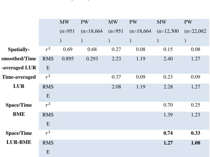
Table 1.1. Leave-one-out cross-validation statistics comparing for four estimation methods that predict spatial/temporally averaged 𝑵𝑶_𝟑−concentrations, temporal averaged 𝑵𝑶_𝟑−concentrations, and point-level observed 𝑵𝑶_𝟑−concentrations. Note that methods were used to predict at scales more refined or equal to its calibration scale. MW = Monitoring Well model. PW= Private Well model. n = number of observations at that scale. Time averaging results in fewer observations. RMSE = Root Mean Squared Error. Units of 𝑵𝑶_𝟑− concentration = mg/L.

Predicted Value

Method

Spatially- smoothed/Time-averaged 𝑁𝑂₃−

Time-averaged

𝑁𝑂₃−

Point-Level 𝑁𝑂₃−

MW (n=951 ) PW (n=18,664 ) MW (n=951 ) PW (n=18,664 ) MW (n=12,300 ) PW (n=22,062 ) Spatially-smoothed/Time -averaged LUR

𝑟2 _0.69 _0.68 _0.27 _0.08 _0.15 _0.08

RMS E

0.895 0.293 2.23 1.19 2.40 1.27

Time-averaged LUR

𝑟2 _0.37 _0.09 _0.23 _0.09

RMS E

2.08 1.19 2.28 1.27

Space/Time BME

𝑟2 _0.70 _0.25

RMS E

1.39 1.23

Space/Time LUR-BME

𝑟2 _0.74 _0.33

RMS E

(39)

25 Time-averaged Nitrate

The LUR variables selected through CFN-RHO for time-averaged 𝑁𝑂₃−observed at monitoring wells and private wells are shown in Table 1.2. The LUR calibrated to predict time-averaged 𝑁𝑂₃−obtains a 𝑟2 of 0.37 and 0.09 for monitoring wells and private wells, respectively (Table 1.1, second row). Moreover, the LUR model predicts point-level 𝑁𝑂₃−with a 𝑟2 of 0.23 and 0.09 for monitoring and private well respectively. LUR maps are available in supporting information (Figure S1.4).

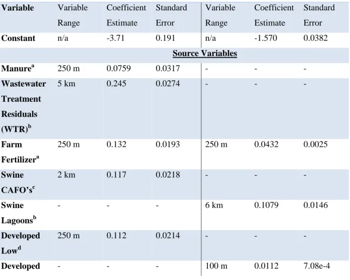
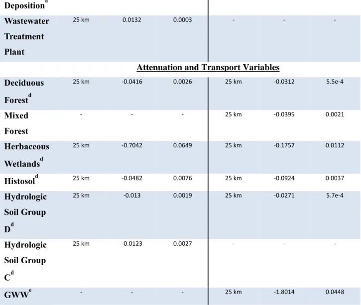
Table 1.2. Nonlinear regression model variables selected via CFN-RHO and parameter estimates for time-averaged 𝑵𝑶_𝟑− monitoring (left) and private well (right) models. All variables are significant with p-value < 0.025. Variables units: a- Kg- 𝑵𝑶_𝟑−/yr/ha, b- Dimensionless, c- 100 pigs, d- percent, e- degrees (-) Not a variable in the model.

Monitoring Well Private Well

Variable Variable Range Coefficient Estimate Standard Error Variable Range Coefficient Estimate Standard Error

Constant n/a -3.71 0.191 n/a -1.570 0.0382

Source Variables

Manurea 250 m 0.0759 0.0317 - - -

Wastewater Treatment Residuals (WTR)b

5 km 0.245 0.0274 - - -

Farm Fertilizera

250 m 0.132 0.0193 250 m 0.0432 0.0025

Swine CAFO’sc

2 km 0.117 0.0218 - - -

Swine Lagoonsb

- - - 6 km 0.1079 0.0146

Developed Lowd

250 m 0.112 0.0214 - - -

(40)

26 (All

combined)d Atmospheric Depositiona

250 m 0.477 0.129 25 km 2.94e-11 2.53e-10

Attenuation and Transport Variables Forest (All

combined)d

2 km -0.0064 0.00281 - - -

Deciduous Forestd

- - - 4 km -0.0151 0.00127

Herbaceous Wetlandsd

5 km -0.531 0.079 - - -

Histosold 25 km -0.0427 0.0111 25 km -0.106 0.0126

Hydrologic Soil Group Dd

- - - 500 m -0.012 0.0010

Slopee 25 km -0.074 0.0261 - - -

10-fold cross-validation of time-averaged 𝑁𝑂₃− LUR models was conducted (Table S1.6, S1.7). All variables selected from the monitoring well model are selected in at least 6 iterations of the ten-fold cross-validation runs. The majority of variables in the private well model were also stable; however swine lagoons and deciduous forest were only selected 2 and 0 out of 10 times. In both models, when a variable is not selected in the 10-fold cross validation it is likely due to other variables that capture similar source, attenuation, or transport processes (i.e. Forest instead of Deciduous, Swine CAFO’s instead of Swine Lagoons).

Point-Level Nitrate

We modeled the space/time covariance of the LUR offset removed log- 𝑁𝑂₃− S/TRF,

𝑋(𝒑), using a two-component, space/time non-separable, exponential covariance model following Messier et al19:

𝐶_𝑋(𝑟, 𝜏) = 𝑐₁exp (−3𝑟

𝑎_𝑟₁) exp (− 3𝜏

𝑎_𝜏₁) + 𝑐2exp (− 3𝑟

𝑎_𝑟₂) exp (− 3𝜏 𝑎_𝜏₂)

(41)

27

where 𝑐₁ = 0.67 (𝑙𝑜𝑔 − 𝑚𝑔/𝐿)2 , 𝑎_𝑟₁ = 93 𝑚 ,𝑎_𝜏₁ = 15 𝑑𝑎𝑦𝑠, 𝑐₂ = 3.6 (𝑚𝑔/𝐿)2, 𝑎_𝑟₂ =

1750 𝑚, 𝑎_𝜏₂ = 15840 𝑑𝑎𝑦𝑠 for monitoring wells (Figure S1.5) and a one-component, space/time exponential covariance model for private well where 𝑐1= 0.76 (𝑙𝑜𝑔 − 𝑚𝑔/𝐿)2 , 𝑎𝑟1 = 1181 𝑚 ,𝑎𝜏1 = 8640 𝑑𝑎𝑦𝑠 (Figure S1.6).

(42)

28

(43)

29 Discussion

Groundwater Nitrate Maps

This study presents a LUR model for point-level 𝑁𝑂₃−in North Carolina that elucidates processes affecting its local variability, and then utilizes the strengths of BME to create the first LUR-BME model of groundwater nitrate’s spatial/temporal distribution including prediction uncertainty. The first major finding is the LUR-BME model for monitoring wells, assumed to represent surficial aquifers, (Figure 1.1, Movie S1) shows groundwater 𝑁𝑂₃−that is highly variable with many areas predicted above the current standard of 10 mg/L.

Contrarily, the private well results (Figure 1.1) depict widespread, low-level 𝑁𝑂₃−

concentrations, which is consistent with the current physical understanding in which sources tend to pollute the surficial aquifer, but then transport over time to the deeper drinking-water supply aquifers where concentrations are lower. This finding is significant because of the studies demonstrating potential significant health effects at concentrations as low as 2.5 mg/L4–7. Additionally, concentrations of 𝑁𝑂₃−could impact ecological function since there are potential large reserves in deeper aquifers that can discharge to surface waters.27. The standard deviation maps (Figure 1.1) demonstrate the importance of NC-DWR and USGS monitoring wells and private well testing because areas within the spatial covariance range are well characterized, whereas those outside are less reliable.

The second major finding is the LUR-BME maps (Figure 1.1) show that groundwater

𝑁𝑂₃−_{in monitoring wells is elevated in the southeastern plains of North Carolina (Figure S1.7)} due to the larger amount of 𝑁𝑂₃−sources and the lack of subsurface attenuation factors (Movie S2) that are present in the coastal plain region. This corroborates the findings of Nolan and Hitt15, which also show spatially-smoothed/time-averaged 𝑁𝑂₃−to be the highest in the

southeastern plains of North Carolina. This expands that finding with point-level results showing significant point-level variability within regional trends. Additional concerns arise since

groundwater flow of the southeastern plains contributes significantly to surface water flow27. Our LUR-BME model can be used with surface water models to quantify the effect of groundwater

𝑁𝑂₃−_{contributing to surface water contamination.}

(44)

30

significantly less training data and averaging 𝑁𝑂₃−over watersheds. Our LUR-BME models benefit from the large amount of monitoring (n=12,322) and private well (n=22,067) data, whereas they used 2,306 and 2,490 across the US for their shallow and drinking water models, respectively.

LUR-BME benefits from the exactitude property of BME, thus our model results are in 100% agreement at monitoring locations. Contrarily, when our observed data is compared with Nolan and Hitt15 by grouping results according to the bins of figure 1.1, Nolan and Hitt15 over-predicts 48% and 59% of the time for monitoring and private wells, respectively (Figure S1.8,S1.9). As a result of the finer resolution of our maps and their improved ability to predict low level 𝑁𝑂₃−, our results lead to a significant new finding about the extent of areas with low level contamination. Our results show private well concentrations are greater than 0.25 mg/L while monitoring well concentrations are less than 0.25 mg/L in 30.6 percent of North Carolina’s area, compared to 2.6 percent for Nolan and Hitt15 (Table S1.8,S1.9). Likewise, our results show monitoring and private wells are both above or below 0.25 mg/L at the same location in 68 percent of North Carolina, compared to 91 percent for Nolan and Hitt15. Hence whereas Nolan and Hitt15 results suggest the geographical extent of the low level contamination of drinking water aquifer is limited to that of the shallow aquifer, which is consistent with downward transport of 𝑁𝑂₃−contamination, our LUR-BME models shows that in fact the geographical extent of the contamination of the drinking water extends over a much larger area than that of the shallow aquifer. This major new finding provides new evidence indicating that in addition to downward transport, there is also a significant outward transport of groundwater 𝑁𝑂₃−in the drinking water aquifer to areas outside the range of sources. This is especially significant because it indicates that the deeper aquifers are acting as a reservoir that is not only deeper, but also wider than the reservoir formed by the shallow aquifers.

LUR Variable Interpretations

(45)

31

geometric mean of 𝑁𝑂₃−in mg/L for every 1 kg/yr/ha of farm fertilizer is exp(0. 132 ∗ 0.456) =

1.06 = 5% where 0.456 is the exponential of the mean attenuation and transport variables multiplied by their coefficients. For the private well model, the percent increase in the geometric mean of 𝑁𝑂₃−for every 1 kg/yr/ha of farm fertilizer is exp(0.0432 ∗ 0.4636) = 1.02 = 2%. Every other source coefficient interpretation for time-averaged 𝑁𝑂₃−is provided in the supporting information.

Comparing variables selected between the spatially-smoothed/time-averaged 𝑁𝑂₃−LUR and the time-averaged 𝑁𝑂₃− LUR help elucidate effects the spatial scale has on groundwater

𝑁𝑂₃−_{concentrations. The variable hyperparameters selected by CFN-RHO help elucidate} potential scales at which the variables affect groundwater 𝑁𝑂₃−concentrations. For example, the short buffer range of developed low likely captures the small size of single-family housing yards and their associated fertilizer applications. The monitoring well model WTR has an exponential decay range of 5 km. A possible explanation of this medium range is due to the volatization of

𝑁𝑂₃−_{into the air, which can then be transported over longer distances than subsurface transport} mechanisms alone. Long buffer ranges for attenuation and transport variables such as percent histosol soil and mean slope represent variables with larger, regional scale effects.

(46)

32

Figure 1.5. Elasticity curves for monitoring well sources. Y-axis is the percent decrease in a source and the X-axis is the percent decrease in geometric mean, for (A) State-Wide, (B) Within 1-km of Wastewater Treatment Residuals, and (C) Within 1-km of swine CAFO’s.

Recommendations and Limitations

This work represents the first step in the development of modeling observed 𝑁𝑂₃−over large domains without averaging. In previous studies, spatial averaging is utilized because it provides results at the domain (State, Regional, or National) desired for policy making decisions and sheds light on processes influencing groundwater 𝑁𝑂₃−. We demonstrated that a LUR at the point-level in space is currently limited in terms of model predictive capability but when

(47)

33

covariance range similar to LUR models for spatially-smoothed/time-averaged groundwater

𝑁𝑂₃−_{concentrations. Potential explanatory variables that can explain the remaining variability in} the point-level LUR will need primary data collection. For instance, we found WTR to be a significant variable even though we just used location of fields. If records of timing and amounts of WTR applications were improved, then the temporal variability in monitoring wells near WTR application fields could be improved44. Similarly, a parcel-level query of farm fertilizer application practices could distinguish farms that use 𝑁𝑂₃−fertilizers efficiently versus farms that apply excessively or with poor timing. For private wells, the short spatial auto-correlation range may be due to differences in effectiveness of on-site wastewater treatment systems or residential fertilizer use. Additionally, we note that candidate variables not selected via CFN-RHO does not necessarily indicate they have no effect on groundwater 𝑁𝑂₃−concentrations in surficial or confined drinking-water aquifers of North Carolina. Many factors both statistically and physically can affect the selection such as correlation between candidate variables and local hydrogeology conditions being overwhelmed by larger scale trends. This study lacked well depth for the majority of monitoring and private wells. The monitoring and private well models clearly demonstrate a difference in concentrations based on depth, so well depth could quantify this more explicitly as opposed to categorically as done by this study. Furthermore, pumping rate information was not available for the private well data set thus the effect of local pumping could not be quantified. The USGS water use report12 has information on domestic-use water

(48)

34

In conclusion, a LUR model with a novel model selection procedure can elucidate important predictors of point-level groundwater 𝑁𝑂₃−in North Carolina monitoring and private wells. The methods are translatable to other study areas in the United States. LUR-BME models can be used to predict spatial/temporal varying groundwater 𝑁𝑂₃−and provide uncertainty assessments. Further research should integrate groundwater 𝑁𝑂₃−results into surface water models to determine the extent of groundwater’s contribution to surface water contamination. Lastly, results will be useful in identifying localities of elevated 𝑁𝑂₃− for increased monitoring. Acknowledgements

This research was supported in part by funds from the NIH T32ES007018,

NIOSH 2T42OH008673, and North Carolina Water Resources Research Institute (WRRI) project number 11-05-W.

Associated Content