POLITICAL
LOBBYING
W
ITHPRIVATE
INFORMATION
Justin Contat
A dissertation submitted to the faculty of the University of North Carolina at Chapel Hill in par-tial fulfillment of the requirements for the degree of Doctor of Philosophy in the Department of
Economics.
Chapel Hill 2015
Approved by: Sergio Parreiras Gary Biglaiser Fei Li
c
2015 Justin Contat
ABSTRACT
JUSTIN CONTAT: Political Lobbying With Private Information. (Under the direction of Sergio Parreiras)
ACKNOWLEDGMENTS
TABLE OF CONTENTS
LIST OF FIGURES . . . viii
1 Summary . . . 1
1.1 Introduction . . . 1
2 Equilibrium Convergence in the All-Pay Auction . . . 4
2.1 Introduction . . . 4
2.2 Model . . . 6
2.2.1 Information Structure . . . 6
2.2.2 Payoffs . . . 8
2.2.3 Equilibrium Characterization . . . 10
2.3 Convergence of Equilibria . . . 13
2.3.1 Symmetric Convergence of Equilibria . . . 14
2.3.2 Asymmetric Convergence of Equilibria . . . 16
2.4 Conclusion . . . 19
3 Comparative Statics in the All-Pay Auction . . . 20
3.1 Introduction . . . 20
3.2 Complete Information Comparative Statics . . . 23
3.2.1 Symmetric Equilibrium Benchmark . . . 23
3.2.2 The Assimilation Effect: A First Look . . . 23
3.3 Private Information Comparative Statics (Valuations) . . . 26
3.3.2 Symmetric Equilibrium Benchmark . . . 28
3.3.3 Asymmetric Equilibrium: The Assimilation and Stacking Effects . . . 28
3.4 Private Information Comparative Statics (Probabilities) . . . 43
3.4.1 Two Types . . . 44
3.4.2 Three Types . . . 47
3.4.3 Summary of Changing Probabilities . . . 49
3.5 Conclusion . . . 49
4 Maximum Contribution Limits . . . 51
4.1 Introduction . . . 51
4.2 Model and Equilibrium Characterization without Contribution Limits . . . 53
4.3 Maximum Limits with Complete Information . . . 56
4.4 Maximum Limits with Private Information . . . 60
4.4.1 Symmetric Lobbyists . . . 60
4.4.2 Asymmetric Lobbyists . . . 68
4.5 Conclusion . . . 76
LIST OF FIGURES
2.1 Finite-Type Space Distribution . . . 8
2.2 Concavity ofUi(a|µj,n, ti) . . . 12
2.3 Concavity ofσi(ai|·) . . . 13
2.4 Convergence of Equilibrium Supports . . . 14
3.1 Complete Information Equilibrium and Revenues . . . 26
3.2 ∆Rev: p1,1 =p1−andp1,3 =p3+ . . . 48
4.1 Complete Information Equilibrium,C =∞ . . . 57
4.2 Che and Gale (1998)’s Complete Information Revenues . . . 58
4.3 Expected Contributions for Symmetric Lobbyists . . . 68
CHAPTER 1 SUMMARY
1.1 Introduction
In the past decades there has been growing concern about the influence of money in politics. Most recently in 2010, The Supreme Court of the United States of America ruled in Citizens United vs. Federal Elections Commissionthat as long as contributions are made to an independent third party (such as a Super PAC) that the contributions are expressions of free speech and thus protected by the First Amendment to the Constitution of the United States of America. Thus in certain circumstances, individuals are allowed to contribute unlimited amounts of money as long as the contribution is not direct. The main goal of this dissertation is to understand the impact of maximum contribution limits on the behavior of lobbyists relative to a lobbying environment without contribution limits.
I show that the combined effects of private information and asymmetry between lobbyists are needed to fully understand changes in lobbying behavior and total contributions when contribution limits are enacted. Lobbyists have private information about the value of political favor. Each lobbyist does not exactly know the valuation of the other lobbyist, only the relative likelihoods of different valuations (i.e. the probability distribution of valuations). The lobbyists may differ in the relative likelihoods they place on each other’s valuations. In other words, they are ex-ante asymmetric because their type space and type space distributions may differ. Relaxing either pri-vate information or asymmetry between the lobbyists will lead to different qualitative conclusions regarding lobbying behavior.
The first chapter of this dissertation provides a technical result that justifies the use of finite types in the lobbying game. With types drawn from an absolutely continuous distribution, equilibrium behavior is characterized as a solution to system of non-linear first-order differential equations. In all but the simplest distributions, an analytical solution is not possible. In contrast, equilibria under finite types are much easier to describe. The main result of the first chapter is to show that the equilibrium correspondence (in fact it is a function) is continuous with respect to the information structure. Small changes in the type space distribution lead to small changes in equilibrium be-havior. While this result is known to hold in games with continuous payoff functions, the all-pay auction has payoff functions that are neither upper-semicontinuous nor lower-semicontinuous and so that standard results do not apply. The key driver of the results is the monotonicity of the all-pay auction: higher types contribute more with certainty.
The second chapter provides another technical result. It demonstrates the complexity that arises when even a small amount of asymmetry is introduced into the game. In particular, total contri-butions can increase or decrease depending upon how a lobbyist is made stronger relative to the other. Nevertheless we provide conditions under which asymmetry will increase total contribu-tions. Two effects capture the intuition of the results. The first effect, the assimilation effect , shows that lobbyists always play to the level of their competition. Weaker competition means less contributions while stronger competition means more contributions. The second effect, the stack-ing effect, exploits the monotonicity of the lobbystack-ing game. Whenever a type of a lobbyist would want to contribute more, so too must all of the lobbyists higher types. Monotonicity is the most important property of the lobbying game.
CHAPTER 2
EQUILIBRIUM CONVERGENCE IN THE ALL-PAY AUCTION
2.1 Introduction
In an all-pay auction (APA), each player chooses a costly action for a chance to win an indivisible prize. The player with the largest action wins the prize, but allplayers must pay a cost equal to their own action irrespective of who wins. Payments1are totally unconditional in that each player’s
payment does not depend on the actions of others or the allocation of the prize. In this paper I restrict attention to the standard2all-pay auction with two players.
My main result shows that despite the inherent payoff discontinuities in the APA, the equilib-rium correspondence is continuous3 with respect the information structure of the game. In fact,
since each information structure generates a unique equilibrium it would be more appropriate to use the terminology “equilibrium function” instead of equilibrium correspondence. I show that as a sequence of finite type space distributions converge to a continuous distribution, then the sequence of unique equilibria in the finite games converge to the unique equilibrium of the continous-type game. This implies the equilibrium correspondence is both upper and lower hemi-continuous4. In particular, the main result implies that any equilibrium in a continuous-type APA can be approx-imated with an equilibrium of a finite-type APA, provided the type space distributions of the two
1Payments can also be interpreted as costs of acquiring effort, political donations, or investment in R&D for
example. See Konrad (2009) for a more detailed introduction to the theory and application of APA’s.
2In this dissertation the standard all-pay auction means risk neutral players with independent private values.
3It is possible to assign a metric to measure the distance between two probability distributions. The notion of
continuity here would then correspond to the usual−δdefinition, where distance between two distributions is given by the information metric (such as the Levy-Prokhorov metric). See Shiryaev (1996) Chapter III Section 7 for a detailed definition.
4A correspondenceΓ :X
games are close. The mixed strategy equilibria of the finite-type game converge to the pure strategy equilibria of the continuous-type game as the type space becomes finer.
With complete information it is straightforward to show that APA equilibria converge as the valuations converge. In this sense we can say that the equilibrium correspondence is upper hemi-continuous in the information structure when there is complete information. The equilibrium cor-respondence is also trivially lower hemi-continuous. This chapter extends both of these results to the incomplete information APA in a very natural way. Siegel (2013) has the closest result to ours. He shows that for any sequence of distributions for player 1 there existsomesequence of distribu-tions for player 2 such that the sequence of equilibria converge to that of the continuum game. In contrast I show that anysequence of equilibria converge provided their distributions converge as well.
In general it is not true that the Nash equilibrium correspondence is continuous (i.e. both lower and upper hemi-continuous), even for games of complete information. Engl (1995) shows that the equilibrium correspondence is in general not lower hemi-continuous, but is asymptotically lower hemi-continuous in that an equilibrium in the limit game can be approached by a sequence ofn
equilibria. Milgrom and Weber (1985) show upper hemi-continuity of the equilibrium correspon-dence in a class of games with uncountable state spaces, though their results require uniformly continuous payoffs for all players, a condition which is not satisfied by the APA. Additionally they provide an example to show that in general continuity cannot be dropped.
distribution over actions and types that agrees5 with the player’s type-space distribution.
This result complements the literature on equilibrium convergence in the APA. While others have focused on equilibria change as a finite action set is enlarged to that of the continuum, I study how equilibria change as a finitetypeset is enlarged. For a class of games which includes the complete information APA, Dasgupta and Maskin (1986) show that the limit of equilibria, as action sets become finer, is the equilibria of the limit. Similarly Athey (2001) shows that in a class of incomplete information games with certain monotonicity properties6(which includes the APA), equilibria in finite-action games converge to equilibria in continuous-action games when the action sets are made finer and finer and the type space is held fixed. My results, like those of Athey (2001), crucially depend upon the underlying monotonicity of the game.
Amann and Leininger (1996) have shown for continuum types and 2 players that the if the type spaces converge to a single point (i.e. complete information APA) then the associated sequence of equilibria converge as well. This paper complements theirs in that I show that for type spaces “in between” continuum types and a single type (i.e. complete information) the sequence of equilibria converge as well.
2.2 Model
2.2.1 Information Structure
There are two risk-neutral players who compete for a chance to win an indivisible prize worth ti > 0 to playeri. We restrict attention to strictly positive valuations, but this is without loss of
generality because all zero-valuation types will not participate in equilibrium and hence will not affect any of the results. Eachti ∈ Ti,n ≡ {t1i,n, t2i,n, . . . , tmi,n} ⊂ R++is private information and
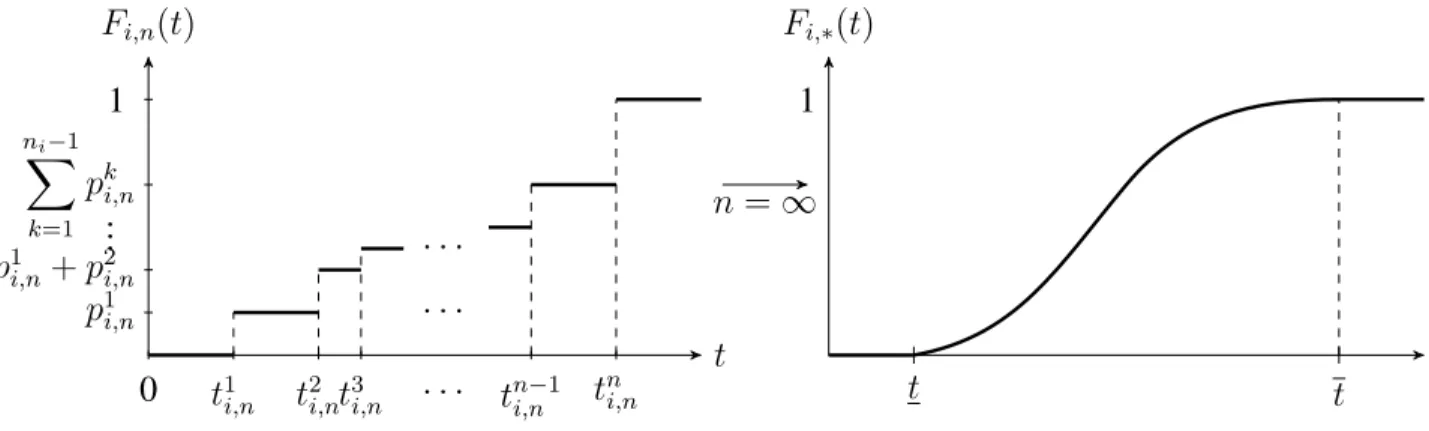
independently distributed according to c.d.f.Fi,n. A typical finite-type distribution is shown on the
left in Figure 2.1. Letpk
i,n≡Fi,n(tki,n)−Fi,n(tki,n−1)denote the probability thatiwill have valuation
tk
i,n. Hence eachFi,n(·)is an increasing piece-wise constant function (i.e. a step function) that is
5The marginal on the distributional strategy must be equal to the probability distribution of type space.
6Her Single Crossing Condition (SCC) states that each player’s best response is increasing in type whenever his
discontinuous on Ti,n, a countable set. There will also be a limiting space Ti,∞ = limn→∞Ti,n,
described in detail in the next paragraph, which we will assume exists. This limiting spaceTi,∞
will be dense in some interval of strictly positive typesTi,∗ ≡[vi, vi]. Hence the sequences ofTi,n
will converge and form a countable dense subset of some closed intervalTi,∗.
Consider any sequence of finite-type c.d.f.’s {Fi,n}n that converges in distribution7 to an
ab-solutely continuous8 distribution F
i,∗ as in Figure 1. In general, each new term in the sequence
{Fi,n}n of finite-type c.d.f.’s may have more or fewer types, where types may be the same or
different. For example it could be the case that Ti,n = {1,2,3,4,5}, Ti,n+1 = {2.1,4.8}, and
Ti,n+2 = {2,2.1,3,4,4.8,5,7}. In addition, the probability of each type typically changes for
ev-ery term in the sequence. Since I am interested in converging sequences of type spaces and their distributions, I will assume that |Ti,n| = n for notational convenience9. We require the limiting
c.d.f. Fi,∗ to represent a continuous distribution. Though my result holds for any sequence of
dis-tributions, in particular we can think of adding types to a finite-type space, where at each iteration after a new type is added the probabilities are adjusted to make the new distribution closer toFi,∗.
In this way continuous-type spaces (i.e. those with absolutely continuous distributions) can be approximated to any desired degree of accuracy with finite-type spaces by choosing a large enough index in the sequence. The approximation procedure is analogous to the approximation of a measurable function by a sequence of simple functions. Take an absolutely continuous in-creasing functionFi,∗ with bounded support[ ti, ti ]. One sequence that approximatesFi,∗ can be
constructed by repeated bisection: fork = 1, . . . , n
7{F
i,n}n converges in distribution toFi,∗, writtenFi,n→d Fi,∗, ifFi,n(x)→Fi,∗(x)pointwise for allxwhere
Fi,∗(x)is continuous. SinceFi,∗(x)is continuous, this means pointwise convergence (in fact uniform convergence)
for allx.
8Absolutely continuous with respect to Lebesgue measure. The Radon-Nikodym Theorem then asserts the
exis-tence of a density functionfi,∗such thatFi,∗(x) =
´x
−∞fi,∗(t)dt, where the integral is with respect to the Lebesgue
measure.
9Though all that is needed is thatlim
tni,n Fi,n(t)
t 0
1
p1i,n p1i,n+p2i,n .. .
ni−1 X
k=1
pki,n
t1
i,n t2i,nt3i,n · · ·
· · · · · ·
tni,n−1
n =∞ Fi,∗(t)
t 1
t t
Figure 2.1: Finite-Type Space Distribution
Fi,n(x) =
Fi,∗(ti) = 0 ifx≤ti
Fi,∗
ti+ 2
k
2n(ti−ti)
ifx∈ti+ 2
k
2n(ti−ti), ti+2
k+1
2n (ti−ti)
Fi,∗(ti) = 1 ifx≥ti.
(2.1)
2.2.2 Payoffs
Each playerisubmits actionai ∈ Ai ≡ [0,a¯i]for somea¯i sufficiently large10. The player with
the highest action wins the prize, but each playerimust incur a playing cost equal toai regardless
of the allocation of the prize. Hence each player’sex-post payoffs ui(ai, aj|ti)are discontinuous
when the actions are equal:
ui(ai, aj|ti)≡
ti−ai ifai > aj ti
2 −ai ifai =aj
−ai ifai < aj.
(2.2)
10Lettinga¯
In fact payoffs are neither upper semi-continuous nor lower semi-continuous in each player’s actionai. I show later that despite this fact the equilibrium correspondence is in fact continuous
for the APA.
With finite types, we can define a mixed strategy for playerias a finite vector of functions, where each coordinate corresponds to a different probability distributions used by a type: Gi,n(x) ≡
Gi,n(x|t1i,n), . . . , Gi,n(x|tni,n)
. Here Gi,n(x|ti) is the probability that type ti chooses an action
less than or equal tox.
Defining mixed strategies in this way introduces measurability problems for uncountable state spaces, where it is not clear how to define a mixed strategy in such an environment.11 Additionally,
in the APA equilibria with finite-types are in mixed strategies while equilibria with continuous-types will use pure strategies. To circumvent these technical difficulties, I use distributional strate-gies to embed both type spaces and stratestrate-gies into a common environment. Formally, a distri-butional strategy µi,n for player i is a joint probability measure on Ai × Ti,n with the
restric-tion that the marginal over the type space agrees with the player’s type distriburestric-tion: for all x, µi,n(Ai,(−∞, x])≡ lima→∞µi,n((−∞, a],(−∞, x]) =Fi,n(x). In other words,µi,n(B, S)is the
probability that playeriwill both place an action inB ⊂Ai and also have a type that is located in
the setS ⊂Ti,n, where it is understood thatB andSare measurable sets.
The equilibrium construction with finite types is characterized in terms of c.d.f. behaviorGi,n.
It is straightforward to translate this same behavior into the form of distributional strategies. I say that a distributional strategyµi,nand finite-type behaviorGi,nareconsistent with each other if for
each measurable setT,
µi,n((−∞, x], T) =
X
t∈T∩Ti,n
pti,nGi,n(x|t), (2.3)
where the measure is 0 ifT ∩Ti,n =∅. Ifµi,nis consistent withGi,nfor eachi, letσi,n(ai|µj,n)≡
µj,n((−∞, ai], Tj,n)be the associated probability thatiwins with actionaiwhen playerj 6=iuses
mixed strategiesGj,n. That is, it is the probability that all ofj’s types together (in expectation) will
place an action less thanai. This is the fundamental equilibrium object for the APA. We will see
that monotonicity of the game ensures that this is a concave function, and hence continuous.
If each i uses distributional strategy µi,n consistent with some Gi,n then i’s interim payoffs
Ui(ai|µj,n, ti)are whatiwould expect to receive in payoffs given thatj is usingµj,n:
Ui(ai|µj,n, ti)≡ti σi,n(ai|µj,n)−ai. (2.4)
2.2.3 Equilibrium Characterization
Now I define an equilibrium for this game. The notion of equilibrium is the standard Bayesian Nash Equilibrium. I define the support of each Gi,n(·|ti) as the closure of the actions where the
c.d.f. is increasing.
Definition 1 A pair of strategy profiles(G1,n, G2,n)consistent with(µ1,n, µ2,n)is an equilibrium
for the APA with type-distributions(F1,n, F2,n)if for alli, for allti ∈Ti,n, for allaˆtiinti’s support,
and alla∈Ai,
Ui(ˆati|µj,n, ti)≥Ui(a|µj,n, ti) (2.5)
Proposition 1 (Siegel (2013))For every pair of finite-type distributions(F1,n, F2,n), there exists a
unique equilibrium in mixed strategies(G1,n, G2,n), that is consistent with some(µ1,n, µ2,n), with
the following properties:
• Monotonicity: Ifti > t0i, thenGi(·|ti)≤Gi(·|t0i), with equality only if both are equal to 0 or
1.
• Absolute Continuity: for eachti ∈ Ti,n,Gi,n(x|ti)is absolutely continuous and
piecewise-linear inxfor allx. This impliesUi(ai|µj,n, ti)is continuous inai.
• Concavity: for all i, σi,n(ai|µj,n) is an increasing concave function of ai. This implies
Ui(ai|µj,n, ti)is concave inai and thatUi(ai|µj,n, ti)is strictly decreasing for large enough
ai.
Note that for each typeti,Ui(ai|µj,n, ti)either has a maximum at 0 or attains its maximum over
an interval. In the limit the interim payoffs will be maximized either at 0 or a single action.
If types are independently drawn from some absolutely continuousFi,∗, Amann and Leininger
(1996) have shown that there exists a unique equilibrium in pure strategies. Further, the equilibrium is monotonic in that higher types place higher actions with probability 1.
Proposition 2 Amann and Leininger (1996) For every pair of absolutely continuous (with re-spect to Lebegsue measure) distributions(F1∗, F2∗), if there is an equilibrium, then it is unique and in pure strategies(a∗1(·), a∗
2(·))with the following properties:
• Monotonicity: ift < t0thena∗i(t)≤a∗i(t0)with equality only possible ifa∗i(t) = a∗i(t0) = 0.
• Concavity: the probability thatiwins withaiis strictly concave inai. Henceinterim payoffs
Ui(ai|µj,n, ti)are continuous inai.
Ui(ai|µj,n, ti)
ai
1
supp(ti)
Ui(ai|µj,∗, ti)
ai
1
a∗i(ti)
Figure 2.2: Concavity ofUi(a|µj,n, ti)
Indifference conditions require that for all actionsai inti’s support where σi,n(ai|µj,n)is
dif-ferentiable that dσi,n(ai|µj,n)
dai =
1
ti. Monotonicity ensures that higher actions are chosen by higher
types. Concavity ofσi,n(ai|µj,n)follows immediately for both finite types and continuous types.
Concavity implies that each type’s marginal gain of increasing ai is decreasing function, so that
eventually the marginal cost of increasingai will be larger. The concavity of interim payoffs
im-plies that interim payoffs are maximized over an interval for finite types and over a single point for continuous types. This is illustrated in Figure 2.
Hence each player’s equilibrium distribution of behavior is determined in such a way as to make the other player indifferent in equilibrium. Suppose player j adopts equilibrium strategy Gj,n consistent with some µj,n. The problem player i then faces is to choose the a ≥ 0 that
maximizes the concave function Ui,n(a|µj,n). Since this function is continuous, and the domain
forais compact, a maximum exists. There are manyGj,n functions that can accomplish this. An
equilibrium will require that the Gj,n will be chosen in such a way that the induced behavior of
playeri,Gi,n, will simultaneously makej indifferent.
Using the insight of Milgrom and Weber (1985), we see that from playeri’s perspective it does not matter whether playerjhas a finite number of types or a continuum of types. What does matter foriis the expected distribution ofj’s actions, specifically the probability thatican expect to win with actiona. Recall this is exactly the definition ofσi,n(a, µj,n). Each typeti oficompares the
marginal expected benefit from increasing his actiontidσida(ai|·)
i with the marginal expected cost of
“smooth” σi(ai|·) is. Figure 3 below illustrates this point. The left graph illustrates the
finite-type APA while the right graph is the continuous-finite-type case. In equilibrium finite-typeti maximizes his
payoffs by choosing ana∗i whereti
dσi(a∗i|·)
dai −1 = 0, or equivalently, where
dσi(a∗i|·)
dai =
1 ti.
σi(ai|µj,n)
ai
σi(ai|µj,∗)
ai
Figure 2.3: Concavity ofσi(ai|·)
2.3 Convergence of Equilibria
Recall that a measureµi,ndefined on measurable subsets ofR2 converges in distribution toµi,∗
(also defined on measurable subsets ofR2), writtenµi,n →d µi,∗, ifµi,n((−∞, x1],(−∞, x2]) →
µi,∗((−∞, x1],(−∞, x2])for all(x1, x2)whereµi,∗((−∞, x1],(−∞, x2])is continuous. In other
words convergence in distribution means that the c.d.f.’s converge point-wise everywhere the lim-iting probability distribution is continuous.
For the finite game, define the equilibrium support of type tki,n as suppn(tki) ≡ {a ∈ Ai :
gi,nk (a) 6= 0}. For finite type spaces in the APA this is well defined. This is just the equilibrium interval where ta
i,n places weight. In practice this depends upon the type space c.d.f.’s, but we
suppress the notation as{Fi,n}n and{Fj,n}n are taken as given. Below is a graph that illustrates
ai
ti
t∗i suppn(t∗i)
ai
ti
t∗i supp∞(t∗i)
Figure 2.4: Convergence of Equilibrium Supports
2.3.1 Symmetric Convergence of Equilibria
Before moving to the general asymmetric case, I start with the simple case of symmetric players to illustrate the main features of the convergence. With symmetric type spaces, the kth type of both players will mix uniformly with densitygk
1,n(x) = g2,nk (x) = gnk(x) = pk1
nvkn over the interval
[bk−1
n , bkn], whereb0n = 0andbkn =
Pk
r=1p k
nvnk. As the number of types increases, necessarily we
will have thatpk
n → 0and hencegkn → ∞. This implies that each type’s equilibrium support, if
it converges, will converge to single point. Also note that for each n, typestk
i,n and tkj,n are the
only ones that are matched. Each player faces his mirror type in competition. This only holds with symmetric players. Thus monotonicity ensures that the probability thattki,nwins is the probability thattki,nmeets typest1j,1n, . . . , tkj,n.
Note that previously I have indexed types in order of greatest valuation, where tk
i,n is the kth
lowest valuation for playeri. It will be more useful to describe the upper boundary of each type’s equilibrium support in a slightly different manner. For eacht ∈Ti,n, defineT
≤t i,n ={t
0 ∈ T
i,n|t0 ≤
t, t∈ R+}as the set of all types less than or equal tot. Then defineci,n(t)as the upper bound of
the support for typetunder type spaceTn:
ci,n(t) =
X
t0∈T≤t i,n
Ift 6∈ Ti,n, defineci,n(t) = inf{ci,n(τ) : τ ≥ t, t ∈ T ≤t
i,n}. For symmetric types, if t ∈ T ≤t i,n then
ci,n(t) =
´t 0 xdF
n(x).
Fixing a type, we can construct the sequence of corresponding upper bounds for that type’s equilibrium behavior, i.e. the upper bound of the interval. This sequence must have at least one convergent subsequence by the Bolzano-Weierstrauss Theorem. Hence it is possible to construct a sequence of type spaces so that equilibrium behavior does converge, as Siegel (2013) shows. One would just have to choose the right sub-sequence of type spaces for one of the players given the other. We prove the stronger statement that every subsequence (of the upper bounds for each type) converges to the same limit. In other words, for anysequence of type spaces the corresponding equilibria converge as well.
The first Helly-Bray Theorem12implies that for all continuous and bounded functionsh:
R→
Rthat´ h(x)dFn(x)→´ h(x)dF∗(x). Note that we can writeci,n(t)as the integral (with respect
to Lebesgue-Stieltjes measure13) of a continuous function, namely the identity function, and so the Helly-Bray Theorem implies convergence since the measure of all types less thantconverges:
ci,n(t) =
X
t0∈T≤t i,n
t0pnt0 =
ˆ t
0
xdFn(x)→
ˆ t
0
xdF∗(x).
Hence eachci,n(t)converges, so that in the limit each typeti ∈ T∞ ≡ ∪∞n=1Tnchooses action
ci,∗(t) ≡ limn→∞ci,n(t) = a∗i(ti) with probability 1. By construction this also extendsci,∗(t)to
types inT∗\T∞, sinceTi,∞is dense inTi,∞. Monotonicity pins down the behavior of all types in
Ti,∗ from the behavior of just types inTi,∞. Formally, there exists a unique continuous extension
which is monotonic.
All that remains to be shown is that the limiting behavior is in fact an equilibrium. Recall that for eachn, “equilibrium payoffs” are concave and hence continuous in each player’s actions, meaning
that fixing the strategies of the other players’ to be the equilibrium strategies, each player has continuous payoffs. The limit of a sequence of concave functions is concave. Further, in the limit we have shown that each type has a unique maximizer meaning in the limit interim payoffs are strictly concave. Hence it is an equilibrium, and since the equilibrium is unique is the limit game, it is THE equilibrium.
The asymmetric equilibrium converges in a similar manner, though the proof requires careful attention to detail. With symmetric types, each type is matched with only one type on equilibrium, namely its mirror image type of the other player. Further the matchups do not change over time. With asymmetric equilibrium, I must account for both of these possibilities. However in the limit I show later that each type must be matched up with exactly one opposing type of the other player due to monotonicity.
2.3.2 Asymmetric Convergence of Equilibria
We now prove the more general case for asymmetric type spaces. The result follows from three lemmas. The first lemma shows that for each typeti ∈Ti,∞≡ ∪n≥1Ti,n =Q∩Ti,∗, the equilibrium
support converges to a single point.
Lemma 1 Fix a sequence of{F1,n, F2,n}n. For eachti ∈Ti,∞,supp∞(ti)≡limn→∞suppn(ti) =
{a}for somea ∈R+.
The proof of Lemma 1 is somewhat involved due to the number of possible equilibrium con-figurations. Similar to the symmetric case proof, I know that the measure of the interval each type mixes over shrinks to 0. I also show that the support of each type can be written as an integral of a continuous function with respect to the type space distributionFi,n. Convergence in distribution
implies that these integrals converge. The sequence of upper bounds for each types interval is a bounded sequence and hence has a convergent subsequence. I show that in fact the sequence itself is convergent by showing whenever the type space is iterated each type’s upper bound changes by at most. This precludes two different sub-sequential limits.
existsome sequence of finite-type space distributions. that converges to a continuous type equi-librium of Amann and Leininger (1996). I complete his proof by showing that for anysequence (F1,n, F2,n)of type space distributions, the associated equilibrium converge as well. The key
prop-erty is the monotonicity of the equilibrium.
Let Fi,n →d Fi,∗, where Fi,∗ is absolutely continuous with respect to the Lebesgue measure.
Further let the support of Fi,∗ be [ti, ti], where ti > 0. Thus there exists a density fi,∗ such that
Fi,∗(x) =
´x
ti fi,∗(v)dv. Using the insights of Siegel (2013) and Athey (2001), we can partition
[ti, ti], with{qi,n(k)}nk=0, whereqi,n(0) =ti andqi,n(n) =ti, such that
ˆ qi,n(k)
qi,n(k−1)
fi,∗(v)dv=pki,n. (2.7)
Note that for each ti ∈ Ti,∗ and for each n, there is exactly one k such that ti ∈ [qi,n(k −
1), qi,n(k)]. Note that ti need not be a member of Ti,n. Hence with eachti ∈ Ti,∗ there exists a
unique sequence of upper bounds of[qi,n(k−1), qi,n(k)]which we denote by{qi,n(kn)}∞n=1. Further
this sequence must converge for any sequence ofFi,nsincelimn→∞Ti,n≡Ti,∞is dense inTi,∗.
Additionally, for allti ∈[qi,n(k−1), qi,n(k)], which includestki,n, we associate the upper bound
oftki,n’s support of actions asai,n(k). Forming a new sequence{ai,n(kn)}∞n=1 , we see that there
is a one-to-one correspondence betweenqi,n(kn)andai,n(kn). Since eachti ∈[ti, ti]is associated
with a unique limitlimn→∞qi,n(kn), we see thatlimn→∞ai,n(kn)exists and is unique for eachti.
Hence eachtiis associated with a unique action in the limit.
The second lemma shows that for each type ti ∈ Ti,∞ interim payoffs are maximized at the
limiting action when the other playerj’s types are drawn fromTj,∞according toFi,∞ =Fi,∗.
Lemma 2 Leta∞i (ti)denote the action chosen with probability 1 in the limit for eachti ∈ Ti,∞.
Then for alla∈Ai,
Proof 2 The limit of a sequence of concave functions is concave. Further, we can say the function Ui(a∞i (ti)|µj,∞, ti) is strictly concave since we know it has a unique maximizer from Lemma 1.
Thus the limit of both the upper and lower bound ofsuppn(Gki,n)converge to a single point. The
continuity of the maximum follows from th Berge-Debreu Theorem of the Maximum. See Ok (2007) pg. 306 for a formal description and proof.
The final lemma argues that sinceTi,∞is dense inTi,∗, behavior for all types in ti ∈ Ti,∗\Ti,∞
is pinned down and constitutes equilibrium behavior.
Lemma 3 For all typest ∈ Ti,∗ definea∗i(t) ≡ inf{a∞i (t0)|t ≥ t0 ∈ Ti,∞} and letσi,∗(a|µj,∗)be
the associated winning probability foriwhen Then a∗i(t)is the equilibrium of the APA with type spacesF1,∗andF2,∗. Specifically we have for allt∈Ti,∗ and alla ∈Aithat:
Ui(a∗i(t)|µj,∗, t)≥Ui(a|µj,∗, t). (2.9)
Proof 3 Note that Ti,∞ is dense in Ti,∗ so there exists a unique continuous extension of a∞i (t)
defined on all ofTi,∗. Sinceai∞(t)is increasing, so too will beai∗(t). In fact, for eachti,∞∈Ti,∞
and eachti,∗ ∈Ti,∗the measuresµj,∗andµj,∞are indistinguishable for playeri.
My main result, Theorem 1, now follows from the 3 Lemmas.
Theorem 1 IfFi,n(x) →d Fi,∗(x) for alli, then the unique equilibrium distributional strategies
µi,n→dµi,∗ .
Proof 4 Let A ⊂ Ai and T ⊂ Ti be measurable subsets with respect to Lebesgue measure on R. Define the the c.d.f. ofµi,n(A, T)asHi,n(a, t) = µi,n((∞, a],(∞, t]). To show µi,n(A, t) →d
µdi,∗(A, T), we need to show that for every fixed (a, t) that Hi,n(a, t) → Hi,∗(a, t) , where the
convergence is the usual notion of point-wise convergence. SinceFi,n(x)→Fi,∗(x), we know that
Hi,n(a, t) → Hi,∗(a, t)for sufficiently largea above the equilibrium support. We now extend the
By assumption F,i,n(t) → Fi,∗(t) for allt. Further this convergence is uniform since Fi,∗ is
absolutely continuous (and hence continuous) int.
Note that (with slight abuse of notation) I can rewriteHi,n(a, t)using conditional probability
as
Hi,n(a, t) =
µi,n((∞, a]|ti ∈(∞, t])
µi,n((∞, t])
=
P
ˆ
t∈Ti,n∩(∞,t]p
ˆ t
i,nGi,n(a|ˆt)
Fi,n(t)
(2.10)
The denominator in the above expression converges by the assumption of converging type space distribution. The numerator converges from Lemmas 1-3.
2.4 Conclusion
CHAPTER 3
COMPARATIVE STATICS IN THE ALL-PAY AUCTION
3.1 Introduction
In this chapter I show that asymmetry has different qualitative effects on equilibrium behavior, even when an arbitrarily small amount of incomplete information is introduced. Here asymme-try means differences in the distributions over the players’ type spaces. These differences can be thought of as differences in valuations or differences in probabilities over those valuations. I pro-vide a characterization when revenues will increase for these different comparative statics. With complete information, Hillman and Riley (1989) show that similar asymmetrymustdecrease rev-enues. Hence asymmetry has different effects of behavior when there is private information. The main focus of this chapter is on understanding this discontinuity of revenues with respect to the information structure.
The assimilation effect is present in the complete information game, though in partial form. Asymmetry in the complete information game is analogous to asymmetry in the lowest possible valuation for the players. In both cases revenues must decrease because no matchups between the players can change. Only in the incomplete information game does there exist a stacking effect, whereby monotonicity of the equilibrium implies that ceteris paribus if low types bid more on average than so must high types. Alternatively stated, if lower types bid more on average than the bids of higher players are bumped up.
This chapter also contributes to a small literature on the comparative statics of APAs. In this chapter, I slightly perturb symmetric type spaces and determine the effect on each player’s ex-pected bid. Kirkegaard (2013) and Fibich, Gavious, and Sela (2004) perform similar comparative statics. Both find that revenues must increase when one player is made stronger. Kirkegaard (2013) considers a perturbation that increases the support of valuations1. We show that his assumption of
the lower bound of the support being zero is important in determining comparative statics, as a negative term in the change in revenues disappears, making revenues increase.
Fibich et al. (2004) considers perturbations where the upper support of valuations is fixed2. In contrast, with finite types I show that performing the same comparative static may actually de-crease revenues, as in the complete information case. I show in Section 3.4 that even with two types, performing the same comparative statics as Fibich et al. (2004) gives the opposite predic-tions. I conjecture the discrepancy arises because of differentiability assumptions3. This is a
sur-prising result since recently Contat (2013b) (and also Chapter 1 of this dissertation) has shown that equilibrium bidding behavior in any continuum type model (including those of Kirkegaard (2013) and Fibich et al. (2004)) can be approximated to any degree of accuracy by finite-type equilibrium where type spaces are sufficiently close.
1Specifically the type space of a bidder is changed by a particular first order stochastic shift:F
i(v) =F(¯vv
i)for
someF common to both players. The comparative static is on¯vi.
2Specifically, each has CDF type distribution of the formF
i(v) =F(v) +Hi(v), whereF andFiare both over a common support[v,¯v].
I also show that the comparative statics of APAs are not robust to incomplete information, de-spite the equilibrium strategies themselves being robust. Our notion of robustness requires that addinganysmall amount of incomplete information not change equilibrium strategies too much4. Kirkegaard (2013) finds a similar result, where asymmetry always causes revenues to increase, the opposite conclusion of the complete information case. I show there always exists arbitrarily small amounts of information where revenues decrease. Unlike Kirkegaard (2013) however, we show that there always exist type spaces where revenues may decrease as well. This shows the incomplete information case is not always a ”knife-edge” case. The way in which incomplete in-formation is added matters. I show that if the players believe higher types are more likely than lower types, incomplete information has qualitatively similar results to the complete information case. Incomplete information will generate more revenue as long as bidders are optimistic, in the sense that adding incomplete information lowers the expected valuation of each player. For exam-ple, suppose both bidders have valuationvmwith probability1−for some arbitrarily small >0.
Depending upon how bidders assign valuations to the remaining weight, an auctioneer might be hurt or helped by asymmetry invm between the bidders. If the remaining weight is placed on
somevh > vm common to both bidders, asymmetry invm will always reduce revenues. However
if the weightis placed on somevl < vm, asymmetry invm can increase revenues. Hence the
ef-fects of asymmetry on incomplete information games depend very crucially upon the information structure.
The general finding is that while asymmetry alwaysreduces revenues when there is complete information, asymmetry can actually increase revenues when there is incomplete information. The reason is that it matters in which direction one goes when one introduces small amounts of uncer-tainty. Alternatively stated, it matters which sequence of type space distributions you approach the complete information game with. Despite the fact that equilibrium behavior will converge for all such sequences, it is not the case that thechangesin revenues due to asymmetry will converge.
4 See Kajii and Morris (1997) for a more detailed motivation for this definition. A game is robust if adding
3.2 Complete Information Comparative Statics
First I present and further develop the results of the seminal paper Hillman and Riley (1989), who analyze the complete information APA. There are two risk neutral players, each of whom submits a non-refundable bid. The highest bid wins the indivisible prize. The valuations of the prize for both players are common knowledge.
3.2.1 Symmetric Equilibrium Benchmark
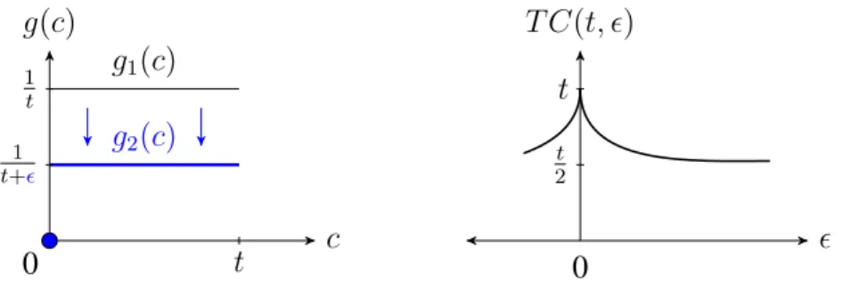
If the players have the same valuationv, then Hillman and Riley (1989) show that in equilibrium each player mixes uniformly with densityg(x) = 1v over the interval[0, v]. The auctioneer expects to collect´0v 1vxdx = v2 from each player, and hencevoverall. There will be full surplus extraction by running an APA when there are symmetric players and complete information. Relaxing either symmetry between players or complete information5will cause this result not to hold. Additionally the APA is triviallyex-postefficient since both players are identical and one of them receives the prize with certainty.
3.2.2 The Assimilation Effect: A First Look
Now I introduce asymmetry into the complete information environment. Now the valuation of playeri isvi (i = 1,2), where without loss of generality letv1 < v2. Hillman and Riley (1989)
were the first to show that in equilibrium players 1 and 2 will both mix uniformly over[0, v1]with
densities g1(x) = v1
2 and g2(x) = 1
v1 respectively. Exactly like the all-pay auction where types
are drawn from some absolutely continuous distribution, in the all-pay auction with finite types asymmetry between the players causes inefficiencies. With positive probability the player with the lower valuation wins, though the probability of this happening converges to 0 as asymmetry is increased.
In equilibrium, each playeri’s mixing density is set equal to the reciprocal of the opponent’s valuationvj:gi(x) = v1
j. This ensures that playeriis indifferent between increasing or decreasing
his bid over the equilibrium support[0,min{v1, v2}]. The marginal benefit of bidding more is equal
5With private information, the auctioneer will collect anex-antefull surplus, i.e. the total expected revenues will
to the marginal cost for bids over this region. When a player becomes stronger,hewill not change his behavior but his opponent will change her behavior. I will later show that with incomplete information asymmetry will cause both player’slowertypes to face different competition. So with incomplete information, there also exist feedback effects that change behavior for both players.
Note that the total weight expended by the weaker player (i.e. player 1) is strictly less than 1. Hence player 1 has “leftover” weight of(1−v1)×v12 = v2v−2v1. This residual weight must be placed
as an atom at 0 in equilibrium. Increasing the degree of asymmetry between the players causes the weaker player to shift more weight from an interval over positive bids to an atom at 0. I say that in this case, due to the presence of increased competition one of the players is discouraged from bidding as much as before. This will be precisely the opposite intuition as the incomplete information case, where stronger competition induces players to bid more. The reason is that with only one type a piece, equilibrium matchups (there is only one) are fixed. The stronger player realizes that the weaker player is not willing to bid more and hence leaves his behavior unchanged. The weaker player therefore cannot bid more and is thus forced to not bid at all with positive probability.
There are slightly different comparative statics if one of the players is made weaker ceteris paribus. The equilibrium support decreases. Not only will the weaker player increase the size of her atom at 0 (thus decreasing revenues), but the stronger player will also on average bid less since he is mixing uniformly over a smaller interval. In this paper I focus on the less intuitive comparative static of making one player stronger, though the case of making a player weaker follows easily from my results.
It follows from the above that asymmetry of any form, meaning an increase inv2 −v1 keeping
one of the valuations fixed, will decrease expected revenues. The weaker player (with valuation v1) will generate revenues ofRev2C ≡ v2
−v1
v2 ×0 +
´v1 0
1
v2xdx = v21 2v2 <
v1
2. The stronger player
(with valuationv2 > v1 ) will generate revenues ofRevC1 ≡
´v1 0
1
v1xdx= v1
2 < v2
2 . Hence for any
valuations v1 andv2, with 0 < v1 < v2, the total expected revenues collected from both players
under a complete information all-pay auction isRevC(v
v2 1 2v2 +
v1 2 =
v1(v1+v2) 2v2 .
Note thatRevC(v1, v2)< v1+v2 2, meaning that the auctioneer will not be able to extract full
sur-plus out of the APA when there is asymmetry between the players. Also note thatRevC(v1, v2)<
v2, wherev2 would be the expected revenues collectedif both players have identical valuations of
v2. Hence if one of two identical players with valuationv2 is made weaker (i.e. now has valuation
v1 < v2), thenceteris paribustotal expected revenues must decrease. This is not a surprising result
as lower valuations would suggest the player is not willing to exert as much costly effort and so will bid less on average. The surprising result is that RevC(v1, v2) < v1 as well, meaning if one
of two identical players with valuationv1 is made stronger (i.e. one now has valuationv2 > v1),
revenues will actually decrease. I collect these results in the following proposition.
Proposition 3 Let players have valuations v1 = v and v2 = v +a, where a ∈ R. Then as a
function ofa, total expected revenuesRevC(v, v +a)have a global maximum ata = 0. Further RevC(v, v+a)is increasing inv for a fixeda.
Proof 5 Suppose first that initially that both players have valuationv, and then player 2’s valua-tion increases fromv → v+afor some a > 0, holdingv1 constant at v1 = v. The equilibrium
support will not change for both players. Only the density for the weaker player will change, namely it will decrease. The residual weight will of course be placed as an atom at 0. Total rev-enues in this case can be computed from to beRevC(v, v +a) = v
2
2(v+a) + v
2, which are strictly
decreasing and convex in a when a ∈ [0,∞]. If on the other hand player 2 is made weaker by a >0, i.e.v1 =vbutv2 =v−a, revenues will beRevC(v, v−a) = v−2a+(v
−a)2
2v , which are also
in strictly decreasing and convex whena >0. Hence revenues decrease at an increasing rate ina.
x g(x)
1 v+
g1(x)
g2(x)
v 0
1 v
v
v 2
Revc(v, v+)
0
Figure 3.1: Complete Information Equilibrium and Revenues
see that asymmetry in the value ofacauses a sharp change in revenues. Adding incomplete infor-mation may also sharply change expected revenues, but in a different way. There exist families of type space distributions , arbitrarily close to the (degenerate) complete information distributions, such that the change in revenues in the family of these distributions is uniformly bounded above some positive constant. Yet with complete information distributions, asymmetry must mean that the change in revenues is negative. Hence it is possible to construct a sequence of type space dis-tributions that converge to the complete information distribution, yet the effects of asymmetry on revenues do not converge. It is in this sense that I mean the comparative statics are not continuous with respect to information. Small amounts of incomplete information may completely change how the auctioneer feels about asymmetry.
In summary, asymmetry is unambiguously bad for revenues in the complete information APA. Making the weaker player even weaker discourages the player from placing weight on positive bids. With positive probability asymmetry causes the weaker player to “give up”, i.e. bid nothing. The stronger player never increases his bid because he will only bid up to what his opponent is willing to bid. Asymmetry may actually reduce the expected bid of the stronger player.
3.3 Private Information Comparative Statics (Valuations)
mix over higher disjoint intervals. This implies that if a lower type’s interval is shifted up, and hence bids more on average, then a higher type’s interval is also shifted up and hence bids higher, ceteris paribus.
Without loss of generality order the types of playerifrom smallest to largest:Ti ≡ {ti,1, ti,2, . . . , ti,n}
with corresponding probabilities{pi,1, pi,2, . . . , pi,n}. In other words,ti,1 ≤ti,2 ≤. . .≤ti,n. Note
that I assume players that can have an equal number of types, but this has no bearing on the results. As long as each player has afinitenumber of types, which includes the complete information case, all of the qualitative results will go through. I can also assume that each player can have only strictly positive valuation (i.e. ti,1 > 0) because any type with a valuation of zero has a strictly
dominant strategy to bid 0 with probability 1. These types will have no bearing on the behavior of the other types nor the comparative statics which we develop later.
3.3.1 Review of Equilibrium Structure
Recall from chapter 1 that in equilibrium each type of each player will mix (piecewise) uniformly over an interval. Each change in uniform density corresponds to a new matchup, i.e. a new type of the other player that is mixing over the type’s interval. If typev1,k is matched up with typev2,m,
the equilibrium densities are pinned down so that each type is indifferent over their interval of bids. The density of player 1 is chosen so that player 2 is indifferent and vice-versa. In equilibrium these densities are
g1,k(x) =
1 p1,kv2,m
g2,m(x) =
1 p2,mv1,k
. (3.1)
is not always the stronger player’s density. The other density must decrease. If a density increases, the length of the interval over which the player is mixing must compensate and decrease in order that probability is well defined. This is ultimately the cause of the assimilation effect, whereby a player responds to asymmetry by increasing his density and ultimately “compressing” his equi-librium interval of bids. Since the lower bound of bids is fixed at 0, this effect tends to decrease revenues. If a density decrease, the player must “stretch” his interval of equilibrium bids, thus increasing expected bids.
3.3.2 Symmetric Equilibrium Benchmark
Suppose that players are symmetric, i.e. that v1,k = v2,k = vk and p1,k = p2,k = pk for all
k = 1, . . . , n. If player i’s realized type is vk, then he will mix uniformly over [bk−1, bk] with
densitygk(x) = p1
kvk, whereb0 = 0andbk = Pk
r=1prvr. Expected revenues from each player are
thenPnk=1pk
´b k
bk−1gk(x)xdx
=Pn k=1pk
b k+bk−1
2
=Pn k=1pk
pkvk
2 +
Pk−1 r=1prvr
. 3.3.3 Asymmetric Equilibrium: The Assimilation and Stacking Effects
With asymmetric players the (unique) equilibrium in an incomplete information APA will not have a neatly written closed form in general. Fortunately the equilibrium construction is easy to describe. Szech (2012) was among the first to extend Hillman and Riley (1989) to private information games, though only with two types. Later Siegel (2013) extended the results for an arbitrary number of finite types (and also inter-dependent valuations, which are not considered here). I use the equilibrium construction of Siegel (2013) to study the comparative statics of the underlying type spaces.
As in chapter 2, we say that typev1,k of player 1 and type v2,m of player 2are matched up if
the intersection of their equilibrium supports is non-empty. More easily stated, each type mixes over an interval in equilibrium. If the intervals of v1,k andv2,m overlap we say they are matched
in general one type fills up before another (with probability 1). Since each type cannot expend more than 1 in weight/probability, there is nothing more this type can do. Thus one highest type will typically have residual weight that is used against the second highest type of the other player. When a matchup is formed one type has exactly a weight of 1 to fill and the other has a weight less than or equal to 1. The distribution of the type space pins down the densities for the matched up types, where in general types will have different densities and hence “fill” at different rates. One type (sayti,k) fills up its weight first6, then a new matchup is formed with the filling player’s next
highest type (ti,k−1 andtj,m) , nowti,k−1has a weight of 1 to fill andtj,mhas some weight strictly
less than one to fill, etc. Monotonicity is crucial to the construction, and as I show later, to the comparative statics of the equilibrium.
A comparative static in this chapter means a change in a type space distribution, specifically a shift in the c.d.f. Fi of a player’s type space. In this dissertation I restrict attention to changes in
Fi where one player is made unambiguously stronger in a first-order stochastic dominance7sense.
Thus I rule out situations where a player’s minimum valuation is increased ( and hence made stronger) but also the same player’s maximum valuation is decreased ( and hence made weaker).
With finite types, there are only three ways that a player can experience a first order stochastic shift in his type space (and hence be made stronger) ceteris paribus : (1) a player’s valuation may increase, (2) the probability of the player having high valuations may increase(and thus the probability of having a low valuation decreases), or (3) some combination or compounding of the first two effects. In the upcoming sections, I consider each of these comparative statics on type space distributions that are initially identical. I show that even the simplest of asymmetries between players can have complex effects on behavior. In a later section I will discuss the qualitative changes that will take place when more than one parameter in the type space has changed.
6It could be that the types fill up exactly together, though this happens with probability 0. Even if this were to
happen the construction can still be applied though.
First I consider changes in equilibrium behavior when one of a player’s valuations is increased, ceteris paribus. It is useful to separate the cases into increasing the lowest valuation and increasing any other valuation. Increasing a player’s lowest valuation in the private information environment, ceteris paribus, will have qualitatively the same features as the complete information environment. Increasing other (higher) valuations, however, will introduce new features that are not seen in the complete information environment.
Increased Lowest Valuation≈Complete Information Comparative Statics
Suppose that the players are initially symmetric but thenv1,1 is increased by some small >0
ceteris paribus, so thatv1,1 =v1+whilev2,1 =v1. Following the equilibrium construction, the
matchups and densities (and hence interval lengths) will remain unchanged for all but the lowest types of both players. The densities for the lowest types will beg1,1(x) = p1
lvl andg2,1(x) =
1 pl(vl+)
for players 1 and 2 respectively. The length of the interval corresponding to this matchup does not change (since v1,1 can still fill up his weight first with the same length of p1v1), and hence the
bidding intervals for all types do not change. Since no more (lower) types of player 1 remain with whichv2,1can be matched,v2,1’s extra weight must be placed as an atom at 0.
Hence all types of both players behave exactly the same after the asymmetry is introduced with the exception of the lowest type of the weaker player (v2,1), who bids strictly less. Overall total
expected revenues decrease, as in the complete information case. The stronger player does not increase his bidding even though he desires the object more because he doesn’t have to. The weaker player is unwilling to bid more as well and so in equilibrium the stronger player will not bid more. Revenues also decrease when one of the players is made weaker. I summarize these results in the following proposition.
Proposition 4 Let bidders be symmetric except that v1,1 = v1 +a and v2,1 = v1, where a ∈
[−v1, v1]. Then as a function ofa, total expected revenues are strictly increasing inawhena < 0
and strictly decreasing whena > 0. Hence as a function ofa, wherea ∈[−v1, v1], total expected
Increased Non-Lowest Valuation6≈Complete Information Comparative Statics
Now consider the more general case of increasing a valuation for a type that is not the lowest for a player. Suppose that players are symmetric except thatv1,kis increased by >0for player 1ceteris
paribus, where k > 1. Using the equilibrium construction, none of the matchups and interval lengths for the types greater thanv1,kwill be changed. However, it will be the case that even though
the lengths of the intervals for these larger types is unchanged, their absolute position will be changed8. Now consider the matchup ofv1,k againstv2,k. The densities for this matchup are again
pinned down to beg1,k(x) = p1
kvk andg2,k(x) =
1
pk(vk+). Typev1,k will be able to fill his weight in
an interval of lengthpkvk. Nowv2,k will have some leftover weight of1−(pkvk)p 1
k(vk+) =
vk+.
Unlike the previous case however, there isa type of player 1, namelyv1,k−1, towards whichv2,k
can apply her remaining weight in a new matchup.
Before proceeding further in the equilibrium construction, some notation is needed. If typekof player 1 and typemof player 2 are matched up, the length of the interval where they are matched up will be denoted asLk,m. Hence so far in the equilibrium construction we know thatLr,r=prvr
for allr≥k.
A new matchup is now formed between v1,k−1 and v2,k. Previously only each type’s mirrored
image was his matchup. As we will shortly see, the pattern now will be that all of player 1’s remaining types face the mirrored type and also the next largest type. In other words, type v1,r
will facev2,r andv2,r+1 whenr < k. Hence all of player 1’s remaining types are matched up with
stronger competition. Similarly each type of player 2 now faces the same mirror type, and also weaker competition.
I consider a few iterations of the equilibrium construction to emphasize the changing matchups. This is crucial to understanding the encouragement and discouragement effects. The densities for this new matchup are g1,k−1(x) = p 1
k−1vk and g2,k(x) =
1
pkvk−1. As before, the length of
the interval corresponding to this matchup will depend upon how long of an interval v2,k needs
8This is analogous to the two intervals[1,2]and[5,6]. But have length 1, but the lower and upper bounds have
to fill the remaining weight from the v1,k matchup 9. To fill a weight of vk+ with a density of
g2,k(x) = p 1
kvk−1, a length of
pkvk−1
vk+ is needed. Hence the length of the new interval from the
matchup ofv1,k−1andv2,kisLk−1,k = pvkvk−1
k+ .
In the next matchup ofv1,k−1andv2,k−1, it will be the case thatv1,k−1 has expended some of his
weight. He has weight of1−pkvk−1 vk+
1
pk−1vk when he facesv2,k−1. Since these types have the same
densitiesg1,k−1(x) =g2,k−1(x) = pk−11vk−1, butv1,k−1 has less weight to fill,v1,k−1 will be able to
fill first. The length of the interval required for this matchup isLk−1,k−1 =pk−1vk−1 −pk(vk−1) 2
(vk+)vk .
The first term represents the length of the interval in the symmetric case. Hence the length of this interval for the matchup ofv1,k−1 andv2,k−1 has been decreased (sincev1,k−1 has already used up
some of his weight).
We consider one more iteration of this process before generalizing the results. Now thatv1,k−1
has filled up his weight againstv2,k−1, a new matchup ofv1,k−2 andv2,k−1 is formed. Nowv2,k−1
has remaining weight of1−Lk−1,k−1 × p 1
k−1vk−1 =
pkvk−1
(vk+)pk−1vk. Densities for this new matchup
are pinned down to be g1,k−2 = p 1
k−2vk−1 and g2,k−1 = 1
pk−1vk−2, where we have suppressed the
argument (x) of the density because the density is constant. If is small enough, then v2,k−1 will
indeed be able to fill up her weight before v1,k−2 does. This will require a length of Lk−2,k−1 = pkvk−1vk−2
(vk+)vk .
Now v1,k−2 will be matched up with v2,k−2, where v1,k−2 has a weight of 1 − Lk−2,k−1 × 1
pk−2vk−1 = 1−
pkvk−2
(vk+)vkpk−2. Both densities are the same at g1,k−2 = g2,k−2 = 1
pk−2vk−2. Of
course v1,k−2 will be able to fill up his weight first since they have the same density but v1,k−2
has weight strictly less than 1 to fill. The length required to fill up his weight against v2,k−2 is
Lk−2,k−2 =pk−2vk−2−
pk(vk−2)2 (vk+)vk .
Continuing in this manner for all the rest of the types we see that the asymmetry will have an effect that ripples through all of the remaining (i.e. lower) types matchups and densities. The equilibrium construction will continue untilv1,1 fills up his weight against v2,1, leavingv2,1 with
9For very small values in,v
leftover weight to be placed as an atom at zero. In general, ifr < kthen typev1,rwill be matched
up with typesv2,r+1 andv2,r. The lengths of these intervals will beLr,r+1 = p(vkvrvr+1
k+)vk andLr,r =
prvr− pk(vr) 2
(vk+)vk . Intuitively a small asymmetry changes the equilibrium in a small manner in that
the size of the interval of the new matchups areLr,r+1 < . Since there are a finite number of types,
this implies that for small enough >0the change in revenues can be made arbitrarily small. One final piece of notation is required before generalizing the change in the stronger player’s behavior. For types r < k, define br =
Pr
t=1Lt,t +Lt,t+1 as the upper bound of type v1,r’s equilibrium
support.
Corollary 1 Forr < k,
d
dLr,r() =−
pk(vr)2
(vk+)2
<0 (3.2)
d
dLr,r+1() =
vrvr+1pk
(vk+)2
>0 (3.3)
d
dbr() = pk
(vk+)2 r
X
t=1
vt(vt+1−vt)>0. (3.4)
The above corollary shows that the interval over which all of player 1’s types mix is shifted upwards while only the intervals of player 2’s highest types are shifted upwards. The lowest types of player 2 compress their equilibrium intervals. I now summarize the behavior of the stronger player after the asymmetry is introduced.
Proposition 5 Let players be symmetric exceptv1,k = vk+andv2,k = v)k, where k > 1and
>0. Equilibrium behavior of player 1 (the stronger player) is characterized by:
Typesr < k Typev1,r will mix over[br−1, br−1 +Lr,r]with densityg1,r = pr1vr and over[br−1+
Lr,r, br]with densityg1,r = prv1r+1.
Typek The perturbed type,v1,k, will mix over[bk−1, bk−1+pkvk]with densityg1,k = pk1vk.
Typesr > k Typev1,r will mix over[bk−1+Pr −1
t=kptvt, bk−1+
Pr
Calculation of expected revenues for each type of player 1 is tedious but straightforward. Sim-ilar to the complete information environment, revenues are not differentiable at = 0, so we focus instead on the right hand side derivative, which does exist. Since > 0, by construc-tion we are implicitly considering comparative statics when players become stronger. If < 0 the equilibrium would be qualitatively different in that there would be different matchups, inter-val lengths (Lk,m’s), and densities. When I write the derivative of revenues,
dRevi,r(0)
d , I mean dRevi,r(0)
d ≡lim&0
Revi,r()−Revi,r(0)
. In this context, it is equivalent to differentiating the revenues
with respect toand then take the limit as→0.
LetRevi,r()be the product of the conditional expected revenue collected (conditional on type
r realized for player 1) and the probability of the type. In other words, Revi,r() is type vi,r’s
contribution to expected revenues. The sum Pn
t=1Rev1,t() then represents the total expected
revenues collected from player 1. All of the comparative statics for the strong player are collected in the following proposition.
Proposition 6 Let players be symmetric except thatv1,k =vk+andv2,k = vk for some > 0.
The rate of changes in revenues for player 1 are
dRev1,t()
d =
pkpt
v2 k
t−1
X
r=1
vr(vr+1−vr)>0 if t≤k (3.5)
dRev1,t(0)
d =
ptpk
v2 k
k−1
X
r=1
Proof 6
Rev1,r() =pr
ˆ b1,r−1+Lr,r
b1,r−1
1 prvr
xdx+
ˆ b1,r
b1,r−1+Lr,r
1 prvr+1
xdx
!
(3.7)
=Lr,r(2b1,r−1 +Lr,r) 2vr
+Lr,r+1(2b1,r −Lr,r+1) 2vr+1
(3.8) dRev1,r()
d =
1 vr
Lr,r
dbr−1
d +br−1 dLr,r
d +Lr,r dLr,r d (3.9) + 1 vr+1 Lr,r+1 dbr
d +br
dLr,r+1
d −Lr,r+1
dLr,r+1
d
(3.10) dRev1,r(0)
d =
1 vr
"
prvr(
pk
v2 k
)
r−1
X
t=1
vt(vt+1−vt) + ( r−1
X
t=1
ptvt)(−
pkvr2
v2 k
) +prvr(−
pkv2r
v2 k ) # (3.11) + 1 vr+1 "
0 + (
r
X
t=1
ptvt)
vrvr+1pk
v2 k
−0
#
(3.12)
=prpk v2
k r−1
X
t=1
vt(vt+1−vt)−
pkvr
v2 k
r
X
t=1
ptvt−prvr
!
− prpkv
2 r
v2 k
+ vrpk v2
k r
X
t=1
ptvt
!
(3.13)
=pkpr v2
k r−1
X
t=1
vt(vt+1−vt)>0 (3.14)
Now consider the revenues of the perturbed typev1,k, who mixes over[bk−1, bk−1 +pkvk]with
densityg1,k = p1
kvk. Revenues (again premultiplied by the probability) for this type are
Rev1,k() = pk
ˆ bk−1+pkvk
bk−1
1 pkvk
xdx= p
2 kvk
2 +pkbk−1 (3.15)
Directly differentiating we get
dRev1,k()
d =pk dbk−1
d =pk
pk
(vk+)2 k−1
X
t=1
vt(vt+1−vt)
!
>0. (3.16)
lower and upper bounds of the intervals are both increased:
Rev1,r() =pr
ˆ bk−1+Prt=kptvt
bk−1+ Pr−1
t=kptvt
1 prvr
xdx= 1 2vr
prvr(2bk−1+ 2 r−1
X
t=k
ptvt+prvr) (3.17)
dRev1,r(0)
d =pr
dbk−1
d =
prpk
v2 k
k−1
X
t=1
vr(vr+1−vr)>0. (3.18)
Hence the lower types of the player that is made stronger all bidmoreon average. This is the assimilation effect. Player 1’s lower types see tougher competition and respond by stretching their equilibrium intervals and ultimate bidding more. In contrast player 1’s higher types see the same competition but bid more because of thestacking effect. Since the lower types are bidding more, the higher types must bid more as well. Hence we can say that expected revenues collected from every type of the stronger player (i.e. player 1) will increase, but for different reasons.
Now consider the weaker player, i.e. player 2. Following a similar approach we partition the types of player 2 into thekth type, types belowk, and types abovek. The matchups and densities for types abovek will not change for bidder 2. Hence all of the results that are true for bidder 1’s types abovek are also true for bidder 2’s types abovek. The largest types of the weaker player will bid more also because of thestacking effect. The first matchup to change will be typev2,k.
In response tov1,k becoming stronger, v2,k responds by decreasing her density tog2,k = p 1
k(vk+).
In equilibrium, type v2,k will mix over [bk−1 −Lk−1,k, bk−1] with densityg2,k = p 1
kvk−1 and over
[bk−1, bk−1+Lk,k]with densityg2,k = p 1
k(vk+).
Proposition 7 Suppose initially that bidders are symmetric, i.e. v1,t =v2,t =vtandp1,t =p2,t =
pt for allt = 1, . . . , n. If for somek, v1,k is increased by > 0tov1,k = vk+, then the lowest
dRev2,t(0)
d =
ptpk
v2 k
t−1
X
r=1
vr(vr+1−vr)−vt2
!
<0 if t < k (3.19)
dRev2,t(0)
d =
p2 k
v2 k
k−1
X
r=1
vr(vr+1−vr)−
v2 k
2
!
<0 if t =k (3.20)
dRev2,t(0)
d =
ptpk
v2 k
k−1
X
r=1
vr(vr+1−vr)
!
>0 if t > k (3.21)
We present a useful Lemma before characterizing revenues for player 2.
Lemma 4 Let0≤v1 < v2 <· · ·< vm, wherem ≥2. For a fixedvm, the sumPm −1
r=1 vr(vr+1−vr)
is maximized whenvr = mrvm forr = 1, . . . , m−1. Further, at the maximumPm −1
r=1 vr(vr+1 −
vr)≤ v 2
m
2 .
Proof 7 To show thatPm−1
r=1 vr(vr+1−vr)is maximized whenvr = r
mvm forr= 1, . . . , m−1, I
show that the sum has a strict local maximum by taking first and second order conditions, showing that all of the leading principal minors of the Hessian matrix alternate in sign, with the first being negative. The first order conditions of the sum are
v1 : v2 −2v1 = 0 (3.22)
v2 : v1 +v3−2v2 = 0 (3.23)
v3 : v2 +v4−2v3 = 0 (3.24)
..
. (3.25)
vr : vr−1+vr+1−2vr = 0 (3.26)
..
. (3.27)
vm−1 : vm−1+vm+1−2vm = 0 (3.28)
Solving this system of equations yields solutions of the formvr = mrvk. The Hessian matrix is