Mining sensor data from complex systems

(1)

Cover Page

The handle http://hdl.handle.net/1887/37027 holds various files of this Leiden University dissertation.

Author: Vespier, Ugo

(2)

Mining Sensor Data from

Complex Systems

Proefschrift

ter verkrijging van

de graad van Doctor aan de Universiteit Leiden, op gezag van Rector Magnificus prof.mr. C.J.J.M. Stolker,

volgens besluit van het College voor Promoties te verdedigen op dinsdag 15 December 2015

klokke 12.30 uur

door

Ugo Vespier

(3)

Promotor: prof. dr. J. N. Kok Co-promotor: dr. A. J. Knobbe

Overige leden: prof. dr. E. Keogh (University of California, Riverside) dr. J. Gama (University of Porto)

(4)

iii

(5)

(6)

Chapter 1 Introduction

Over the last decades, the advances in computational power, storage technol-ogy and sensor networks have made data an abundant resource [79]. Today, virtually everything, from natural phenomena to complex artificial and physi-cal systems, can be measured and the resulting information collected, stored and analyzed in order to gain new insight, optimize existing processes or both.

The term Big Data has gained popularity, in academia, industry and the public opinion, to describe the opportunities and the challenges connected to this huge explosion in data availability [64]. In a report by IDC [33], the au-thors estimate that the total amount of data in the digital world will amount to 40.000 exabytes1 _{by the end of 2020, almost doubling its size every year.}

The data sources are diverse, ranging from user-contributed material on so-cial networks (i.e. posts, tweets and status updates) to consumer behavioral data collected by online retailers such as product views and purchases. In particular, advances in measuring technology and sensors networks [3, 16] greatly contributed to the explosion of data. The adoption and deployment of measurement systems for all sorts of industrial, commercial and consumer applications, is paving the way to important opportunities for monitoring and analyzing all kinds of systems over time at a level of detail never experienced

1_{This equates to 4}

·1022 _bytes.

(11)

before.

In fact, sensing technology and the ability to manage big data represent a fundamental improvement in our ability to measure complex systems. Mul-tiple types of sensors, high sampling rates, advances in noise reduction tech-niques, to cite a few, are all improvements that are contributing to making progressively better representations of systems in data.

As a result, new challenges in the analysis and visualization of this large amount of sensor data have emerged and, over the last decade, the ef-forts of the research community to provide solutions to these problems have soared [1]. Methods and algorithms, in fact, will have to advance in order to cope with the increased complexity of the time series datasets available and to improve the ability to learn from the greater level of detail present in them.

A side effect of the exponential explosion of data collection is that labeled

information will be an increasingly scarce resource in the future, as it is ex-tremely costly to produce labeled datasets in relation to the current rate of data growth. Because of this, the task of extracting structured information from unlabeled data is of paramount importance when dealing with the chal-lenges posed by big data. The algorithms and methods presented in this thesis are designed to work in this scenario where novel insights have to be extracted in an unsupervised way.

In particular, the focus of this thesis is the analysis of complex sensor data in the form of time series. Time series are sequences of observations sam-pled periodically over time. We approach the analysis of such data from

a data mining perspective, with the end goal of extracting previously

(12)

3

In this thesis, we introduce data mining and visualization methods for large time series data collected from complex physical systems by means of sen-sors.

Our work is motivated by InfraWatch [55], a Structural Health Monitoring project centered around the management and analysis of data collected by a large sensor network deployed on a highway bridge. The sensor network comprises strain, temperature and vibration sensors, sampling continuously at 100 Hz. A highway bridge is a complex system and so is the data collected. The behaviour of the bridge, and consequently the properties of the data, is affected by external factors such as the temperature, weather conditions, traffic activity and deterioration of the concrete. Moreover, InfraWatch data contains repeated patterns at different resolutions due to the bridge’s re-sponse to recurring events such as passing vehicles or traffic jams. Because of these characteristics, InfraWatch is an ideal testbed for evaluating the methods we introduce.

In this thesis, we will develop and discuss solutions to the following fun-damental questions when dealing with large and complex time-series data collected from sensors like the one provided by InfraWatch:

• What are the relevant temporal scales of analysis for a given time series?

• Which are the recurring multi-scale patterns present in a given time series?

• How can we effectively model and recognize events in time series data?

• How can we support efficient and interactive visualization of massive time series data?

(13)

temporal scales of analysis and introduce a decomposition of the original time series such that every component represents a single phenomenon at its characteristic scale. The goal of the method is to find the underlying factors that explain the input data.

These multiple phenomena, moreover, are often characterized by the presence of patterns that repeat over time and reflect their effect in the data. Consider again the strain sensor example. The effect of traffic jams will produce similar recurring patterns in the data, for example every morning during rush hour. The same would happen with the effect of passing vehicles, although they will appear at a shorter time scale (in the order of seconds) and potentially superimposed on the traffic jam patterns. We will introduce a method to mine recurring patterns, so-called motifs in the literature, from time series data at multiple temporal scales.

The third research question addresses the problem of clustering time series subsequences in order to model and recognize fixed-length events in the data. Time series clustering has proven to be a difficult task, as it is hard to model the subsequence space properly without introducing artifacts in the results [49]. We will introduce a novel distance measure to cope with this problem.

Finally, we will address the problem of massive time series visualization. Al-though visualization is not directly related to data mining, it is a fundamen-tal task in every data science project, especially to support the exploratory phases and build an idea of the data at hand. When exploring and visu-alizing a dataset, interactivity is important as it permits testing ideas and assumptions quickly without having to wait excessive periods. We will see how we made the interactive visualization of terabyte-sized datasets possible by introducing an ad-hoc storage scheme for time series, which effectiveness has been proven by a real world software package called VizTool.

(14)

5

the need for effective visualization, are general challenges shared among all complex physical and artificial systems measured by sensor networks.

The methods and algorithms introduced in this thesis combine concepts from data mining, signal processing, and information theory. In particular, in order to formally characterize the concept of temporal scales, we will make use of concepts from the field of signal processing, such as the theory of scale-space [103, 62].

As we are interested in extracting new insights from the data, such as the relevant temporal scales and the recurring events, we approach the problem from a compression standpoint. The idea of using concepts from the theory of compression in order to learn new facts about the structure of a dataset has been widely considered and explored in the literature [82, 105]. Data compression techniques geared towards learning have been employed for cat-egorizing text [29], clustering data [17], devising similarity measures [99, 52], in genomic analysis [36], data discretization [57], pattern mining [100, 68, 84], stream mining [89], and as the base of parameter-free data mining meth-ods [51].

(15)

1.1 Thesis Outline

Below, we give a brief outline of the dissertation, summarizing the contents of the following chapters. As most chapters are based on previous publications by the author, we also give the appropriate references to them when this is the case.

In Chapter 2: Sensor Data and Applications, we give the main moti-vations behind this work and introduce the InfraWatch project.

InChapter 3: Preliminaries and Background, we introduce fundamen-tal material and concepts that will be used throughout the rest of the thesis, especially in Chapter 4 and Chapter 5.

In Chapter 4: Identifying the Relevant Temporal Scales, we discuss a method for discovering the most relevant scales of analysis, and their cor-responding scale components, in time series data. This work was published in the following paper [96]:

Vespier U., Knobbe A., Nijssen S., and Vanschoren J.,MDL-based

Analysis of Time Series at Multiple Time-Scales, in Proceedings

ECML-PKDD 2012, Bristol, UK.

This work is also part of the following book chapter [95]:

Vanschoren, J., Vespier, U., Miao, S., Meeng, M., Cachucho, R., Knobbe, A.,Large-scale sensor network analysis — Applications

in structural health monitoring, in Big Data Management,

Tech-nologies, and Applications, IGI Global, 2013

InChapter 5: Mining Variable-Length Motifs at Multiple Scales, we introduce a method for mining variable-length, and potentially overlapping, motifs at multiple temporal scales in sensor-based time series data. This work was published in the following paper [98]:

Vespier, U., Knobbe, A., Nijssen, S.,Mining Characteristic

Multi-Scale Motifs in Sensor-Based Time Series, in Proceedings CIKM

(16)

1.1. THESIS OUTLINE 7

InChapter 6: Subsequences Clustering for Events Modeling, we dis-cuss a distance measure and an associated method for the effective clustering time-series subsequences for events modeling. This work was published in the following paper [97]:

Vespier, U., Knobbe, A., Vanschoren, J., Miao, S., Koopman, A., Obladen, B., Bosma, C., Traffic Events Modeling for Structural

Health Monitoring, in Proceedings IDA 2011, Porto, Portugal.

This work is also part of a book chapter [95]:

Vanschoren, J., Vespier, U., Miao, S., Meeng, M., Cachucho, R., Knobbe, A.,Large-scale sensor network analysis — Applications

in structural health monitoring, in Big Data Management,

Tech-nologies, and Applications, IGI Global, 2013

In Chapter 7: Interactive Time-Series Visualization, we introduce a method and a software platform for visualizing terabyte sized time-series dataset. This work was published in the following paper [6]:

(17)

(18)

Chapter 2 Sensor Data and Complex

Systems

In this chapter, we discuss the context of this dissertation and the motivation behind the presented work. We also present the InfraWatch project, the main application and testbed for the methods discussed in the next chapters.

2.1 Big Data

As mentioned, the term Big Data has received a lot of attention over the last years [64], although it is often cause of confusion as its meaning is not always well-defined in all contexts. Big data is a broad term that refers to the challenges in managing and analyzing large quantities of data.

A widely accepted definition of Big Data has been given by Gartner’s analysts Beyer and Laney in a 2012 industry report [11] where the authors define the term in relation to three main challenges:

Volume The ever-growing amount of data that institutions and companies have to deal with offers serious challenges in terms of data management and storage. Real-world examples range from the data collected by astronomers with radio telescopes, to the massive amount of messages

(19)

exchanged nowadays on social networking platforms such as Facebook and Twitter. Novel storage and indexing methods, able to cope with this huge amount of collected information, need to be employed.

Velocity A second important challenge is related to how long it takes to process incoming data. For example, a credit card institution analyzing massive streams of incoming transactions would like to detect potential fraud without delay. Real-time processing methods are needed in order to cope with the velocity challenge.

Variety Last but not least, Big Data comes in any type, both in structured and unstructured form. Text, audio, video, sensor data, log files, and combinations of these, are examples of data types found in Big Data applications [15]. The development of methods able to cope with this broad variety of data is another challenge posed by Big Data applica-tions.

A great extent of the efforts aimed at solving big data problems revolve around these three challenges, as well as a broad range of applications across several science fields and industries. Sensor networks and monitoring is an important one and represents the main focus of this thesis. In particular, the rise of the Internet of Things [4, 5] is directly connected to the challenges posed by the management and analysis of Big Data.

2.2 Sensor Networks and the Internet of Things

The last two decades have witnessed a tremendous growth in the availability of sensor data collected from a multitude of systems in various application domains [3, 16]. In fact, the wider availability of cheap sensor technology has enabled large sensor networks that continuously monitor and analyze physical systems such as infrastructures, cars [25, 45, 59, 32], airplanes [7, 107, 9, 87] and, last but not least, the human body [14, 83].

(20)

2.2. SENSOR NETWORKS AND THE INTERNET OF THINGS 11

humans and software communicate to achieve common goals by directly in-teracting with the physical world. This paradigm is called Internet of Things (IoT) [35, 5] and several applications of its concepts are already used in production.

In a recent report [72] by McKinsey & Company, the authors categorize IoT applications in three main areas:

• Tracking behavior

• Enhanced situational awareness

• Sensor-driven decision analytics

Companies and institutions are interested, first of all, in tracking and moni-toring products and objects in real-time [54] in order to increase the efficiency of their operations or fine-tune their business or pricing models. Consider, for example, the case of a car insurance company that installs sensors in their cus-tomers’ cars in order to monitor and model the behavior of drivers [90]. Situational awareness [106] is another key application area of the IoT. Large sensors networks, in fact, can be deployed in infrastructures, such as roads, buildings or bridges, or installed in certain areas to report on environmental conditions. Data coming from the sensors can then be used to enhance the awareness of decision makers about the observed events in real-time, especially when data is coupled with tailored visualization technologies. Ultimately, sensor networks can support long-term and complex decision making. In the retail industry, for example, some companies are experi-menting with sensors that continuously monitor shoppers [67, 63] as they move through stores in order to measure how long they stand in front of any given display and correlate it with what they ultimately buy. Data of this kind can help, in the long run, by optimizing store layouts and increase revenues.

(21)

management solutions in order to cope with the large amount of collected data and ensure its effective storage, access and visualization.

Such large amounts of data, on the other hand, represent an opportunity to apply data mining methods to better understand the observed system and get insight into its behavior [1]. Moreover, as these data sources continuously provide data over time, the research community is also focusing on methods and algorithms to analyze information in a streaming fashion in order to provide real-time insights [31].

2.3 Multi-Scale nature of Complex Systems

Sensor networks are often employed to monitor and analyze complex, dy-namic systems, which exhibit non-obvious behavior. An important example are systems affected by several phenomena at different temporal scales. Consider, for example, the electrical system of an apartment whose aggre-gate power consumption is measured by a smart meter [108, 58]. The time series data collected by the smart meter would be affected by all the oper-ational home appliances, heating units and lighting systems in the house. As different home appliances are switched on at different times and have diverse operational durations, their effect on the aggregate consumption can range from short-term spikes, for example in the case of a boiler, to longer, more equally distributed patterns, as for example in the case of a washing machine [73]. For example, the time series in Figure 2.1 shows four days of power usage from an apartment in the Smart* dataset [8]. In the data, there is a clear long-term periodic component due to the cycles of the refrigerator. Shorter-term patterns, however, show up superimposed in the data and cor-respond to activations and deactivations of the various electrical appliances in the house.

(22)

2.4. SHM AND INFRAWATCH 13

00:00:00 12:00:00 00:00:00 12:00:00 00:00:00 12:00:00 00:00:00 12:00:00

1334448000 100

200 300 400 500 600 700 800

Figure 2.1: Four full days of power usage (in watts) from one of the houses in the Smart* dataset [8].

along diverse temporal scales. For example, lunar tides indirectly affects wa-ter pressure following both a half-daily cycle and a longer-wa-term, two-weekly cycle.

Analysing systems such as the ones described above requires methods capable of dealing with the presence of multiple relevant scales of analysis in order to extract insights at all levels and resolutions. This represents one of the main challenges addressed in this thesis.

2.4 SHM and InfraWatch

One relatively recent application of sensor networks and sensor data analy-sis is the monitoring of infrastructural assets such as bridges, tunnels, etc. [21]. In fact, according to a recent survey from the US Federal Highway Commission [28], on average 56% of the assessments to civil infrastructures made by visual inspection are inappropriate, suggesting additional methods of monitoring to guarantee the safety of the assets.

Structural Health Monitoring (SHM) is an interdisciplinary field at the

(23)

fact, the use of advanced sensing and monitoring systems provides the op-portunity to collect real-time information from infrastructures, in order to monitor their performance and to deduce relevant knowledge for decisions on their maintenance demand [26, 86]. Asset owners can use this information to assess the life time perspective of (crucial) infrastructural links and to plan the window within which maintenance can be conducted. When considering the stock of infrastructural assets in view of service-life assessment, monitor-ing and sensmonitor-ing systems are very valuable instruments that can be used to extract actual information about its condition and performance.

In typical SHM scenarios, sensor systems are mounted in or to structures and monitor the environmental as well as the internal condition of the measured system over long periods of time. The collected sensor data is typically continuously analyzed in order to detect inconsistencies or anomalies in how the structure is behaving and notify potential problems in time. Aside from notifying anomalies, SHM systems are also used to monitor and forecast degradation mechanisms in order to plan maintenance in a more informed way.

In the next section, we present a particular SHM project in detail. This project and its data will serve as a testbed for a great extent of the methods and algorithms presented in this thesis.

2.4.1 The InfraWatch project

InfraWatch is a project that is part of a Dutch STW’s funded program called Integral Solutions for Sustainable Construction (IS2C). The program is com-posed of nine research projects with the common goal of setting new stan-dards and advancing the state of the art in the field of sustainable construc-tion and service-life assessment.

As part of the IS2C program, InfraWatch1 _{focuses on sensing, monitoring}

and degradation mechanism from a data analysis perspective. Subject of the project is an important Dutch highway bridge: the Hollandse Brug. The

(24)

Figure 2.2: Picture of the Hollandse Brug, which connects the ‘island’ Flevoland to the province Noord-Holland.

landse Brug is a bridge between the Flevoland and Noord-Holland provinces and is located at the place where the Gooimeer joins the IJmeer (see Figure 2.2). The bridge was opened in June 1969 and National Road A6 uses it. There is also a rail connection parallel to the highway bridge, as well as a lane for cyclists on the west side of the car bridge.

(25)

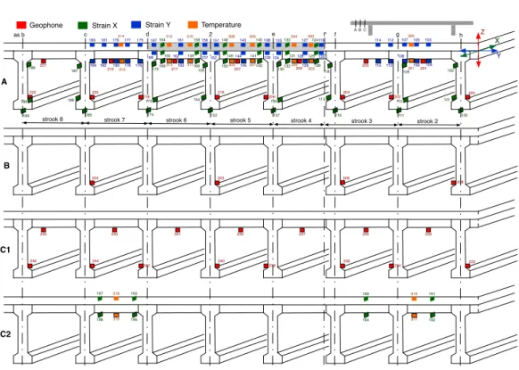
The monitoring system comprises 145 sensors that measure different as-pects of the condition of the bridge, at several locations along the bridge (see Figure 2.3 for an illustration). The following types of sensors are em-ployed [55, 56]:

• 34 ‘geo-phones’ (vibration sensors) that measure the vertical movement of the bottom of the road-deck as well as the supporting columns.

• 16 strain gauges embedded in the concrete, measuring horizontal lon-gitudinal strain, and an additional 34 gauges attached to the outside.

• 28 strain gauges embedded in the concrete, measuring horizontal strain perpendicular to the first 16 strain gauges, and an additional 13 gauges attached to the outside.

• 10 thermometers embedded in the concrete, and 10 attached on the outside.

Furthermore, there is a weather station, and a video-camera provides a con-tinuous video stream of the actual traffic on the bridge. Additionally, there are also plans to monitor the adjacent railway bridge.

The current monitoring set-up is clearly providing many challenges for data management. The 145 sensors are in fact producing data at rates of 100 Hz, which can amount to a gigabyte of data per day. Adding to that is the continuous stream of video.

Project goals and expectations

InfraWatch is, primarily, a Structural Health Monitoring project and its goals are directly related to questions about the observed infrastructure from a civil engineering perspective. The following tasks, in particular, are of importance to the civil engineers involved in the project:

• obtain a summary of the major phenomena affecting the bridge infra-structure over time and their impact.

(26)

A

B

C1

C2

Geophone Strain X Strain Y Temperature

222 221 219 220 217 218 207 216 206 205 203 204 202 201 200 246 245 243 244 241 242 239 240 238 237 235 236 234 233 232

224 223 209

208 188 189 190 187 186 185 172 173 174 155 154 153 135 136 137 118 117 116 109 110 111 102 101 100

183 181 179 177 175 184 182 180178 176

314 164 165 166 158 159 160 167 168 161 163 162 312 313 310 311 156 157 148 149 150 140 141 142 151 152 143 145 144 308 309 306 307 138 139 130 131 132 124 125 126 133 134 127 129 128 304 305 302 303 119 120 114 112 115113

107 105 103 108 106 104 197 198 195 196 318 319 193 194 191 192 316 317 Z X Y

A B C

as b c d 2 e f' f g h

strook 8 strook 7 strook 6 strook 5 strook 4 strook 3 strook 2

300

301 315

Figure 2.3: Diagram explaining the individual sensor placement on the Hol-landse Brug.

quantitative estimate of the structural health of the Hollandse Brug.

• given the current sensor network deployment, obtain a new configura-tion of sensors, possibly employing fewer sensors, that is equivalent or comparable in terms of collected information.

In this thesis, we provide fundamental data mining methods and algorithms that can be employed to design a solution for the tasks above and related tasks involving sensors monitoring and analysis of systems.

Technical challenges

(27)

different temporal scales, the methods and solutions will have to cope with its multi-scale nature. The tasks we are interested in are described below:

• given a sensor-based time series, identify which are the relevant tem-poral scales of analysis.

• given a sensor-based time series, identify which are the recurring pat-terns in the data at multiple temporal scales.

(28)

Chapter 3 Preliminaries and

Background

As discussed in the previous chapters, the primary focus of this thesis is the unsupervised analysis of sensor data collected from complex multi-scale systems. In this chapter, we review the main background concepts and tools that lay the foundations and prepare the discussion for the material in the remaining chapters.

We will start by introducing the concept of convolution and signal filter-ing [85]. As we deal with noisy measurements from real-world sensor net-works, we will show how convolution and filtering can be used to reduce the effect of noise and support several other time series manipulation tasks. Building on the concept of convolution, we will then present a fundamental tool employed in the rest of the thesis that supports the analysis of a time series at multiple temporal scales: the scale-space image [103]. Finally, as our main focus is on the unsupervised modeling of phenomena in time series data, we will introduce the Minimum Description Length principle as our model selection framework of choice [34], motivate its adoption and discuss a simple application of it to noise removal.

(29)

3.1 Preliminaries

We start by giving some fundamental definitions used in this chapter and throughout the thesis. We deal with finite sequences of numerical measure-ments, collected by observing some property of a system with a sensor, and represented in the form of time series as defined below.

Definition (Time Series). A time seriesof length n is a finite sequence of values x=x[1], . . . , x[n] of finite precision1_.

Throughout the thesis, we assume that the measurements are collected at uniformly spaced time points and according to a fixed sampling rate.

In many contexts, it is of particular interest to refer only to certain contiguous portions of a time series or subsequences, as defined below:

Definition (Subsequence). A subsequence x[a : b] of a time series x is defined as follows:

x[a:b] = (x[a],x[a+ 1], . . . ,x[b]), a < b

3.2 Convolution and Filtering

Convolution is arguably one of the most important techniques in signal pro-cessing, for both the one-dimensional (time series) and two-dimensional case (images), and the fundamental operation in linear filtering. From a mathe-matical standpoint, convolution combines two functions to produce a third one, as defined below.

Definition (Convolution). Given two functions f and g, their convolu-tion f_∗gis defined as the integral of their product after one of the functions is reversed and shifted:

(f _∗g)(t) =

Z ∞

−∞

f(τ)g(t₋τ)dτ

(30)

3.2. CONVOLUTION AND FILTERING 21

When referring to the process of filtering, the function f is said to be the signal to be filtered while the function g is called convolution filter kernel. Kernel functions directly define the properties of the filter. Specific kernel functions can be defined for amplification and attenuation, shifting or echoing of a signal. Other classes of kernel functions, as we will see shortly, can be used for low-pass and high-pass frequency filtering.

3.2.1 Convolution and LTI Systems

Although, in the context of this thesis, convolution is mainly used as a fil-tering operation, it is worth mentioning its deep connection with the theory

of linear time-invariant (LTI) systems [85]. A system, defined by an input

signalx(t) and output signaly(t), is said to be linear time-invariant if it sat-isfies the linearity and time-invariance properties. Linearity refers to the fact that a linear mapping exists between the inputs and the output of the sys-tem. More formally, given two inputsx1(t) andx2(t), respectively producing

outputs y1(t) and y2(t), the scaled and summed input a1x1(t) +a2x2(t) will

produce a1y1(t) +a2y2(t), where a1 and a2 are scalars. The property holds

for any arbitrary number of terms.

On the other hand, time-invariance means that the output of the system does not depend on the particular time a given input is applied. In detail, given an inputx(t) and an outputy(t), the delayed inputx(t₋δ) will produce the delayed outputy(t₋δ).

(31)

3.2.2 Discrete Convolution

Although we defined the convolution operation in the continuous domain, in practical cases, however, we deal with finite signals in the discrete domain (time series). The definition of convolution in the discrete case is presented below.

Definition (Discrete Convolution). Given a time series x of length n

and a convolution filter kernel h of length m, the result of the discrete convolution x_∗h is the time series yof length n, defined as:

y[t] =

m/2

X

j=−m/2+1

x[t₋j]h[j]

Note that sincex is finite, x[t₋j] may be undefined. To account for these boundary effects, x is padded with m/2 zeros before and after its defined range.

If not specified otherwise, from now on we will only refer to the discrete case of convolution.

3.2.3 Noise Filtering via Gaussian Smoothing

A common use of the convolution operator is smoothing a signal to remove noise or finer details. Smoothing can be obtained by employing several types of kernels like mean, median and Gaussian. In [12], the authors propose a methodology to mine interesting correlations in multivariate time series data based on generating features obtained by convoluting the input data with different kernels in order to enhance or reduce certain characteristic.

Gaussian smoothing, however, is a common noise filtering technique, as it cuts high frequencies, leaving untouched the low ones. It also has other useful properties as we will see in the next section.

(32)

be-3.2. CONVOLUTION AND FILTERING 23

low:

Gσ =

1

√

2πσ2e

−x2

2σ2

which, in the scope of this thesis, has a mean of 0, standard deviationσ and area under the curve equal to 1.

We can now define Gaussian smoothing as a particular convolution operation employing a Gaussian kernel.

Definition (Gaussian Smoothing). Given a time seriesxof lengthnand a Gaussian kernel Gσ discretized into m values, the result of the Gaussian

smoothing is the time seriesy of length n, defined as:

x[i]_∗Gσ[i]

Note that to capture almost all non-zero values, we definem =_b3σ_c.

The convolution acts as a smoothing filter which smooths each value x[t] based on its surrounding values. The amount of removed detail is directly proportional to the standard deviationσ (and thusm), from now on referred to as the scale parameter. In the limit, when σ _{→ ∞}, the result of the Gaussian convolution converges to the mean of the signal x over the entire period involved.

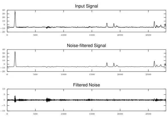
To better picture the effect of Gaussian smoothing, consider the example in Figure 3.1. The top plot shows a signal collected from a strain sensor and the middle plot shows the same signal after being convoluted with a Gaussian kernel having σ = 2. The bottom plot highlights the part of the signal that has been removed by the filtering operation. Note how this residual signal does not just contain noise but it is still somewhat influenced by phenomena actually present in the signal, i.e. the peaks induced by passing vehicles. Designing the right noise removal filter ultimately boils down to choosing the right σ parameter for the given data.

(33)

0 500 1000 1500 2000 2500 −20 −10 0 10 20 30 40 Input Signal

0 500 1000 1500 2000 2500

−20 −10 0 10 20 30 40 Noise-filtered Signal

0 500 1000 1500 2000 2500

−10 −5 0 5 10 Filtered Noise

Figure 3.1: An example application of a Gaussian-based noise removal filter.

more). A typical bridge is affected by several phenomena at multiple tempo-ral scales, ranging from events with a duration in the order of seconds such as passing cars and trucks, slightly longer ones such as congestion and weather conditions, to long-term ones like seasonal effects. The collected time series will represent all of these phenomena as a mixture. If we are interested in all the phenomena from the shortest to the longest, our concept of noise will coincide with anything lying below the temporal scale of the traffic events. On the other hand, if we are just interested in studying the effect of sea-sonal changes on the signal, we can ignore all the phenomena having shorter temporal scales and safely discard them as noise. This simple example il-lustrates how the concept of noise and the concept of scale of analysis are actually strictly interrelated and that a precise interpretation of noise can only be given by first looking at the task at hand.

(34)

3.3. SCALE-SPACE IMAGE 25

right value for σ. It follows from the definitions above that, by varying the parameter σ, Gaussian smoothing can be used to remove a fixed amount of detail from a signal. In other words, Gaussian smoothing can be interpreted as an operator that retains the information present above a certain temporal scale, where the scale is directly proportional to σ. This interpretation of Gaussian smoothing as scale parametrization is the core concept behind scale-space theory, a mathematical construction that we will use in the rest of the thesis and that we introduce in the next section.

3.3 Scale-Space Image

The scale-space image [103] is a scale parametrization technique for

one-dimensional signals2 _{based on convolution. Given a signal} _x_{, the family of}

σ-smoothed signals Φx over scale parameterσ is defined as follows:

Φx(σ) = x∗gσ, σ >0

where g_σ is a Gaussian kernel having standard deviation σ, and Φx(0) =

x.

The signals in Φx define a surface in the time-scale plane (t, σ) known in

the literature as the scale-space image [62, 103]. This visualization gives a complete description of the scale properties of a signal in terms of Gaussian smoothing. Moreover, it has other properties useful for segmentation, as we will see in Section 4.3.1.

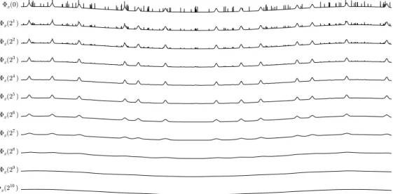
For practical purposes, the scale-space image is quantized across the scale dimension by computing the convolutions only for a finite number of scale parameters. More formally, for a given signalx, we fix a set of scale param-eters

S =_{2i _|0_≤i_≤σmax ∧i∈N}

and we compute Φx(σ) only for σ ∈ S where σmax is such that Φx(σ) is

approximately equal to the mean signal of x.

(35)

Φx(0)

Φx(21)

Φx(22)

Φx(23)

Φx(24)

Φx(25)

Φx(26)

Φx(27)

Φx(28)

Φx(29)

Φx(210)

Figure 3.2: Scale-space image of an artificially generated signal totalling 259 200 points.

As an example, Figure 3.2 shows the scale-space image of an artificially generated signal. The top plot represents the original signal, constructed by three components at different temporal scales: a slowly changing and slightly curved baseline, medium-term events (bumps) and short-term events (peaks). It is easy to visually verify that, by increasing the scale parameter, a larger amount of detail is removed. In particular, the peaks are smoothed out at scales greater thanσ = 24_{, and the bumps are smoothed out at scales greater}

than σ= 28_{, after which only the baseline remains.}

3.3.1 Relation to the Zero-Crossings of Derivatives

(36)

zero-3.4. MINIMUM DESCRIPTION LENGTH 27

0 1 2 4 8 16 32

Scale

0 200 400 600 800 1000 1200 1400 1600 1800

Number

of

zero-crossings

Figure 3.3: Relationship between the scale parameter and the number of zero-crossings of the first derivative of the signal shown in Figure 3.1.

crossing of the first derivative of the signal discussed in Figure 3.1.

3.4 Minimum Description Length

A recurring idea in this thesis is that learning and finding regularities in data can be seen as a form ofcompression. Compression is the act of representing some given data in the most compact way possible, such that its compressed representation has a lower number of bits than the original one [80]. The idea that the better we can compress a given data set, the more we can learn about it is a powerful one and it is formalized by the Minimum Description

Length principle.

The Minimum Description Length [34] is an information-theoretic model se-lection framework that selects the best model according to its ability to

compress the given data. In our context, the two-part MDL principle states

(37)

• L(M) is the length, in bits, of the description of the model,

• L(x _| M) is the length, in bits, of the description of the signal when encoded with the help of the modelM.

Given some data, MDL looks for a trade-off between the accuracy of a model and its complexity. Conceptually, MDL is a practical instantiation of the Oc-cam’s razor principle which states that, among several different hypotheses, the simplest is often also the best [91]. Moreover, MDL naturally protects against over-fitting as the principle takes into account the notion of model complexity and it discards models that are too complicated.

As we are dealing with unsupervised learning from time series data and we are interested in models that are as general as possible, the properties of the MDL framework makes it an ideal choice when designing model selection procedures.

In fact, prior work [42, 78, 88, 19, 10, 52] has already validated the effective-ness of the MDL approach when dealing with time series data and, through-out this thesis, we will further investigate its applicability to the analysis of sensor data.

3.4.1 Time Series Discretization

In order to use the MDL principle, we need to work with a quantized input signal and scale-space image. Because of this, we assume that the values

v of the input signal x (and of the scale-space components Φx(σ) for each

consideredσ) have been quantized to a finite number of symbols by employing the function defined below:

Q(v) =j v−min(x) max(x)₋min(x)l

k − ₂l

(38)

3.4. MINIMUM DESCRIPTION LENGTH 29

One question that might arise is if such a quantization removes meaning-ful information from the time series. In [42], the authors show that the effect of quantization is rather modest on several time series from various domains.

3.4.2 MDL Noise Filtering

In 3.2.3, we have shown how Gaussian convolution can be used to remove high-frequency components from a given signal and, thus, serve as a noise removal filter. We stressed, however, that the choice of the parameterσ, is a critical one and strictly depends on the characteristics of the data at hand. In this section, we use the Minimum Description Length principle to select the optimal σ given a time series, where by optimal we mean the one that retains the most characteristic information in the data.

Assume we are given a time series x of length n and, as we are using MDL, its values have been discretized to a fixed cardinality (in this example, 256 possible values) using the quantization functionQintroduced in above. In order to frame the problem from an MDL perspective, we first have to define what the possible models for x are. We consider the components of the scale-space Φx, quantized to different cardinalities, as models. In other

words, given a scale parameter σ and a cardinality c, we define a model for

xas Mσ,c =Q(Φx(σ), c), where Q is a quantization function.

(39)

0 200 400 600 800 1000 −1

0 1 2 3 4 5

0 200 400 600 800 1000

−1 0 1 2 3 4 5

0 200 400 600 800 1000

−1 0 1 2 3 4 5

Figure 3.4: Example of MDL-based noise filtering.

signal and the subtle vibrations iduced by the passing truck are retained. The bottom plot, finally, shows the optimal model (quantized) according to MDL. For this particular example, we consideredσ _{∈ {}2,22_,₂3_,₂4_,₂5_,₂6_}_and

the cardinality c_{∈ {}4,8,16,32,64,128,256_}. The optimal model is given by

σ= 23 _and _c_{= 8.}

(40)

Chapter 4 Identifying the Relevant

Temporal Scales

4.1 Introduction

When monitoring complex physical systems over time, one often finds mul-tiple phenomena in the data that work on different time scales. If one is interested in analyzing and modeling these individual phenomena, it is cru-cial to recognize these different scales and separate the data into its under-lying components. In this chapter, we present a method for extracting the time scales of various phenomena present in large time series. The method combines concepts from the signal processing domain with feature selection and the Minimum Description Length principle [34] which we introduced in Chapter 3.

We introduced the need for analyzing time series data at multiple time scales in Chapter 1 and we discussed in Chapter 2 how this is nicely demonstrated by the InfraWatch project.

In this project, we employ a range of sensors to measure the dynamic response of the Hollandse Brug, a large Dutch highway bridge to varying traffic and weather conditions. When viewing this data (see Fig. 4.1a), one can easily distinguish varioustransient eventsin the signal that occur on different time

(41)

scales. Most notable are the gradual change in strain over the course of the day (as a function of the outside temperature, which influences stiffness parameters of the concrete), a prolonged increase in strain caused by rush hour traffic congestion, and individual bumps in the signal due to cars and trucks traveling over the bridge. In order to understand the various changes in the sensor signal, one would benefit substantially from separating out the events at various scales. The main goal of the work described here is to do just that: we consider the temporal data as a series of superimposed effects at different time scales, establish at which scales events most often occur, and from this we extract the underlying signal components.

We approach the scale selection problem from a Minimum Description Length (MDL) perspective (see Section 3.4). The motivation for this is that we need a framework in which we can deal with a wide variety of representations for scale components. The MDL framework was shown to be sufficiently general to provide this flexibility by Hu et al. [42] for the problem of choosing the best model for a given signal. Our main assumption here is that separating the original signal into components at different time scales will simplify the shape of the individual components, making it easier to model them sepa-rately. Our results show that, indeed, these multiple models outperform (in terms of MDL score) a single model derived from the original signal. While introducing multiple models incurs the penalty of having to describe these multiple models, there are much fewer ‘exceptions’ to be described compared to the single model, yielding a lower overall description length. For instance, in the sensor data of Fig. 4.1a, cars are often passing in one direction while there is rush hour congestion in the opposite direction. Using multiple mod-els, this is modeled accurately, while a single model will easily ignore these events.

As we discussed in detail in Section 3.3, the analysis of time scales in time series data is often approached from ascale-spaceperspective, which involves convolution of the original signal with Gaussian kernels of increasing size [103] to remove information at smaller scales. By subtracting carefully selected components of the scale-space, we can effectively cut up the scale space intok

(42)

4.1. INTRODUCTION 33

0:00 1:00 2:00 3:00 4:00 5:00 6:00 7:00 8:00 9:00 10:00 11:00 12:00 13:00 14:00 15:00 16:00 17:00 18:00 19:00 20:00 21:00 22:00 23:00 24:00 Time

St

ra

in

(

µm

/m

)

(a) (b)

Figure 4.1: (a) One day of strain measurements from a large highway bridge in the Netherlands. The multiple external factors affecting the bridge are visible at different time scales. (b) A detail of plot (a) showing one of the peaks caused by passing vehicles.

collection of derived features, and the challenge we face in this chapter is how to select a subset of k features, such that the original signal is decomposed into a set of meaningful components at different scales.

Our approach applies the MDL philosophy to various aspects of modeling: choosing the appropriate scales at which to model the components, deter-mining the optimal number of components (while avoiding overfitting on overly specific details of the data), and deciding which class of models to apply to each individual component. For this last decision, we propose two classes of models representing the components respectively on the basis of a discretization and a segmentation scheme. For this last scheme, we allow three levels of complexity to approximate the segments: piecewise constant approximations, piecewise linear approximations, as well as quadratic ones. These options result in different trade-offs between model cost and accuracy, depending on the type of signal we are dealing with.

A useful side product of our approach is that it identifies a concise represen-tation of the original signal. This represenrepresen-tation is useful in itself: queries run on the decomposed signal may be answered more quickly than when run on the original data. Furthermore, the parameters of the encoding may indicate useful properties of the data as well.

(43)

the signal decompositions and use MDL to select the best subset of scales. Section 4.4 presents an empirical evaluation of our method on both real-world and artificial data. Section 4.5 links our method to related work. Finally, Section 4.6 states our main conclusions and ideas for future work.

4.2 Scale-Space Decomposition

In this section, we show how to manipulate the scale-space image to filter out the effects of transient events in a specific range of scales. This will lead to the definition of a signal decomposition scheme.

Along the scale dimension of the scale-space image, short-time transient events in the signal will be smoothed away sooner than longer ones. In other words, we can associate with each event a maximum scale σcut such

that, for σ > σcut, the transient event is no longer present in Φx(σcut). This

fact leads to the following two observations:

• Given a signal scale-space image Φx, the signal Φx(σ) is only affected

by the transient events at scales greater than σ. This is conceptually equivalent to alow-pass filter in signal processing.

• Given a signal scale-space image Φx and two scales σ1 < σ2, the signal

Φx(σ1)−Φx(σ2) is mostly affected by those transient events present in

the range of scales (σ1, σ2). This is similar to aband-pass filterin signal

processing.

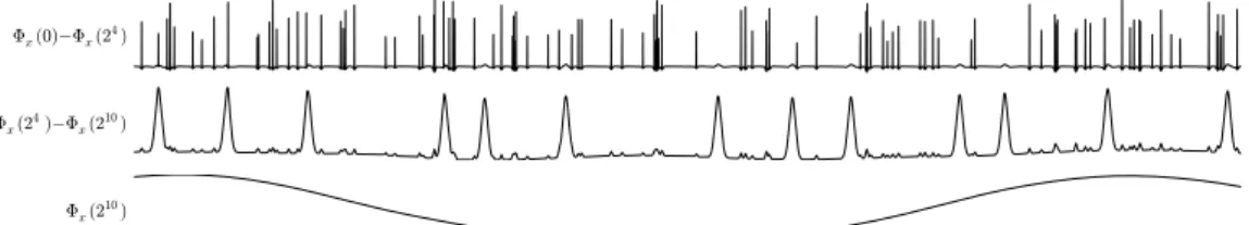
As an example, reconsider the signal x and its scale-space image Φx of

Fig-ure 3.2. FigFig-ure 4.2 shows (from top to bottom):

• the signal Φx(0)−Φx(24), which is the result of a high-pass filtering;

this feature represents the short-term events (peaks),

• the signal Φx(24)−Φx(210), which is the result of a band-pass filtering;

this feature represents the medium-term events (bumps),

• the signal Φx(210), which is the result of a low-pass filtering; this feature

(44)

4.2. SCALE-SPACE DECOMPOSITION 35

Φx(0)−Φx(24)

Φx(24)−Φx(210)

Φx(210)

Figure 4.2: Examples of signal decomposition obtained from the scale-space image in Figure 3.2.

Generalizing the example in Figure 4.2, we can define a decomposition scheme of a signalxby considering adjacent ranges of scales of the signal scale-space image. We formalize this idea below.

Definition (Scale-Space Decomposition). Given a signalxand a set of

k₋1 scale parameters C = _{σ1, . . . , σk−1} (called the cut-points set) such

that σ1 < . . . < σk−1, the scale decomposition of x is given by the set of

component signalsDx(C) = {x1, . . . ,xk}, defined as follows:

xi =



 

 

Φx(0)−Φx(σ1) if i= 1

Φx(σi−1)−Φx(σi) if 1< i < k

Φx(σk−1) if i=k

Note that for k components we requirek₋1 cut-points. This decomposition has several elegant properties:

• xk can be seen as the baseline of the signal, as obtained by a low-pass

filter;

• xi for 1≤i < k are signals as obtained by a band-pass filter, and can

be used to identify transient events;

• Pk

i=1xi =x, i.e., the original signal can be recovered from the

(45)

4.3 MDL Scale Decomposition Selection

Given an input signalx, the main computational challenge we face is twofold:

• find a good subset of cut-pointsCsuch that the resultingkcomponents of the decomposition Dx(C) optimally capture the effect of transient

events at different scales,

• select a representation for each component, according to its inherent complexity.

As stated before, the rationale behind the scale decomposition is that it is easier to model the effect of a single class of transient events at a given scale than to model the superimposition of many, interacting transient events at multiple scales. We thus need to trade off the added complexity of having to represent multiple components for the complexity of the representations themselves.

We approach this model selection problem by using the Minimum Description Length (MDL) principle introduced in Section 3.4. The possible candidate models depend on the scale decomposition Dx(C) considered1 and on the

representations used for its individual components. An ideal set of represen-tations would adapt to the specific features of every single component, result-ing in a concise summarization of the decomposition and, thus, of the signal. In order to apply the MDL principle, we need to define a model MDx(C) for

a given scale decomposition Dx(C) and, consequently, how to compute both L(MDx(C)) and L(x | MDx(C)). The latter term is the length in bits of the

information lost by the model, i.e., the residual signalx₋MDx(C).

As the MDL framework is only applicable to discrete data, we assume that the input signalxand the results of all the subsequent operations are discretized as discussed in Section 3.4.1. In the next sections, we introduce the proposed representation schemes for the components and define the bit complexity of the residual and the model selection procedure.

1_{Including the decomposition formed by zero cut-points (}_C₌

(46)

4.3. MDL SCALE DECOMPOSITION SELECTION 37

4.3.1 Component Representation Schemes

Within our general framework, many different approaches could be used for representing the components of a decomposition. In the next paragraphs we introduce two such methods.

Discretization-based representation

In some components of our data transient events always occur with similar amplitudes, mixed with long stretches of baseline values (see Figure 4.2). Hence, a desirable encoding could be one that captures this repetitiveness in the data by giving short codes to long stretches of the baseline and the commonly occurring amplitudes. Unfortunately, our original discretization is too fine-grained to capture regular occurrences of similar amplitudes. As a first representation, we hence propose to also consider more coarse-grained discretizations of the original range of values. We do this by discretizing each value v in a component to a value _bQ(v)/2i_c, where several values for i are considered for each component, typically i _{∈ {}2,4,6_}. By doing so, similar values will be grouped together in the same bin. The resulting sequence of integers is compacted further by performing run-length encoding, resulting in a string of (v, l) pairs, where l represents the number of times value v is repeated consecutively. This string is finally encoded using a Shannon-Fano or Huffman code (see Section 4.3.2).

As a simplified illustration of how the MDL principle helps here to identify components, consider data generated by the expression (67)n₍₀₁₎n ₍₄_n

inte-gers from the range _{0, . . . ,23₋₁_}_{), where we assume} _n _{and the range are}

fixed. In this data, each symbol occurs with the same frequency; we can en-code the time series hence with₋log₂(1/4)_·4_·n= 8n bits for the data, plus 8 lognbits for the dictionary of frequencies. Consider now the decomposition of the signal into two time series, 62n₀2n _{and (01)}2n_{. The first component,}

(47)

ampli-tudes, and 3 logn bits to identify the length of the one run-length (logn bit for identifying the number of run-lengths, in this case one, logn to identify the one run-length present, and lognto identify its frequency, from which the encoding with 0 bits follows). The second component can be encoded using 4n bits for the time series, as well as 8 lognbits for the dictionary. Assuming we also use 1 bit per component to identify the type of encoding used, this gives us an encoding in 4 + 19 logn+ 4n bits. Comparing this to 8n+ 8 logn

bits, forn _≥11 we will hence correctly identify the two components in this simplified data.

Segmentation-based representation

The main assumption on which we base this method is that a clear transient event can be accurately represented by a simple function, such as a poly-nomial of a bounded degree. Hence, if a signal contains a number of clear transient events, it should be possible to accurately represent this signal with a number of segments, each of which represented by a simple function. Given a component xi of lengthn, let

z(xi) = {t1, t2, . . . , tm}, 1< ti ≤n

be a set of indexes of the segment boundaries.

Let fit(xi[a : b], di) be the approximation of xi[a : b] obtained by fitting

a polynomial of degree di. Then, we represent each component xi with the

approximation ˆxi, such that:

ˆ

xi[0 :z1] =fit(xi[0 :z1], di)

ˆ

xi[zi :zi+1] =fit(xi[zi :zi+1], di), 1≤i < m

ˆ

xi[zm :n] =fit(xi[zm :n], di)

Note that approximation ˆxi is quantized again by reapplying the function Q

to each of its values.

For a given k-components scale decomposition Dx(C) and a fixed

(48)

4.3. MDL SCALE DECOMPOSITION SELECTION 39

of the model MDx(C), based on this representation scheme, as follows. Each

approximated component ˆxi consists of |z(xi)|+ 1 segments. For each

seg-ment, we need to represent its length and the di+ 1 coefficients of the fitted

polynomial. The length lsi of the longest segment in ˆxi is given by lsi = max(z1∪ {zi+1−zi |0< i≤m})

We therefore use log₂(lsi) bits to represent the segment lengths, while for the

coefficients of the polynomials we employ floating point numbers of fixed2 bit complexity c. The MDL model cost is thus defined as:

L(MDx(C)) =

k

X

i=1

(_|z(xi)|+ 1) (dlog2(lsi)e+c(di+ 1))

So far we assumed to have a set of boundaries z(xi), but we did not specify

how to compute them. A desirable property for our segmentation would be that a segmentation at a coarser scale does not contain more segments than a segmentation at a finer scale. The scale space theory assures that there are fewer zero-crossing of the derivatives of a signal at coarser scales [103]. In our segmentation, we use the zero-crossings of the first and second derivatives. More formally, we define the segmentation boundaries of a component xi to

be

z(xi) =

t_∈_R

dxi

dt (t) = 0

[

t _∈_R

d2_x

i

dt (t) = 0

.

Figure 4.3b shows an example of segmentation obtained as above using fitted polynomials of degree 1.

However, many other segmentation algorithms are known in the literature [48, 53] and all of them can be interchangeably employed in this context.

4.3.2 Residual Encoding

Given a model MDx(C), its residual r = x−

Pk

i=1xˆi, computed over the

components approximations, represents the information of x not captured

(49)

(a) (b)

Figure 4.3: Example of discretization-based encoding (a) and segmentation-based encoding with first degree polynomial approximations (the markers show the zero-crossings) (b).

by the model. Having already defined the model cost for the two proposed encoding schemes, we only still need to define L(x _| MDx(C)), i.e., a bit

complexity L(r) for the residual r.

Here, we exploit the fact that we operate in a quantized space; we encode each bin in the quantized space with a code that uses approximately ₋log(P(x)) bits, where P(x) is the frequency of the xth bin in our data. The main justification for this encoding is that we expect that the errors are normally distributed around 0. Hence, the bins in the discretization that reflect a low error will have the highest frequency of occurrences; we will give these the shortest codes. In practice, such codes can be obtained by means of Shannon-Fano coding or Huffman coding; as Hu et al. [42] we use Huffman coding in our experiments.

4.3.3 Model Selection

We can now define the MDL score that we are optimizing as follows:

Definition (MDL Score). Given a model MDx(C), its MDL score is

de-fined as:

L(MDx(C)) +L(r)

(50)

segmentation-4.4. EXPERIMENTS 41

based encoding the MDL score depends on the boundaries of the segments and the degrees of the polynomials in the representation. In both cases, also the cut-points of the considered decomposition affect the final score.

The simplest way to find the model that minimizes this score is to enu-merate, encode and compute the MDL score for every possible scale-space decomposition and all possible encoding parameters. As we shall now show, this brute-force approach is practically feasible.

The number of possible scale decompositions depends on the total number of cut-points sets we can build from the computed scale parameters in Φx.

We fix the maximum number of cut-points in a candidate set to some value

cmax. This also means that we limit our search to those scale decompositions

having cmax + 1 components or less. Moreover, given our wish to consider

only simple approximations of the signals, we can also assume a reasonably low limit dmax (in practice,dmax = 2) on the degree of the polynomials that

approximate the segments of each given component.

Computing the MDL score for each encoded scale decomposition, obtained by ranging over all the possible configurations of cut-points C1, . . . , Ck−1,

and all the possible configurations of polynomial degrees d1, . . . , dk, hence

requires calculating MDL scores for

cmax+1 X

k=2

|S_|

k₋1

dk_max

scale decompositions. This turns out to be a reasonable number in most practical cases we consider, and hence we use an exhaustive approach in our experiments.

4.4 Experiments

(51)

0 50000 100000 150000 200000 0.00

0.25 0.50

0 50000 100000 150000 200000

0.00 0.25 0.50

0 50000 100000 150000 200000

0.00 0.25 0.50

0 50000 100000 150000 200000

0.00 0.25 0.50

(a)

0 50000 100000 150000 200000

0.0 0.3 0.6

0 50000 100000 150000 200000

0.0 0.3 0.6

0 50000 100000 150000 200000

0.0 0.3 0.6

0 50000 100000 150000 200000

0.0 0.3 0.6

(b)

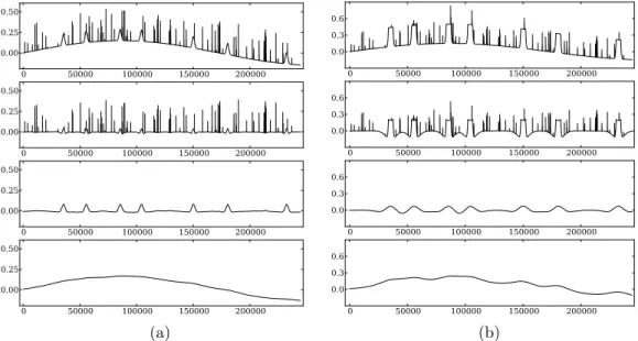
Figure 4.4: Signals (top) and top-ranked decompositions for the two artificial datasets.

tested it on a range of artificial datasets3 that mimic some of the multi-scale phenomena present in the bridge data. Our constructed data deliberately varies from easy, with clearly separated scales, to challenging with a variety of event shapes and sizes. All artificial datasets represent sensor data mea-sured at 1 Hz for a duration of three days (totaling 259,200 data points). The data was produced by combining three components at three distinct scales, resembling 1) individual events from vehicles, 2) traffic jams that last several tens of minutes, and 3) gradual change of the baseline, due to temperature changes of the bridge over the course of several days.

Artificial data

We start by considering one particular dataset in detail (see Figure 4.4a). This dataset was constructed by using Gaussian shapes for both the small and medium-scale events, and a sine wave of period 2.25 days at the largest

3_{The artificial datasets and the source code can be obtained by contacting the first}

(52)

4.4. EXPERIMENTS 43

scale. Medium events have a constant height, whereas small-scale events have a random height. We limited the search space to decompositions having a maximum of 4 components (3 cut-points). As can be seen in Figure 4.4a, our method was able to identify the fact that this data contains three impor-tant scales. Furthermore, the method correctly identified the two necessary cut-points, such that the three original components were reconstructed. The selected cut-points4 appear at scales 29 = 512 and 212 = 4096. When con-sidering the separated components in detail, some influence across the scale-boundaries is visible, for example where small effects of the ‘traffic jams’ appear among the small-scale events. These effects seem unavoidable, with the inherent limitations of the scale-space-based band-pass filtering and the discrete collection of scales we consider (powers of 2).

This optimal result has an MDL-score of 509,000 bits, being the sum of the model cost (L(M) = 75,072) and the error length (L(D _| M) = 433,928). The second-ranked result on this data, with cut-pointsC =_{211_,₂13_}_{, shows}

a similar result, however with slightly more pronounced cross-boundary ar-tifacts in the smallest scale, as is expected with a doubling of the lower cut-point. The MDL-score of this result is 64,896 + 450,487 = 515,383. The k = 1 case, which corresponds to compression of the original signal without any decomposition, appears at rank three, with an MDL-score of 44,640 + 471,271 = 515,911. This model obviously has a much lower model cost, due to having to represent only a single component, but this is com-pensated by the substantially higher error length, putting it below the scale-separated results. Ranks four and five represent two k = 2 results, where the former groups the small and medium scales together, and the latter the medium and large. All results in the top 10 relate to models that use poly-nomial representations (d_≤2).

Not all artificial datasets considered produced perfect results. In Figure 4.4b, we show an example of a dataset that includes ‘traffic jams’ that resemble more closely some of the phenomena in the actual sensor data. In many cases, traffic jams appear fairly rapidly, and then show an increased load on

4_{Note that our method returns the boundaries between scales, rather than the actual}

(53)

the bridge over a prolonged period. This is modeled in the data by medium-scale events that start and stop fairly rapidly, and remain constant in the meantime. The best result found, with cut-points C = _{212_,₂13_}_{, is shown}

in Figure 4.4b. This demonstrates that the proposed method is not able to properly separate the medium and low-scale events. In fact, even though the medium component does identify the location of the ‘traffic jams’, most of the rectangular nature is accounted for by the small scale. To some extent, this is understandable, as the start and end of the event could be considered high-frequency events with rapid changes in value. Therefore, parts of these events appear at a small scale, and the algorithm is mirroring this effect. In any case, the algorithmis able to identify the correct number of components, and is able to produce indications as to the location of the traffic jams. The top four results all show similar mixtures of scales, whereas the rank-five result groups the lowest two scales together. The k = 1 result appears at rank 14.

In order to better understand to what extent the proposed method is able to separate components at different scales, we carried out a more controlled experiment. We generated 11 different datasets constructed from 3 com-ponents. We fixed the scales of the short-term and long-term components respectively around σ= 23 _and _σ _{= 2}15_{, while the scale of the medium-term}

component varies from dataset to dataset in the range (24_{, . . . ,}₂14_{). The table}

below shows the number of components (k) of the top-ranked decomposition for the 11 datasets according to the scale parameter σ of the medium-term component.

σ 24 25 26 27 28 29 210 211 212 213 214

k 1 2 2 2 3 3 3 3 1 1 1

As the table suggests, the proposed method fails to identify the right number of components when the scales are too close to each other. However, when the scales are separated sufficiently (28 _≤ _σ _≤ ₂11_{), the right number of}

(54)

4.4. EXPERIMENTS 45

0 10 20 30

Figure 4.5: Signal (top) and top-ranked scale decomposition for the In-fraWatch data.

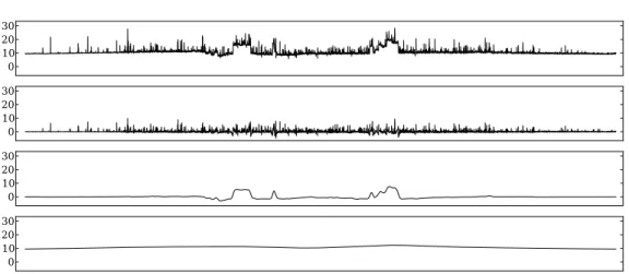
InfraWatch data

As anticipated by the motivating example in the introduction, we consider the strain measurements produced by a sensors attached to a large highway bridge in the Netherlands. For this purpose, we consider a time series con-sisting of 24 hours of strain measurements sampled at 1 Hz (totaling 86,400 data points). A plot of the data is shown in Figure 4.5 (topmost plot). We evaluated all the possible decompositions up to three components (two cut-points) allowing both the representation schemes we introduced. In the case of the discretization-based representations, we limit the possible cardinalities to 4, 16 and 64.

The top-ranked decomposition results in 3 components as shown in the last three plots in Figure 4.5. The selected cut-points appear at scales 26 _{= 64 and}

211 _{= 2048. All three components are represented with the}

discretization-based scheme, with a cardinality of respectively 4, 16, and 16 symbols. The decomposition has an MDL-score of 344,276, where L(M) = 19,457 and

L(D_|M) = 324,818. The found components accurately correspond to phys-ical events on the bridge. The first component, covering scales lower than 26_,

Mining sensor data from complex systems

Mining Sensor Data from

Complex Systems

Proefschrift

Ugo Vespier

Contents

Chapter 1

Introduction

1.1

Thesis Outline

Chapter 2

Sensor Data and Complex

Systems

2.1

Big Data

2.2

Sensor Networks and the Internet of Things

2.3

Multi-Scale nature of Complex Systems

2.4

SHM and InfraWatch

2.4.1

The InfraWatch project

Chapter 3

Preliminaries and

Background

3.1

Preliminaries

3.2

Convolution and Filtering

3.2.1

Convolution and LTI Systems

3.2.2

Discrete Convolution

3.2.3

Noise Filtering via Gaussian Smoothing

3.3

Scale-Space Image

3.3.1

Relation to the Zero-Crossings of Derivatives

3.4

Minimum Description Length

3.4.1

Time Series Discretization

3.4.2

MDL Noise Filtering

Chapter 4

Identifying the Relevant

Temporal Scales

4.1

Introduction

4.2

Scale-Space Decomposition

4.3

MDL Scale Decomposition Selection

4.3.1

Component Representation Schemes

4.3.2

Residual Encoding

4.3.3

Model Selection

4.4

Experiments