Efficient algorithms for detecting genetic interactions in genome-wide association study

(1)

Efficient Algorithms for Detecting Genetic Interactions in

Genome-Wide Association Study

Xiang Zhang

A dissertation submitted to the faculty of the University of North Carolina at Chapel Hill in partial fulfillment of the requirements for the degree of Doctor of Philosophy in the Depart-ment of Computer Science.

Chapel Hill 2011

Approved by: Wei Wang, Advisor

Fei Zou, Reader Leonard McMillan, Reader

(2)

(3)

Abstract

Xiang Zhang: Efficient Algorithms for Detecting Genetic Interactions in Genome-Wide Association Study.

(Under the direction of Wei Wang.)

(4)

List of Tables

1.1 An example dataset in genome-wide association study . . . 2

2.1 Possible groupings of phenotype values by the genotypes ofXiand(XiXj) . 12 2.2 Notations used in the bounds on∆Aand∆B . . . 18

2.3 Statistics of the SNP datasets . . . 26

2.4 Pruning effects on cardiovascular, metabolism and neurosensory datasets when finding critical valueFα . . . 30

2.5 Pruning effect on cardiovascular, metabolism and neurosensory datasets when findingFYk for all permutations . . . 32

2.6 Pruning effect when finding critical valueFαusing three synthetic phenotypes 33 3.1 Contingency tables for chi-square testing . . . 36

3.2 Notations used in the derivation of the upper bound . . . 43

4.1 Contingency tables . . . 59

4.2 Pruning effects of FastChi and COE using four different statistics . . . 70

5.1 An example dataset . . . 76

5.2 Contingency tables for single-locus tests T (Xi, Yk), T (Xj, Yk), genotype relation between(Xi, Xj), and two-locus testT (XiXj, Yk) . . . 77

5.3 Genotype difference between the connected SNPs in the minimum spanning tree shown in Figure 5.1 . . . 82

5.4 UpdatingOd2(X3X5)fromOd2(X3X2)for all permutations in a batch mode . 83 5.5 The tree weight and the proportion of the individuals pruned by TEAM on the human datasets . . . 90

(8)

(9)

List of Figures

1.1 Examples of associations between a phenotype and two different SNPs . . . . 3

2.1 An example of determining the critical value using permutation test . . . 15

2.2 The index arrayArray(X1)for efficient retrieval of the candidate SNP-pairs . 21 2.3 Performance comparison between FastANOVA and the brute-force approach when varying Type I error thresholds . . . 28

2.4 Performance comparison between FastANOVA and the brute-force approach when varying the number of SNPs . . . 28

2.5 Performance comparison between FastANOVA and the brute-force approach when varying the number of permutations . . . 29

2.6 Finding significant SNP-pairs (cardiovascular dataset) . . . 30

2.7 Finding significant SNP-pairs (metabolism dataset) . . . 31

2.8 Finding significant SNP-pairs (neurosensory dataset) . . . 31

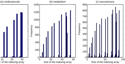
2.9 Histogram of the sizes of the indexing structures . . . 32

3.1 Pruning SNP-pairs inAP(Xi)using the upper bound . . . 45

3.2 AccessingArray(Xi)to retrieve the candidate SNP-pairs . . . 47

3.3 Distribution of the maximum chi-square test values of 1000 permutations . . 51

3.4 Performance comparisons between FastChi and the brute force approach un-der different settings. . . 53

3.5 Pruning effect of the upper bound . . . 54

3.6 Computational cost of each component of FastChi . . . 56

4.1 Convexity Example . . . 63

(10)

4.4 Indexing SNP-pairs . . . 66 4.5 Performance comparison of the brute force approach, FastChi, and COE Chi . 69 4.6 Performance comparison of the brute force approach, COE G, COE MI, and

COE T . . . 70 4.7 FastChi v.s. COE Chi . . . 71

5.1 The minimum spanning tree built on the SNPs in the example dataset shown in Table 5.1 . . . 82 5.2 Comparison between TEAM and the brute-force approach on human datasets

under various experimental settings . . . 89 5.3 Comparison between TEAM, COE, and the brute force approach on mouse

(11)

Chapter 1 Introduction

Genome-wide association study (GWAS) examines the genetic variants across the entire genome to identify genetic factors associated with observed phenotypes. It has been shown to be a promising design to locate the genetic factors causing phenotypic differences ( Saxena et al. (2007); The Wellcome Trust Case Control Consortium (2007)). Since most traits of interest are complex, finding gene-gene interaction has received increasing attention in recent years (Cordell (2009); Musani et al. (2007)).

1.1 Genome-Wide Association Study

(12)

SNPs Phenotype

X1 X2 X3 X4 X5 · · · X1000 Y

0 0 0 1 0 1 8

0 0 0 0 0 0 7

0 1 1 0 0 · · · 1 12

0 1 0 0 1 0 11

0 1 0 1 0 1 9

0 1 0 0 0 · · · 0 13

1 0 1 1 1 1 6

1 0 0 0 1 0 4

1 1 1 1 1 · · · 1 2

1 0 0 1 0 0 5

1 0 0 1 0 1 0

1 0 1 1 0 · · · 0 3

Table 1.1: An example dataset in genome-wide association study

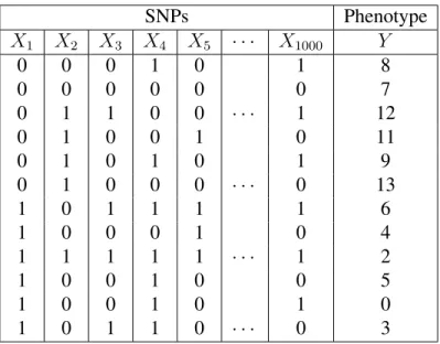
A phenotype is an observable trait or characteristic of an individual. Phenotypes can be either quantitative or binary. Examples of quantitative phenotypes are height and weight. These phenotypes can be represented by continuous variables. Binary phenotypes are usually studied in case-control studies. In such studies, the samples either have or do not have a certain disease. We can use{0,1}to indicate the disease status of an individual. Table 1.1 shows an example dataset consisting of 1000 SNPs{X1, X2,· · · , X1000}and a quantitative phenotype

Y for 12 individuals.

Genome-wide association studies (GWAS) find associations between SNPs and pheno-types across a set of individuals under study. More formally, letX = {X1, X2,· · · , XN}be the set of N SNPs for M individuals in the study, andY be the phenotype of interest. The goal of GWAS is to find SNPs inX, that are highly associated withY.

(13)

0 1

ph

en

oty

pe

va

lue

s

X₁ 4

8 12

(a) Strong association

0 1

ph

en

oty

pe

va

lue

s

X₁₀₀₀

4 8 12

(b) No association

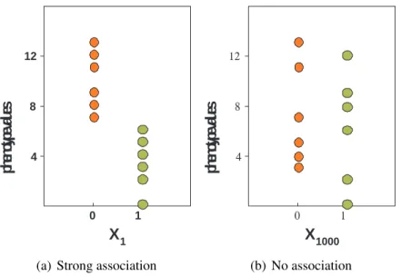
Figure 1.1: Examples of associations between a phenotype and two different SNPs

(14)

1.2 Epistasis Detection and Challenges

Many phenotypes of interest are complex in the sense that they are likely caused by the joint effects of multiple genes (Carlson et al. (2004); Segr et al. (2005)). In order to understand the underlying biological mechanisms of complex phenotype, one needs to consider the joint effect of multiple SNPs simultaneously. The interaction between genes is also referred to as

epistasis(Cordell (2009)). Although the idea of studying the association between phenotype and multiple SNPs is straightforward, the implementation is nontrivial. For a study with total

N SNPs, in order to find the association between n SNPs and the phenotype, a brute-force approach is to exhaustively enumerate all(N_n)possible SNP combinations and evaluate their associations with the phenotype. The computational burden imposed by this enormous search space often makes the complete genome-wide association study intractable.

The computational challenge of genome-wide association study is further compounded by another well-known statistical problem – the multiple testing problem (Miller (1981)). The multiple testing problem can be described as the potential increase in Type I error when statistical tests are performed multiple times. Letα be the Type I error for each independent test. Ifnindependent comparisons are performed, the experimental-wise errorα′ is given by

α′ = 1−(1−α)n.

For example, whenα = 0.05andn = 20,α′ = 1−0.9520 _{= 0}_.₆₄_{. We have 64% probability} to get at least one spurious result. Determining the statistical significance of the association between the phenotype and SNPs is crucial. Bonferroni correction based on the assumption that all n tests are independent is too conservative for the genome-wise association studies since SNPs are often correlated. Alternatively, a permutation procedure can be used and it is much preferred in association studies which automatically takes the correlation structure of SNPs into consideration.

(15)

Permutation test is used to estimate the null distribution (Churchill and Doerge (1994)). The idea is to randomly permute the phenotypeK times, whereK can be hundreds to thousands. The association analysis will be repeated in order to find the maximum test value for each permutated phenotype. Then the distribution of the K maximum test values is used as the approximated null distribution to assess the statistical significance of the findings from the original phenotype. Permutation test is usually very time-consuming since the test procedure needs to be performed in all permutations in order to find the maximum values.

Algorithm development to support these large scale analysis is still in its early stage. Most existing work focuses on studying associations between the phenotype and SNP-pairs and can only handle a small number of SNPs. Given a pair of SNPs, the phenotype values can be partitioned into at most four groups by the genotype of the SNP-pair, i.e., 00, 01, 10, and 11. Since each SNP has a distinct location on the genome, the association study of a phenotype and SNP-pairs is also calledtwo-locus association mapping. Important findings are appearing in the literature from studying the association between phenotypes and SNP-pairs (Saxena et al. (2007); Scuteri et al. (2007); Weedon et al. (2007)).

Although various statistical tests have been routinely applied to find association between SNP-pairs and phenotype, they are usually not performed in genome-wide scale. This is due to the fact that the search space of two-locus association mapping in genome-wide scale prohibits an exhaustive search. Suppose that the dataset consists ofN SNPs and the number of permutations isK. The total number of tests is KN(N−1)/2. Given a moderate number of SNPsN = 10,000and number of permutationsK = 1,000, the number of tests is around

(16)

1.3 Thesis Statement

Efficient exhaustive algorithms can be designed for two-locus epistasis detection in genome-wide association study. The proposed algorithms incorporate large permutation test for er-ror controlling. They guarantee to find the optimal solution. By applying effective pruning strategies, the computational cost of these algorithms can be dramatically reduced. Extensive experimental results demonstrate that the proposed algorithms are orders of magnitude faster than brute force alternatives.

1.4 Overview of the Developed Algorithms

This thesis presents a set of algorithms for two-locus epistasis detection. These programs use the permutation procedure for proper error control. They are exhaustive and accurate in the sense that no significant epistatic interactions between SNP-pairs are skipped. It has been theoretically proved and experimentally validated that these algorithms greatly speed up the epistasis test process. We give a brief overview of the designing principles of these programs here. All the algorithms utilize search space pruning to reduce the computational cost of epistatic test.

(17)

im-for all permutated data. Utilizing the upper bound and the indexing structure, FastANOVA only needs to perform the ANOVA test on a small number of candidate SNP-pairs without the risk of missing any significant pair.

The principal used in FastANOVA can also be applied to chi-square test. We can develop an upper bound for chi-square test, which is also expressed as the sum of two terms. The first term is based on the single-SNP chi-square test. The second term is based on the genotype of the SNP-pair and is independent of permutations. Based on this observation, we developed the FastChi algorithm (Zhang et al. (2009)).

The COE algorithm (Zhang et al. (2010)) takes the advantage of convex optimization. It can be shown that a wide range of statistical tests, such as chi-square test, likelihood ratio test (also known as G-test), and entropy-based tests are all convex functions of observed fre-quencies in contingency tables. Since the maximum value of a convex function is attained at the vertices of its convex domain, by constraining on the observed frequencies in the contin-gency tables, we can determine the domain of the convex function and get its maximum value. This maximum value is used as the upper bound on the test statistics to filter out insignificant SNP-pairs. COE is applicable to all tests that are convex.

(18)

1.5 Thesis Outline

The thesis is organized as follows:

• The FastANOVA algorithm is presented in Chapter 2. • The FastChi algorithm is presented in Chapter 3.

• The COE algorithm is presented in Chapter 4.

• The TEAM algorithm is presented in Chapter 5.

(19)

Chapter 2 The FastANOVA Algorithm

2.1 Introduction

Quantitative phenotype association study analyzes genetic variation across a population in or-der to find the genetic factors unor-derlying continuous phenotypes (such as height or weight). ANOVA (analysis of variance) test is one of the standard statistic methods and has been routinely used in quantitative phenotype association study (Pagano and Gauvreau (2000)). ANOVA test is used to determine whether the group means are significantly different. The total variance in the data is divided into within-group variance and between-group variance. If the between-group variance is sufficiently larger than the within-group variance, then the test concludes that there is significant phenotypic difference between the groups. Although ANOVA test has been a valuable tool to find association between SNP-pairs and quantitative phenotype, it is usually not performed at a genome-wide scale due to the enormous search space.

(20)

SNP-pairs. In fact, a large portion of the SNP-pairs are pruned without the need of performing the tests. FastANOVA establishes an upper bound on the two-locus ANOVA test. The upper bound is the sum of two terms: one based on the ANOVA test between phenotype and a single SNP, and the other based on the pair-wise SNP genotype and the ordered phenotype values. This formulation of the upper bound allows the algorithm to calculate the bound for a large number of SNPs together, which enables fast candidate retrieval. Moreover, the intermediate results for calculating the second term of the upper bound is independent of phenotype permutations. Hence they only need to be computed once and can be reused in all permutations. Applying this bound, FastANOVA is able to identify SNP-pairs with significant ANOVA test values using only a small fraction of the time required by performing ANOVA test on all SNP-pairs. The principles developed in FastANOVA are also applicable to the other statistical tests such as Chi-square test which is commonly used in case-control study where phenotypes are binary variables.

2.2 Related Work

The problem of genetic association study has attracted extensive research interests. In this sec-tion, we review the related work from a computational point of view. Please refer to (Doerge (2002); Hoh and Ott (2003); Balding (2006)) for excellent surveys of existing work.

(21)

of impurity in each iteration. These methods are not effective in detecting SNP combinations if there is little or no marginal effect.

Under the assumption that the number of SNPs is limited, e.g., from tens to hundreds, ex-haustive algorithms that explicitly enumerate all possible SNP combinations have been devel-oped. Combinatorial partitioning method (CPM) (Nelson et al. (2001)) is designed to identify multilocus genotypic partitions that predict quantitative trait variation. Given a small set of SNPs, CPM searches for the partitions of multilocus genotypes that are the most predictive in terms of phenotypic variability. Motivated by CPM, multifactorial dimension reduction (MDR) (Ritchie et al. (2001); Moore et al. (2006)) is designed for case/control studies. By pooling genotypes of multilocus into two groups at high disease risk and low disease risk, MDR reduces the genotype of multiple SNPs into one dimension. Among all possible com-binations, MDR selects the one that maximizes the case/control ratio of the high risk group. Since these methods explicitly enumerate all possible SNP combinations, they are not well adapted to genome-wide association studies.

To avoid exhaustively enumerating the search space, a common approach is to break the problem into two steps (Hoh et al. (2000); Evans et al. (2006)). First, a subset of important SNPs are selected. Second, within the selected subset, the association between SNPs and the phenotypes are searched. These methods are not complete since the SNPs with weak marginal effects may not be selected in the first step. Genetic algorithm (Carlborg et al. (2000); Nakamichi et al. (2001)) has been applied in finding SNP-pairs for quantitative phenotypes. These methods cannot guarantee to find the optimal solution.

(22)

(a) Grouping ofY byXi

Xi = 1 Xi = 0 groupA groupB

(b) Grouping ofY byXiXj

Xi = 1 Xi = 0

Xj = 1 groupa1 groupb1

Xj = 0 groupa2 groupb2

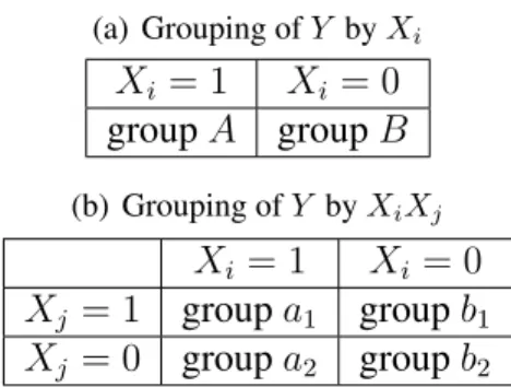
Table 2.1: Possible groupings of phenotype values by the genotypes ofXiand(XiXj)

association study. These methods are also not complete since some important SNPs may not be tagged.

2.3 The Problem

In this section, we formalize the problem of two-locus ANOVA test with permutation proce-dure. Let{X1, X2,· · · , XN}be the set of SNPs ofM individuals (Xi ∈ {0,1},1≤ i ≤N) andY ={y1, y2,· · · , yM}be the quantitative phenotype of interest, whereym(1≤m≤M) is the phenotype value of individualm.

For any SNPXi(1≤i≤N), we represent the F-statistic from the ANOVA test ofXiand

Y asF(Xi, Y). For any SNP-pair(XiXj), we represent the F-statistic from the ANOVA test of(XiXj)andY asF(XiXj, Y).

The basic idea of ANOVA test is to partition the total sum of squared deviationsSST into between-group sum of squared deviations SSB and within-group sum of squared deviations

SSW:

SST =SSB+SSW.

In the application of two-locus association study, Table 3.0(a) and Table 3.0(b) show the possible groupings of phenotype values by the genotypes ofXiand(XiXj)respectively. Let

(23)

(i.e., SNP-pair) analyses. Specifically, we have

SST(Xi, Y) =SSB(Xi, Y) +SSW(Xi, Y),

SST(XiXj, Y) =SSB(XiXj, Y) +SSW(XiXj, Y).

The F-statistics for ANOVA tests onXi and(XiXj)are:

F(Xi, Y) =

M −2 2−1 ×

SSB(Xi, Y)

SST(Xi, Y)−SSB(Xi, Y)

, (2.1)

F(XiXj, Y) =

M−g g−1 ×

SSB(XiXj, Y)

SST(XiXj, Y)−SSB(XiXj, Y)

, (2.2)

wheregin Equation (2.2) is the number of groups that the genotype of (XiXj)partitions the individuals into. Possible values ofg are 3 or 4, assuming all SNPs are distinct: If none of groupsA,B,a1,a2,b1,b2 is empty, theng = 4. If one of them is empty, theng = 3.

LetT = ∑

ym∈Y

ymbe the sum of all phenotype values. The total sum of squared deviations does not depend on the groupings of individuals:

SST(Xi, Y) = SST(XiXj, Y) =

∑

ym∈Y

y2_m−T

2

M.

Let Tgroup =

∑

ym∈group

ym be the sum of phenotype values in a specific group, andngroup be the number of individuals in that group. SSB(Xi, Y)andSSB(XiXj, Y)can be calculated as follows:

SSB(Xi, Y) =

T_A2 nA

+ T 2 B

nB −T2

M,

SSB(XiXj, Y) =

T2 a1

na1

+T 2 a2

na2

+ T 2 b1

nb1

+ T 2 b2

nb2

−T2

M.

Note that for any group ofA,B,a1,a2, b1, b2, if ngroup = 0, then

T2 group

ngroup

(24)

0.

The two-locus association mapping with permutation test is typically conducted in the following way (Pagano and Gauvreau (2000); Pesarin (2001); Mielke and Berry (2001)).

First, for every SNP-pair (XiXj)(1 ≤ i < j ≤ N), the ANOVA test is performed and

F(XiXj, Y)is recorded.

Second, a permutation test is performed to get a reference distribution in order to assess the statistical significance of previous findings. More specifically, a permutation Yk of Y is generated by sampling the phenotype Y without replacement. In other words, phenotype values are randomly assigned to individuals in the dataset with no single phenotype value being assigned to more than one individual. Let Y′ = {Y1, Y2,· · ·, YK} be the set of K permutations ofY. For each permutationYk ∈ Y′, letFYk represent the maximum F-statistic

value of all SNP-pairs, i.e.,

FYk = max{F(XiXj, Yk)|1≤i < j ≤N}.

The distribution of{FYk|Yk ∈Y′}is then used as the reference distribution for assessing the

statistical significance ofF(XiXj, Y)values found using the original phenotype Y: Given a Type I error thresholdα, thecritical valueFα is the αK-th largest value in{FYk|Yk ∈ Y

′_}_.

The SNP-pair(XiXj)whose F-statistic valueF(XiXj, Y)≥ Fα is considered as significant atα.

For example, Figure 2.1 shows the cumulative distribution of the maximum values for

K = 100permutations. Suppose thatα = 0.3, then Fα is the 30th largest value among the 100 maximum test values, which is 32 as shown in this example.

(25)

Maximum Test Values

Fr

eq

ue

nc

y

10 20 30 40

20 80

60

40 100

Critical Value

100 permutations Type I error = 0.3

F

30

32

Figure 2.1: An example of determining the critical value using permutation test

Problem (1): Given the Type I error threshold α, find the critical valueFα, which is the

αK-th largest value in{FYk|Yk∈Y′}.

Problem (2): Given the threshold Fα, find all significant SNP-pairs (XiXj) such that

F(XiXj, Y)≥Fα.

A brute force approach to these two problems is to enumerate all SNP-pairs and find their F-statistics. In Problem (1), for each permutation Yk ∈ Y, all SNP-pairs need to be enumerated in order to find the maximum valueFYk. In Problem (2), all SNP-pairs need to be

enumerated to see if their test values are above the thresholdFα. Computationally, Problem (1) is more challenging, since the permutation numberK can range form hundreds to thousands, which means the running time of finding the critical valueFα can be hundreds to thousands times longer than the running time of finding the significant SNP-pairs in Problem (2) using a brute-force search.

(26)

2.4 The Upper Bound

2.4.1 Updating F-Statistic

Since the total sum of squared deviations does not change, from the calculation ofF(Xi, Y) andF(XiXj, Y)(Equations (2.1) and (2.2)), we know that the relationship between these two tests only depends on the relationship between SSB(Xi, Y) and SSB(XiXj, Y). Next we show thatSSB(XiXj, Y)can be updated fromSSB(Xi, Y).

For groupsA,a1 anda2, let

∆A = T

2 a1

na1

+T 2 a2

na2

− TA2

nA

= na2T

2

a1 +na1T

2 a2

na1na2

−(Ta1 +Ta2)

2

na1 +na2

= (na2Ta1 −na1Ta2)

2

na1na2nA

= (nATa1 −na1TA)

2

na1(nA−na1)nA

.

Similarly, we have

∆B = T 2 b1

nb1

+T 2 b2

nb2

− TB2

nB

= (nBTb1 −nb1TB)

2

nb1(nB−nb1)nB

.

Thus,SSB(XiXj, Y)can be updated usingSSB(Xi, Y):

SSB(XiXj, Y) =SSB(Xi, Y) + ∆A+ ∆B. (2.3)

Note that if any one of {na1, na2, nA} is 0, then ∆A = 0. Similarly, if any one of

{nb1, nb2, nB}is 0, then∆B = 0.

(27)

2.4.2 Bounds on

∆

A

and

∆

B

Let{ym|ym ∈A} ={yA1, yA2,· · · , yA_nA}be the phenotype values in groupA. Without loss

of generality, assume that these phenotype values are arranged in ascending order, i.e.,

yA1 ≤yA2 ≤ · · · ≤yA_nA.

The derivative of∆Awith respect toTa1 is:

d∆A dTa1

= 2nA(nATa1 −na1TA)

na1(nA−na1)nA

.

Thus we have

∆Amonotonically

    

increases ifTa1 ≥

na1TA

nA

;

decreases ifTa1 ≤

na1TA

nA

.

We have the range ofTa1:

Ta1 ∈[la1, ua1] = [

na₁

∑

i=1

yAi,

nA

∑

i=nA−na₁+1

yAi].

The maximum value of∆Ais attained whenTa1 =la1 orTa1 =ua1, i.e.,

∆A≤ max{(nAla1 −na1TA)

2_,₍_n

Aua1 −na1TA)

2_}

na1(nA−na1)nA

. (2.4)

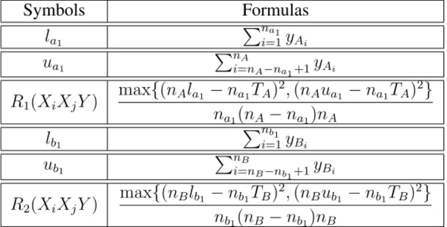
We useR1(XiXjY)to denote this upper bound.

Let{ym|ym ∈B}= {yB1, yB2,· · · , yB_nB}be the phenotype values in groupB. Without

loss of generality, assume that these phenotype values are arranged in ascending order, i.e.,

(28)

Symbols Formulas

la1

∑na₁

i=1yAi

ua1

∑nA

i=nA−na₁+1yAi

R1(XiXjY)

max{(nAla1 −na1TA)

2_,₍_n

Aua1 −na1TA)

2_}

na1(nA−na1)nA

lb1

∑nb1

i=1yBi

ub1

∑nB

i=nB−nb₁+1yBi

R2(XiXjY)

max{(nBlb1 −nb1TB)

2_,₍_n

Bub1 −nb1TB)

2_}

nb1(nB−nb1)nB

Table 2.2: Notations used in the bounds on∆Aand∆B

Similarly, we can derive the bound on∆B:

∆B ≤ max{(nBlb1 −nb1TB)

2_,₍_n

Bub1 −nb1TB)

2_}

nb1(nB−nb1)nB

. (2.5)

We use R2(XiXjY)to denote this upper bound. The symbols used in Inequalities (2.4) and (2.5) are summarized in Table 2.2.

From Equation (2.3), Inequalities (2.4) and (2.5), we have the overall upper bound on

SSB(XiXj, Y):

Theorem 2.4.1. (Upper bound ofSSB(XiXj, Y))

SSB(XiXj, Y)≤SSB(Xi, Y) +R1(XiXjY) +R2(XiXjY).

Property 2.4.2. The upper bound in Theorem 2.4.1 is tight.

The tightness of the bound is obvious from the derivation of the upper bound, since there exists some genotype of SNP-pair(XiXj)that makes the equality hold. For the same reason, we have the following property.

(29)

deviations, i.e.,

SSB(Xi, Y) +R1(XiXjY) +R2(XiXjY)≤SST(XiXj, Y).

2.5 The FastANOVA Algorithm

In this section, we show how our algorithm FastANOVA utilizes the upper bound in Theorem 2.4.1 to achieve efficient two-locus ANOVA testing. In Section 2.5.1, we describe the method for Problem (2) discussed in Section 2.3; that is, given a threshold Fα, we want to find all SNP-pairs whose F-statistics are greater than Fα. Then in Section 2.5.2, we discuss how FastANOVA performs in permutation procedure, i.e., the scenario of Problem (1) in Section 2.3.

2.5.1 A Single Phenotype

Given the thresholdFα, to find all SNP-pairs whose F-statistics are greater thanFα, a brute-force approach is to enumerate all SNP-pairs. To expedite this process, we employ the in-equality in Theorem 2.4.1 to prune SNP pairs that will have no chance to pass the significance thresholdFα. From Equation (2.2), we know that finding SNP-pairs(XiXj)whose F-statistics

F(XiXj, Y)≥Fα is equivalent to finding SNP-pairs satisfying

SSB(XiXj, Y)≥

SST(Xi, Y) M−g (g−1)Fα + 1

=θ.

Theorem 2.4.1 suggests that we only need to compute the F-statistics for the SNP-pairs that satisfy:

SSB(Xi, Y) +R1(XiXjY) +R2(XiXjY)≥θ.

We refer to these SNP-pairs ascandidateSNP-pairs.

(30)

all SNP-pairs is partitioned into non-overlapping groups such that each group has a common upper bound. For everyXi (1≤i≤N), letAP(Xi)be the set of SNP-pairs

AP(Xi) = {(XiXj)|i+ 1≤j ≤N}.

For all SNP-pairs inAP(Xi),nA, TA, nB, TB andSSB(Xi, Y)are constants. Moreover,la1,

ua1 are determined byna1, andlb1, ub1 are determined bynb1. Therefore, in the upper bound,

na1 and nb1 are the only variables that depend on Xj and may vary for different SNP-pairs

(XiXj)inAP(Xi).

Note thatna1 is the number of 1’s inXj whenXi takes value 1, andnb1 is the number of

1’s inXj whenXitakes value 0. It is easy to prove that switchingna1 andna2 does not change

the F-statistic value and the correctness of the upper bound. This is also true if we switchnb1

andnb2. Therefore, without loss of generality, we can always assume that na1 is the smaller

one between the number of 1’s and number of 0’s inXj whenXitakes value 1, andnb1 is the

smaller one between the number of 1’s and number of 0’s inXj whenXitakes value 0. For example, using the dataset showing in Table 1.1, for SNP-pair (XiX2),na = 1since the minimum of number of 1’s and 0’s in X2 when X1 = 1 is 1 (the number of 1’s), and

nb = 2since the minimum of number of 1’s and 0’s inX2 whenX1 = 0is 2 (the number of 0’s).

The following property specifies the values thatna1andnb1can take. The proof is

straight-forward and omitted here.

Property 2.5.1. If there arem1’s and(M −m)0’s inXi, then for any(XiXj) ∈ AP(Xi),

the possible values that na1 can take are{0,1,2,· · · ,⌊m/2⌋}. The possible values thatnb1

can take are{0,1,2,· · · ,⌊(M −m)/2⌋}.

(31)

n

_a1

n

_b1

0

2

0

2

1

3

1

3

(X₁X₂)

(X₁X₄)

(X_{1 .} )

. . .

(X_{1 .} )

(X₁X₃) (X₁X₅)

(X_{1 .} )

. . .

(X_{1 .} )

(3,1) (1,2)

(X_{1 .} )

. . . (X₁X₁₀₀₀)

(3,3)

Figure 2.2: The index arrayArray(X1)for efficient retrieval of the candidate SNP-pairs

Example 2.5.2. Using the example dataset shown in Table 1.1, we consider the SNP-pairs in

AP(X1), i.e., {(X1X2),(X1X3),(X1X4),(X1X5),· · · ,(X1X1000)}. There are 12

individu-als in the dataset. X1 contains 6 0’s and 6 1’s. Therefore, the possible values ofna1 andnb1

are {0,1,2,3}. Figure 3.2 shows the4×4array, Array(X1), whose entries represent the

possible values of (na1, nb1)for the SNP-pairs inAP(Xi). The entries in the same column

have the samena1 value. The entries in the same row have the samenb1 value. Thena1 value

of each column is noted beneath each column. Thenb1 value of each row is noted left to each

row. Each entry of the array is a pointer to the SNP-pairs having the corresponding(na1, nb1)

values. For example, for SNP-pair(X1X3), its(na1, nb1) = (3,1). Thus it is indexed by entry

(3,1).

Note that for a SNP-pair (XiXj) ∈ AP(Xi), na1 and na2 can be calculated faster than

performing the two-locus ANOVA test. To obtain na1 and na2, we only need to count the

(32)

Property 2.5.3. For any SNPXi, the maximum number of the entries inArray(Xi)is

(⌈M 4 ⌉+ 1)

2_.

The proof of Property 2.5.3 is straightforward and omitted here. In order to find candidate SNP-pairs, we scan all entries inArray(Xi)to calculate their upper bounds. Since the SNP-pairs indexed by the same entry share the same (na1, nb1) value, they have the same upper

bound.

Property 2.5.4. Given phenotype Y, for any SNP Xi, the SNP-pairs indexed by the same

entry inAP(Xi)have the same upper bound value.

For typical genome-wide association studies, the number of individualsM is much smaller than the number of SNPsN. From Property 2.5.3, there must be a group of SNP-pairs indexed by the same entry ofAP(Xi). In Example 2.5.2, there are in total 16 entries inArray(X1), and 999 SNP-pairs in AP(X1). Thus many SNP-pairs share the same (na1, nb1) value and

hence indexed by the same entry in Array(X1). Moreover, from Property 2.5.4, we can calculate the upper bound for the group of SNP-pairs indexed by the same entry together. It is these two key properties of the index structure that help to reduce the complexity of the algorithm. The additional cost for accessingArray(Xi)is minimal compared to performing ANOVA tests for all pairs(XiXj)∈AP(Xi)sinceM ≪N.

Algorithm 1 describes the FastANOVA algorithm for finding the SNP-pairs whose F-statistics are greater than the thresholdFα. The inputs of FastANOVA include the N SNPs, the phenotypeY and the critical valueFα. For eachXi, FastANOVA first indexes(XiXj)∈

(33)

Algorithm 1: FastANOVA (no phenotype permutation)

Input: SNPsX′ ={X1, X2,· · · , XN}, phenotypeY, and thresholdFα

Output: find the set of SNP-pairs

Result(Y) = {(XiXj)|F(XiXj, Y)≥Fα,1≤i < j ≤N}

foreveryXi ∈X′,do

1

index(XiXj)∈AP(Xi)byArray(Xi);

2

accessArray(Xi)to find the candidate SNP-pairs and store them inCand(Xi, Y);

3

forevery(XiXj)∈Cand(Xi, Y)do

4

ifF(XiXj, Y)≥Fα then

5

Result(Y)←(XiXj);

6

end

7

end

8

end

9

returnResult(Y).

10

2.5.2 Permutation Procedure

For multiple tests, permutation procedure is often used in genetic analysis for controlling family-wise error rate. For genome-wide association study, permutation is less commonly used because it often entails prohibitively long computation time. Our FastANOVA algorithm makes permutation procedure feasible in genome-wide association study.

Let Y′ = {Y1, Y2,· · · , YK} beK permutations of the phenotype Y. Following the idea discussed in Section 2.5.1, the upper bound in Theorem 2.4.1 can be easily incorporated in the algorithm to handle the permutations.

Property 2.5.5. For every SNP Xi, the indexing structure Array(Xi)is independent of the

permuted phenotypes inY′.

The correctness of this property relies on the fact that, for any (XiXj) ∈ AP(Xi), na1

andnb1 only depend on the genotype of the SNP-pair and thus remain constant for different

phenotype permutations. Therefore, for eachXi, once we buildArray(Xi), it can be reused in all permutations.

(34)

Algorithm 2: FastANOVA (for permutation test)

Input: SNPsX′ ={X1, X2,· · · , XN}, phenotype permutations

Y′ ={Y1, Y2,· · · , YK}, and the Type I errorα

Output: find the critical valueFα

T list←αK dummy phenotype permutations with F-statistics 0 ;

1

Fα = 0;

2

foreveryXi ∈X′,do

3

index(XiXj)∈AP(Xi)byArray(Xi);

4

foreveryYk ∈Y′,do

5

accessArray(Xi)to find the candidate SNP-pairs and store them in

6

Cand(Xi, Yk);

forevery(XiXj)∈Cand(Xi, Yk)do

7

ifF(XiXj, Yk)≥Fαthen

8

updateT list;

9

Fα = the smallest test value inT list;

10

end

11

end

12

end

13

end

14

returnFα.

15

is to find the critical value Fα, which is the αK-th largest value in {FYk|Yk ∈ Y

′_}_{. Recall}

that FYk is the maximum F-statistic value for phenotype Yk. We use T list to keep the αK

phenotype permutations having the largest F-statistics found by the algorithm so far. Initially,

T listcontainsαKdummy phenotype permutations with test values 0. The smallest F-statistic value in T list, initially 0, is used as the threshold to prune the SNP-pairs. For each Xi, FastANOVA first indexes (XiXj) ∈ AP(Xi) using Array(Xi). Then it finds the set of candidate SNP-pairsCand(Xi, Yk)by accessingArray(Xi)for every phenotype permutation

(35)

2.5.3 Complexity Analysis

In this section, we study the time and space complexities of the FastANOVA algorithm for permutation test. The complexity for a single phenotype can be analyzed in a similar way.

Time complexity: For eachXi, FastANOVA needs to index(XiXj)inAP(Xi). The com-plexity to build the indexing structure for all SNPs isO(N(N−1)M/2). The worst case for ac-cessing allArray(Xi)for all permutations isO(N×K×(⌈M₄ ⌉+1)2) = O(N KM2). LetC =

∑

i,k|Cand(Xi, Yk)|represent the total number of candidates. The overall time complexity of FastANOVA is thusO(N(N−1)M/2)+O(N K×(⌈M₄⌉+1)2)+O(∑_i,k|Cand(Xi, Yk)|M) =

O(N2_M₊_{N KM}2₊_CM₎_{. The experimental results show that the overhead of building the} indexing structures and accessing them for candidate retrieval are negligible when large per-mutation tests are needed. The time complexity of the brute-force approach isO(KN(N −

1)M/2) = O(KN2_M₎_{. Note that in a typical genotype-phenotype association study, the} number of SNPs N is much lager than the number of individuals M. Therefore, when the number of permutations K is large, e.g. thousands, the complexity of FastANOVA is much less than the complexity of the brute force approach.

Space complexity: The total number of variables in the dataset, including the SNPs and the phenotype permutations, is N +K. The maximum space of the indexing structure

Array(Xi)isO((⌈M₄⌉+ 1)2+N). Note that for each SNPXi, FastANOVA only needs to ac-cess one indexing structure,Array(Xi), for all permutations. Once the evaluation process for

Xi is done for all permutations,Array(Xi)can be cleared from the memory. Therefore, the space complexity of FastANOVA isO((N+K)M) +O((⌈M₄ ⌉+ 1)2+N) =O((N+K)M)

sinceM ≪N. The space complexity is linear to the dataset size.

2.6 Experimental Results

(36)

cardiovascular metabolism neurosensory

# individuals 19 26 34

# SNPs 14,513 43,856 66,006

Table 2.3: Statistics of the SNP datasets

the brute-force approach under various experimental settings, (2) the punning effect of the upper bound, and (3) the relative computational cost of each component of FastANOVA. Fas-tANOVA is implemented in C++. The experiments are performed on a 2.4 GHz PC with 1G memory running WindowsXP system.

Dataset: The SNP dataset used for the experiments is extracted from a set of combined SNPs from the 140k Broad/MIT mouse dataset (http : //www.broad.mit.edu/) and 10k GNF mouse dataset (http : //www.gnf.org/). This merged dataset has 156,525 SNPs for 71 individuals. The missing values in the dataset are imputed using NPUTE (Roberts et al. (2007)). We use both real phenotypes and synthetic phenotypes in our experiments. The real phenotype data is available from the Jackson Laboratory (http://www.jax.org/).

2.6.1 Real Phenotypes

We use three real phenotypes in our experiments: cardiovascular (blood pressure), metabolism (water intake), and neurosensory (acoustic startle response). Table 2.3 shows the statistics of the genotype datasets corresponding to the three phenotypes. The number of SNPs in the table indicates the number of unique SNPs in each genotype dataset.

We first show the results on finding the critical value Fα, which is more time-consuming than finding the significance SNP-pairs given the critical valueFαfor a single phenotype.

Finding critical valueFα

(37)

time-order to show the performance comparisons. The default setting is as follows: The Type I error thresholdα = 0.01. The number of permutations is 100. The number of SNP is 10,000 for the two larger datasets of metabolism and neurosensory, and 2,900 for the cardiovascular SNP dataset. These experimental settings are chosen to demonstrate the performance gain and enhanced scalability offered by FastANOVA over the brute-force implementation. Fas-tANOVA can handle much larger SNP panels and larger number of permutation tests. The performance of FastANOVA is expected to follow the same trends presented in the remainder of this section.

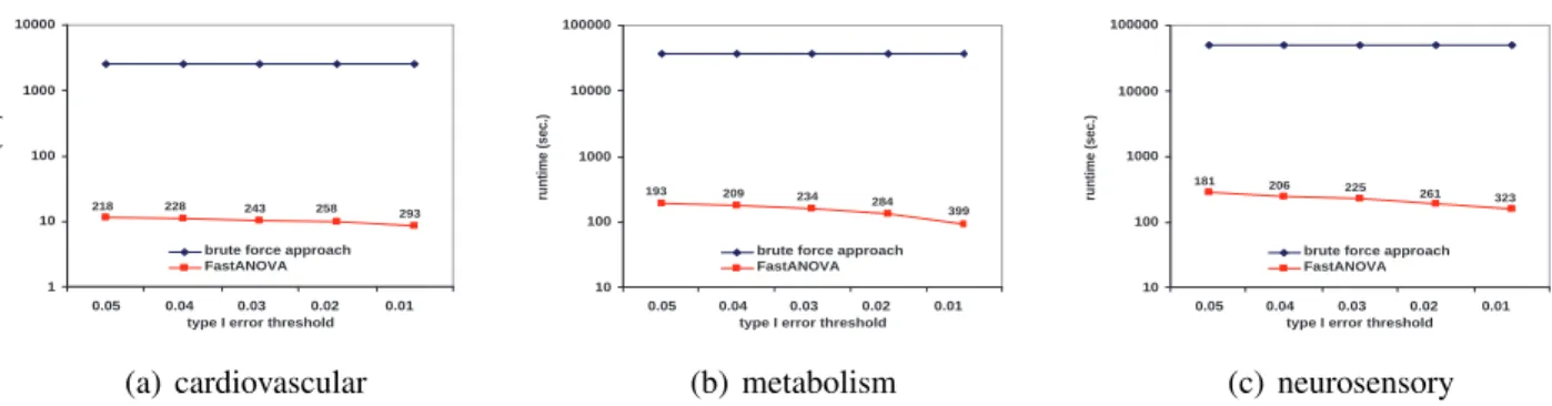
Figures 2.3, 2.4, and 2.5 show the running time comparison of FastANOVA and the brute-force approach on the three genotype phenotype datasets using different settings. The y-axis is in logarithm scale. The numbers above the runtime line of FastANOVA indicate the ratio of the runtimes of the brute-force approach over FastANOVA. We terminate the programs that have run over 72 hours without completion.

Figure 2.3 shows the runtime comparison when varying the Type I error thresholds. For each dataset, the runtime of the brute-force approach does not change over different Type I error thresholds. The runtime of FastANOVA decreases as the threshold decreases. Fas-tANOVA offers 218 fold speedup when α = 0.05and 293 fold speedup whenα = 0.01on cardiovascular dataset. We can also observe a similar two-orders-of-magnitude speedup in the metabolism and neurosensory datasets. This is consistent with the pruning effect of the upper bound, which will be presented later in this section. In general, the lower the Type I error threshold, the more powerful the pruning effect, hence the faster the algorithm.

(38)

1 10 100 1000 10000

0.05 0.04 0.03 0.02 0.01 type I error threshold

runtime (sec.)

brute force approach FastANOVA

218 228 243 258 293

(a) cardiovascular 10 100 1000 10000 100000

runtime (sec.)

brute force approach FastANOVA 399 284 234 209 193 (b) metabolism 10 100 1000 10000 100000

runtime (sec.)

brute force approach FastANOVA 323 261 225 206 181 (c) neurosensory

Figure 2.3: Performance comparison between FastANOVA and the brute-force approach when varying Type I error thresholds

1 10 100 1000 10000 100000

2.9k 5.8k 8.7k 11.6k 14.5k number of SNPs

runtime (sec.)

brute force approach FastANOVA 293 849 675 609 471 (a) cardiovascular 10 100 1000 10000 100000 1000000

10k 18k 26k 34k 42k

number of SNPs

runtime (sec.)

brute force approach FastANOVA 718 630 399 (b) metabolism 10 100 1000 10000 100000 1000000

10k 24k 38k 52k 66k

number of SNPs

runtime (sec.)

brute force approach FastANOVA 526

323

(c) neurosensory

Figure 2.4: Performance comparison between FastANOVA and the brute-force approach when varying the number of SNPs

performance gain of FastANOVA is even higher for larger SNP datasets.

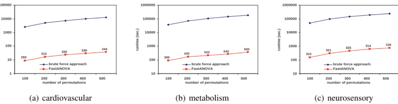
Figure 2.5 shows the runtime comparison when the number of phenotype permutations changes. The runtime of the brute-force approach is linear with respect to the number of permutations. FastANOVA is consistently two orders of magnitude faster than the brute-force approach. The performance gap increases as the number of permutations increases.

(39)

1 10 100 1000 10000 100000

100 200 300 400 500

number of permutations

runtime (sec.)

brute force approach FastANOVA 344 339 326 313 293 (a) cardiovascular 10 100 1000 10000 100000 1000000

100 200 300 400 500

runtime (sec.)

brute force approach FastANOVA 505 540 522 435 399 (b) metabolism 10 100 1000 10000 100000 1000000

100 200 300 400 500

runtime (sec.)

brute force approach FastANOVA 328 314 325 321 323 (c) neurosensory

Figure 2.5: Performance comparison between FastANOVA and the brute-force approach when varying the number of permutations

also increases. This is because, with more SNPs, the dynamic threshold used to prune the search space becomes higher. Hence a larger portion of SNPs are pruned. This is consistent with results shown in Figure 2.4. Note that from Table 2.4 we observe that the pruning ratio tends to remain steady when the number of permutations changes. However, we observe that the runtime ratio increases as the number of permutations increases. The reason for these two different trends will become clear after we show the results on the computational cost of each component of FastANOVA in the next subsection.

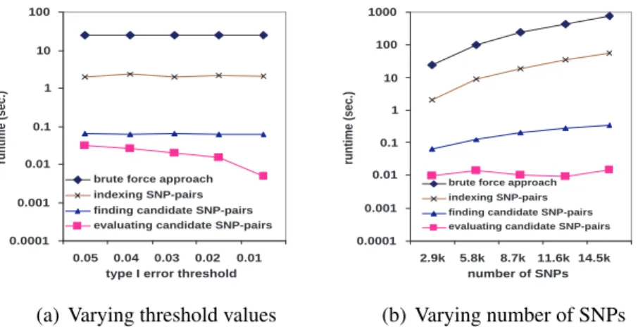
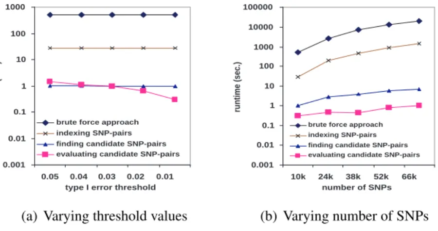
Finding significant SNP-pairs

In this subsection, we study the comparison between FastANOVA and the brute-force ap-proach in finding significant SNP-pairs given a critical valueFα. Only the original phenotype (without permutations) is used in this procedure. We examine the detailed computation cost of each component of the FastANOVA algorithm. FastANOVA has three major components: building the indexing structure Array(Xi) for every SNPXi, accessing Array(Xi) to find the candidate SNP-pairs, and performing ANOVA tests on these candidates.

(40)

cardiovascular metabolism neurosensory 0.05 99.881% 99.724% 99.701%

0.04 99.907% 99.758% 99.751%

α 0.03 99.928% 99.797% 99.792%

0.02 99.949% 99.877% 99.853%

0.01 99.974% 99.929% 99.911%

1st 99.974% 99.929% 99.911%

2nd 99.991% 99.985% 99.979%

# SNPs 3rd 99.996% 99.996% 99.997%

4th 99.998% 99.996% 99.997%

5th 99.998% 99.993% 99.998%

100 99.974% 99.929% 99.911%

200 99.966% 99.935% 99.917%

# Perm. 300 99.977% 99.962% 99.919%

400 99.977% 99.961% 99.914%

500 99.974% 99.953% 99.907%

Table 2.4: Pruning effects on cardiovascular, metabolism and neurosensory datasets when finding critical valueFα

0.0001 0.001 0.01 0.1 1 10 100

0.05 0.04 0.03 0.02 0.01

type I error threshold

runtime (sec.)

brute force approach indexing SNP-pairs finding candidate SNP-pairs evaluating candidate SNP-pairs

(a) Varying threshold values

0.0001 0.001 0.01 0.1 1 10 100 1000

2.9k 5.8k 8.7k 11.6k 14.5k

number of SNPs

runtime (sec.)

(b) Varying number of SNPs

Figure 2.6: Finding significant SNP-pairs (cardiovascular dataset)

(41)

0.001 0.01 0.1 1 10 100 1000

0.05 0.04 0.03 0.02 0.01

runtime (sec.)

0.001 0.01 0.1 1 10 100 1000 10000

10k 18k 26k 34k 42k

number of SNPs

runtime (sec.)

Figure 2.7: Finding significant SNP-pairs (metabolism dataset)

0.001 0.01 0.1 1 10 100 1000

0.05 0.04 0.03 0.02 0.01

runtime (sec.)

0.001 0.01 0.1 1 10 100 1000 10000 100000

10k 24k 38k 52k 66k

number of SNPs

runtime (sec.)

Figure 2.8: Finding significant SNP-pairs (neurosensory dataset)

(42)

10 20 30 Size of the indexing array

(a) cardiovascular

0 20 40 60

0 200 400 600 800 1000 1200 1400

Size of the indexing array

Frequency

(b) metabolism

0 50 100

0 100 200 300 400 500 600 700 800 900

Size of the indexing array

Frequency

(c) neurosensory

Figure 2.9: Histogram of the sizes of the indexing structures cardiovascular metabolism neurosensory

97.865% 97.844% 98.061%

Table 2.5: Pruning effect on cardiovascular, metabolism and neurosensory datasets when find-ingFYk for all permutations

Figure 2.9 shows the histogram of the sizes of the indexing structures for the three datasets. From Property 2.5.3, the maximum sizes of the indexing structures are 36 for the cardiovas-cular dataset, 64 for the metabolism dataset, and 100 for the neurosensory dataset. It is clear from the figure that the actual sizes of the indexing structures are much smaller than the max-imum sizes.

FindingFYk for all permutations

Sometimes users may be interested in finding FYk values of all phenotype permutations. In

this way, the users can get the critical valueFα for any Type I error thresholdαranging from 0 to 1, without re-running the permutation tests for different thresholds. Recall that, given a set of phenotype permutations Y′ = {Y1, Y2,· · · , YK}, FYk = max{F(XiXj, Yk)|1 ≤ i <

j ≤ N}is the maximum F-statistic value for permutationYk. Fα is the αK-th largest value in{FYk|Yk ∈ Y

(43)

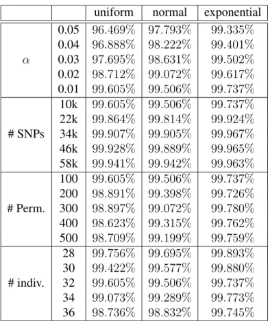
uniform normal exponential 0.05 96.469% 97.793% 99.335%

0.04 96.888% 98.222% 99.401%

α 0.03 97.695% 98.631% 99.502%

0.02 98.712% 99.072% 99.617%

0.01 99.605% 99.506% 99.737%

10k 99.605% 99.506% 99.737%

22k 99.864% 99.814% 99.924%

# SNPs 34k 99.907% 99.905% 99.967%

46k 99.928% 99.889% 99.965%

58k 99.941% 99.942% 99.963%

100 99.605% 99.506% 99.737%

200 98.891% 99.398% 99.726%

# Perm. 300 98.897% 99.072% 99.780%

400 98.623% 99.315% 99.762%

500 98.709% 99.199% 99.759%

28 99.756% 99.695% 99.893%

30 99.422% 99.577% 99.880%

# indiv. 32 99.605% 99.506% 99.737%

34 99.073% 99.289% 99.773%

36 98.736% 98.832% 99.745%

Table 2.6: Pruning effect when finding critical valueFα using three synthetic phenotypes

permutationYk, the dynamic threshold used to prune the search space is the largest F-statistic value ofYk identified by the algorithm so far.

Table 2.5 shows the pruning ratio of applying the upper bound to the three real phenotype datasets. The experimental setting is the same as the default setting before. As expected, the pruning ratios are slightly lower than those in Table 2.4, where smaller Type I error thresholds are used to prune the search space. However, the pruning ratios on all three datasets are still above 97%. Moreover, finding allFYk provides the advantage that we can get theFα values

for all possibleαvalues instead of just for a specific one.

2.6.2 Synthetic Phenotypes

(44)

exponential distribution. Our purpose is to study the pruning effect of the upper bound under different phenotype distributions. The default setting of the experiments in this subsection is as follows: #individuals = 32, #SNPs=10,000, #permutations=100, α = 0.01. There are 60,970 unique SNPs for these 32 individuals.

Table 2.6 shows the pruning ratio of FastANOVA under different settings using permuta-tion test. In this table, we also include the pruning ratio when the number of individuals varies. We observe that the pruning effects are similar to that of real phenotypes, which indicates that the upper bound pruning is effective and insensitive to different phenotype distributions.

2.7 Conclusion

The large number of available SNPs poses great computational challenge to the genome-wide association study. To assess the significance of the findings, permutation test is usually required. These factors make the association study a very time-consuming process. Thus tools that can improve the efficiency of the association study are in demand.

(45)

Chapter 3 The FastChi Algorithm

3.1 Introduction

As our initial attempt to develop scalable algorithms for genome-wide association study, Fas-tANOVA is specifically designed for the ANOVA test on quantitative phenotypes. Another category of phenotypes is generated in case-control study, where the phenotypes are binary variables representing disease/non-disease individuals. Chi-square test is one of the most commonly used statistics in binary phenotype association study. We can extend the principles in FastANOVA for efficient two-locus chi-square test (Zhang et al. (2009)). The general idea of FastChi is similar to that of FastANOVA, i.e., re-formulating the chi-square test statistic to establish an upper bound of two-locus chi-square test, and indexing the SNP-pairs according to their genotypes in order to effectively prune the search space and reuse redundant compu-tations. In this chapter, we introduce the FastChi algorithm.

(46)

(a) Contingency table forχ2(Xi, Y)

Xi = 0 Xi = 1 Total

Y = 0 eventA eventB Y = 1 eventC eventD

Total M

(b) Contingency table forχ2(XiXj, Y)

Xi = 0 Xi = 1 Total

Xj = 0 Xj = 1 Xj = 0 Xj = 1

Y = 0 eventa1 eventa2 eventb1 eventb2

Y = 1 eventc1 eventc2 eventd1 eventd2

Total M

Table 3.1: Contingency tables for chi-square testing

test. Consequently, FastChi is able to identify SNP pairs with significant chi-square values for a given phenotype using only a small fraction of the time required by performing two-locus chi-square test on all SNP pairs.

3.2 The Problem

Let {X1, X2,· · · , XN} be the set of all biallelic SNPs , andY be the binary phenotype of interest (e.g., disease or non-disease). We adopt the convention of using 0 to represent majority allele and 1 to represent minority allele, and use 0 for non-disease and 1 for disease. For any SNP Xi (1 ≤ i ≤ N), we represent the chi-square test value of Xi and Y as χ2(Xi, Y). For any SNP-pairXi andXj, we use χ2(XiXj, Y)to represent the chi-square test value for the combined effect of (XiXj) with phenotype Y. Table 3.0(a) and 3.0(b) show example contingency tables for calculatingχ2₍_X

i, Y)andχ2(XiXj, Y)whenXi,Xj andY are binary variables.

We formalize the problem as follows. Given a set ofN biallelic SNPs{X1, X2,· · · , XN} and a binary phenotypeY for a set ofM individuals. LetY′ ={Y1, Y2,· · ·, YK}be the set of

(47)

SNP-pairs(XiXj)such that

χ2(XiXj, Y)≥θ.

(2) In the case where there are multiple phenotype permutations: for each Yk ∈ Y′, find all SNP-pairs(XiXj)such that

χ2(XiXj, Yk)≥θ,(1≤k ≤K).

Note that ifY′ = {Y}then cases (1) and (2) are the same. Case (1) is actually a special case of (2). Our problem formalization can also be applied in other problem settings. For example, it is easy to modify this problem definition as finding the top-kSNP-pairs that have the largest chi-square test values among all SNP-pairs. In this scenario,θwould be a dynamic value, i.e., thek-th largest chi-square test value identified by the algorithm so far.

3.3 The Upper Bound

3.3.1 Updating Chi-square Statistic

In this section, we show that for any two SNPs,XiandXj,χ2(XiXj, Y)can be derived from

χ2₍_X

i, Y). The results in this section provide the foundation for developing the upper bound ofχ2₍_X

iXj, Y)which will be presented in Section 3.3.2.

LetA, B, C, D, a1, a2, b1, b2, c1, c2, d1, d2represent the events as shown in Table 3.0(a) and Table 3.0(b). LetEevent andOevent denote the expected value and observed value of certain event.χ2(Xi, Y)andχ2(XiXj, Y)can be calculated as follows:

χ2(Xi, Y) =

∑

event∈{A,B,C,D}

(Oevent−Eevent)2

Eevent ,

χ2(XiXj, Y) =

∑

event∈{a1,a2,b1,b2,c1,c2,d1,d2}

(Oevent−Eevent)2

(48)

For eventA, its corresponding component inχ2₍_X

i, Y)calculation is

(OA−EA)2

EA

.

For eventsa1 anda2, their corresponding component inχ2(XiXj, Y)calculation is

(Oa1 −Ea1)

2

Ea1

+(Oa2 −Ea2)

2

Ea2

.

Note that OA = Oa1 +Oa2, and EA = Ea1 +Ea2. The difference between these two

components is

∆A =

(Oa1 −Ea1)

2

Ea1

+(Oa2 −Ea2)

2

Ea2

− (OA−EA)2

EA

= M(Oa1Oc2 −Oa2Oc1)

2

(OA+OB)(OA+OC)(Oa1 +Oc1)(Oa2 +Oc2)

.

Similarly, for eventsC,c1 andc2, we have

∆C =

(Oc1 −Ec1)

2

Ec1

+(Oc2 −Ec2)

2

Ec2

− (OC −EC)2

EC

= M(Oc1Oa2 −Oc2Oa1)

2

(OC +OD)(OA+OC)(Oc1 +Oa1)(Oc2 +Oa2)

.

Adding∆Aand∆C together, we have∆A+ ∆C

= M

2₍_O

a1Oc2−Oa2Oc1)

2

(OA+OB)(OA+OC)(OC +OD)(Oa1 +Oc1)(Oa2 +Oc2)

.

Let

T1 =

M2

(OA+OB)(OA+OC)(OC +OD)

Efficient algorithms for detecting genetic interactions in genome-wide association study