Kontsevich Model
Johannes BRANAHL, Alexander HOCK and Raimar WULKENHAAR
Mathematisches Institut der WWU, Einsteinstr. 62, 48149 M¨unster, Germany
E-mail: j [email protected],a [email protected],[email protected] URL: http://www.uni-muenster.de/MathPhys/
Dedicated to Dirk Kreimer on the occasion of his 60th birthday
Abstract. The analogue of Kontsevich’s matrix Airy function, with the cubic potential Tr(Φ3) replaced by a quartic term Tr(Φ4), provides a toy model for quantum field theory in which all correlation functions can be computed exactly and explicitly. In this paper we show that distinguished polynomials of correlation functions, themselves given by quickly growing series of Feynman ribbon graphs, sum up to much simpler and highly structured expressions. These expressions are deeply connected with meromorphic forms conjectured to obey blobbed topological recursion. Moreover, we show how the exact solutions permit to explore critical phenomena in the Quartic Kontsevich Model.
Key words: Dyson-Schwinger Equations, Perturbation Theory, Exact Solutions, Topological Recursion
2010 Mathematics Subject Classification: 81T18; 81T16; 14H81; 32A20
1
Introduction
Quantum field theory has often been a source of inspiration for mathematics. In the previous 25 years, many of these inspirations came from Dirk Kreimer. We mention the vision [22] of a deep relation between Feynman graphs and knots which led to impressive progress on multiple zeta values [8]. The discovery that renormalisation in quantum field theory is encoded in a Hopf algebra [23] led to the insight that renormalisation is another example for the Birkhoff decomposition to solve a Riemann-Hilbert problem [11]. There is much more to say, but we confine ourselves to highlighting just one point: Although the Hopf algebra was originally defined with Feynman graphs, it was emphasised very soon [9] that Dyson-Schwinger equations will eventually provide a non-perturbative formulation.
One may ask whether multiple zeta values and other connections between quantum field theory and number theory also find a non-perturbative explanation. We are working on a programme which achieves and investigates the exact solution of a quantum field theory toy model, namely of a matrix model with quartic interaction and non-trivial covariance [19]. It is already known that for particular choices of parameters the exact solution of the planar sector expands into number-theoretic objects such as Nielsen polylogarithms [25] and hyperlogarithms [17], respectively.
It is highly desirable to extend this construction to richer topological sectors, which can be seen as analogy to knots. This contribution provides the first steps in this direction. We give a low-order perturbative expansion of exact correlation functions, derived in [6], and compare the result with a Feynman graph evaluation. We perform this investigation in a finite-dimensional case where no renormalisation is needed. We show that even this simple case has rich features, for instance an enormous simplification in particular polynomials of correlation functions (or Feynman graphs) compared with individual functions or graphs. We expect that these
cations will extend to an infinite-dimensional limit where renormalisation is necessary, although considerable work is still ahead.
2
The model
We sketch the main ideas about the model under consideration and refer to [26, 6] for more details. We follow the paragon of the λφ4 model, but defined on a noncommutative space instead of on a Riemannian or Lorentzian manifold. Apart from physical reasons, choosing a noncommutative geometry has the advantage of a simple finite-dimensional approximation. Let HN be the real vector space of self-adjoint N ×N-matrices, HN0 be its dual and (ekl)
be the standard matrix basis in the complexification of HN. Our quantum scalar fields are
noncommutative random variables Φ onHN0 distributed according to a measure
dµE,λ(Φ) = 1 Z exp −λN 4 Tr(Φ 4)dµ E,0(Φ), Z := Z H0 N exp−λN 4 Tr(Φ 4)dµ E,0(Φ), (1)
wheredµE,0(Φ) is a Gaußian measure with covariance
R HN0 dµE,0(Φ) Φ(ejk)Φ(elm) c= δjmδkl N(Ej+El) for some 0< E1 <· · · < EN. We call the Euclidean quantum field theory defined via (1) the Quartic Kontsevich Model because of its formal analogy with the Kontsevich model [21] in which Tr(Φ4) in (1) is replaced by Tr(Φ3). The Gaußian measure dµE,0(Φ) is the same. Kontsevich
proved in [21] that (1) with Tr(Φ3)-term, viewed as function of theEk, is the generating function
for intersection numbers of tautological characteristic classes on the moduli spaceMg,nof stable
complex curves.
Derivatives of the Fourier transform Z(M) := RH0
NdµE,λ(Φ) e
iΦ(M) with respect to matrix entriesMkland parametersEkof the free theory give rise toDyson-Schwinger equations between
the cumulants hek1l1...eknlnic= 1 in ∂nlogZ(M) ∂Mk1l1...∂Mknln M=0. (2)
Of particular interest are cumulants of the form
Nn1+...+nb(e k1
1k12ek12k31...ek1n1k11)...(ek1bkb2ek2bkb3...ekbnbkb1)
c=:N 2−bG |k1 1...kn11|...|k b 1...kbnb|, (3) called (n1+...+nb)-point functions. To define these functions properly it is necessary that thekij
are pairwise different. After their identification a natural extension to any diagonal is possible. The corresponding derivatives in (2) then decompose into linear combinations of such functions. One has, for example,−N2∂∂M2logZ(M)
kk∂Mkk =N G|kk|+G|k|k|. After 1/N-expansion G|k1 1...k1n1|...|kb1...knbb | =: P∞ g=0N −2gG(g) |k1 1...k1n1|...|kb1...kbnb| of the correlation functions (3) one obtains a non-linear equation for the planar 2-point function G(0)|kl| alone [18] and a hierarchy of affine equations for all other functions. The arduous solution process forG(0)|kl| was recently completed in [25,16].
Then things accelerated: During the attempt of finding an elegant algorithm to cover any correlation function, we recognised that we were somehow looking for the wrong quantities: A non-trivial rearrangement [6] of those gives birth to meromorphic differential formsωg,n labelled
by genusgand numbernof marked points of a Riemann surface. The solution of the complicated Dyson-Schwinger equations for ωg,n at small 2g+n−2 in [6] provided strong evidence for a
Recursion ([2]) [14]. As a consequence, the ωg,n with 2g+n−2<0 are recursively built from
ω0,1 and ω0,2 by a relatively simple evaluation of residues, much faster than solving the Dyson-Schwinger equations. Topological recursion has been identified in numerous areas of mathematics and physics including one- and two matrix models [10], Hurwitz theory [5] and Gromov-Witten theory [4]. Topological recursion also governs the combinatorics of the Kontsevich model [21] (see e.g. [13, Chap 6] for details) and organises the Weil-Petersson volumes of moduli spaces of hyperbolic Riemann surfaces [24].
We discuss in Section3the perturbative expansion of correlation functions (3) into weighted labelled ribbon graphs. Section 4 shows that two families of auxiliary functions T(g) and Ω(g) introduced in [6] are representable as polynomials in correlation functions. Section 5 compares the Taylor series of exact results for Ω(g) with the ribbon graph expansion of the correlation functions. It is impressive to see how contributions of a huge number of ribbon graphs almost cancel up to a tiny and structured remnant which is conjectured to obey blobbed topological recursion. In section 6 we start a (partly numerical) investigation of critical phenomena in the Quartic Kontsevich Model. The number of branch cuts and the order of ramification points changes at critical values of the coupling constant. Interestingly, the correlation functions cross analytically into the other phases. We conclude in section 7 with possible lessons for more realistic quantum field theories.
3
Perturbation Theory
3.1 Weighted Labelled Ribbon Graphs
The expansion of exp(−λN4 Tr(Φ4)) inside the measure dµE,λ(Φ) defined in (1) represents the
cumulants (2) as a series hep1q1...epnqnic= ∞ X v=0 Nvλv 4vv! hZ H0 N dµE,0(Φ)Φp1q1· · ·Φpnqn N X j1,...,mv=1 v Y i=1 ΦjikiΦkiliΦlimiΦmiji i c, (4)
where Φkl:= Φ(ekl) and [ ]cmeans taking the connected part. We fix the ordervand restrict our
attention to the case thatp1, ..., pn are pairwise different. By the definition of the Gaußian
mea-sure dµE,0(Φ), this integral is zero fornodd, whereas forneven it evaluates into a sum over all partitions of Φp1q1· · ·Φpnqn PN j1,...,mv=1 Qv i=1 ΦjikiΦkiliΦlimiΦmiji
into products of pairs with a pair (ΦjkΦlm) replaced by Nδ(Ejmj+δklEl).
Every pairing contributing to (4) has a convenient visualisation as a ribbon graph. Its building blocks are n one-valent vertices representing Φp1q1, . . . ,Φpnqn and v four-valent vertices repre-senting ΦjikiΦkiliΦlimiΦmiji for i = 1, ..., v. A pair (ΦjkΦlm) is drawn as a double line j
l
between the vertices (can be the same) at which Φjk and Φlm are located. The two strands of
this double line are labelled j and l, respectively. A strand is left open at a one-valent vertex, whereas at a four-valent vertex we connect it with the strand of the neighboured ribbon. A
four-valent vertex with its attached ribbons thus looks as j k l m
. A ribbon graph is connected when any two vertices (one- or four-valent) are connected by a chain of ribbons. We only retain the connected ribbon graphs in (4).
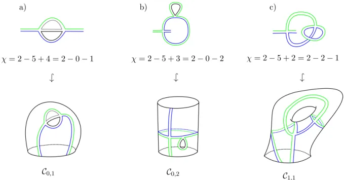
The upper row of Figure 1 shows three examples of ribbon graphs with n = 2 one-valent vertices andv= 2 four-valent vertices. In general, this construction lets the strands connect to n open lines and a certain number s loops. Due to the Kronecker-δs from pairs and vertices, every one of then+slines or loops carries a unique label. Every loop is labelled by a summation
χ= 2−5 + 4 = 2−0−1 χ= 2−5 + 3 = 2−0−2 χ= 2−5 + 2 = 2−2−1 C0,1 C0,2 C 1,1 , → ,→ ,→ a) b) c)
Figure 1. Three different ribbon graphs together with the associated Riemann surfacesCg,b. The external strands are coloured in green and blue. The topology ofCg,bis computed byχ=v−r+s= 2−2g−b.
index which is the remnant of the summation PN
j1,...,mv=1 in (4) after taking all Kronecker-δs into account. The open lines are labelled by the first matrix indices p1, .., pn of the product
Φp1q1· · ·Φpnqn in (4), and the integral (4) is zero unless there is a permutation π ∈ Sn with qi=π(pi) for all i= 1, ..., n. This permutationπ is uniquely1 determined by the ribbon graph,
simply by looking at the strand labels of the ribbon at every one-valent vertex.
Next, observe that due to the symmetry of the product Qvi=1 ΦjikiΦkiliΦlimiΦmiji
in (4) under cyclic permutation ji → ki → li → mi → ji of order 4 at every vertex and the v!
permutations of the vertices there are 4vv! pairings which give the same labelled ribbon graph. We can thus omit the factor 4v1v! and sum only over the different labelled ribbon graphs. This expresses the integral (4) as follows:
Proposition 3.1. Let p1, ..., pn be pairwise different and Gv,πp1,...,pn be the set of labelled con-nected ribbon graphs with v four-valent vertices and n one-valent vertices labelled (p1, π(p1)), . . . , (pn, π(pn)). Then for n even the integral (4) evaluates to
Nnhep1π(p1)...epnπ(pn)ic= ∞ X v=0 X Γ∈Gv,πp1,...,pn Nv−r+n+s(Γ)$(Γ), (5)
where r= 2v+n/2is the number of ribbons, s(Γ) the number of loops inΓ and the weight$(Γ) is derived from the following Feynman rules:
• label the s=s(Γ) loops by k1, ..., ks;
• associate a factor −λto a 4-valent ribbon-vertex;
• associate the factor E 1
p+Eq to a ribbon with strands labelled by p, q;
• multiply all factors and apply the summation operator N1s PN
k1,..,ks=1.
The exponent χ := v−r +n+s(Γ) of N in (5) has a topological interpretation. Let b be the number of cycles in π. We take b auxiliary faces, called boundary components, and
1
attach the one-valent vertices in cyclic order and according to the cycle they belong to to the circumference of the boundary components. The edge between two neighboured vertices on a boundary component closes an open line of Γ. In total this produces n additional loops. We thus get a simplicial 2-complex of v+n vertices, r +n edges and b+n+s faces, hence of Euler characteristic 2−2g = (v +n) −(r+n) + (b+n+s). This identifies the exponent χ= 2−2g−b=v−r+n+sof N as the Euler characteristic of a bordered Riemann surface
Cg,b(Γ). It is, up to homotopy, uniquely defined2 by the simplicial 2-complex encoded in Γ. The
lower row of Figure 1 sketches the bordered Riemann surfaces defined by the corresponding ribbon graphs of the first row.
To compare with the solution via Dyson-Schwinger equations we give an equivalent formu-lation of (5). A ribbon graph Γ ∈ Gv,πp1,...,pn contains full information about the cycle type of π ∈ Sn and about which of the p1, ..., pnlabel a chosen cycle of π. We rearrange these labels as
follows. Setp11 :=p1and then recursivelyp1k :=π1−k(p11) fork= 2, ..., n1ifπ−n1(p11) =p11. Next relabel any of the not yet assignedpk asp21 and continue to set p2k:=π1
−k(p1
2) fork= 2, ..., n2 if π−n2(p1
2) =p22. Proceed until the relabelling is complete. We denote byGv|p1
1...p1n1|...|pb1...pbnb|the set of relabelled ribbon graphs inGv,πp1,...,pn; both sets are in one-to-one correspondence. We further partition this set as Gv|
p1 1...p1n1|...|pb1...pbnb| = S∞ g=0G g,v |p1
1...p1n1|...|pb1...pbnb| into subsets of graphs of the same genusg. For fixedv, this union is actually finite. With these preparations we can represent the series coefficients of the genus expansion G|p1
1...p1n1|...|pb1...pbnb| = P∞ g=0N−2gG (g) |p1 1...p1n1|...|pb1...pbnb| of (3) for pairwise different pji ∈ {1, ..., N} as
G(|pg1) 1...p1n1|...|pb1...pbnb|= ∞ X v=0 X Γ∈Gg,v |p11...p1n1|...|pb1...pbnb| $(Γ). (6)
Remark 3.2. One can define similar structures for the logarithm of the partition function itself, logZ = logR
HN0 dµE,0(Φ)e
−λN
4 Tr(Φ4). LetGg,v
∅ be the set of connected vacuum ribbon graphs of
genusg made ofv four-valent vertices and no one-valent vertices. Then the analogue of (5) is
logZ = ∞ X g=0 ∞ X v=0 X Γ0∈Gg,v∅ N2−g$(Γ0) |Aut(Γ0)| , (7)
where$(Γ0) is given by the same Feynman rules as in Proposition3.1and|Aut(Γ0)|is the order of the automorphism group3 of the vacuum ribbon graph Γ0.
Later in Definition4.1we will introduce the free energy. We can perturbatively establish
F(g)=−δg,0 2N2 N X k,l=1 log(Ek+El) + ∞ X v=1 X Γ0∈Gg,v∅ $(Γ0) |Aut(Γ0)| . (8) 3.2 Examples
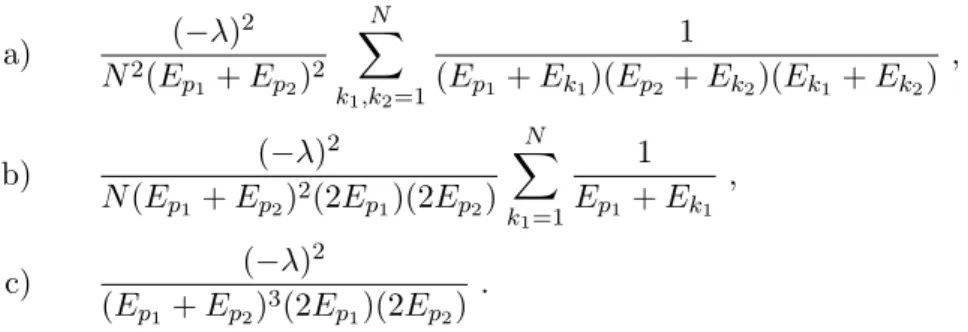
Example 3.3. For the ribbon graphs of Figure 1, we label the green open line by p1 and
the blue open line by p2. Consequently, the graphs become elements of G0|p,2
1p2|,G
0,2
|p1|p2|,G
1,2
|p1p2| 2The dual graph of a connected ribbon graph Γ associated toC
g,b is a quadrangulation (a map) ofCg,b. Our
definition of the correlation functions by disjoint cycles is equivalent to the definition used in [1] for fully simple maps. Fully simple maps are a subset of ordinary maps which are usually studied in matrix models (see [1] for more details).
3
respectively. The weights$(Γ) associated to these ribbon graphs are a) (−λ) 2 N2(E p1 +Ep2)2 N X k1,k2=1 1 (Ep1 +Ek1)(Ep2 +Ek2)(Ek1 +Ek2) , b) (−λ) 2 N(Ep1 +Ep2)2(2Ep1)(2Ep2) N X k1=1 1 Ep1 +Ek1 , c) (−λ) 2 (Ep1 +Ep2)3(2Ep1)(2Ep2) .
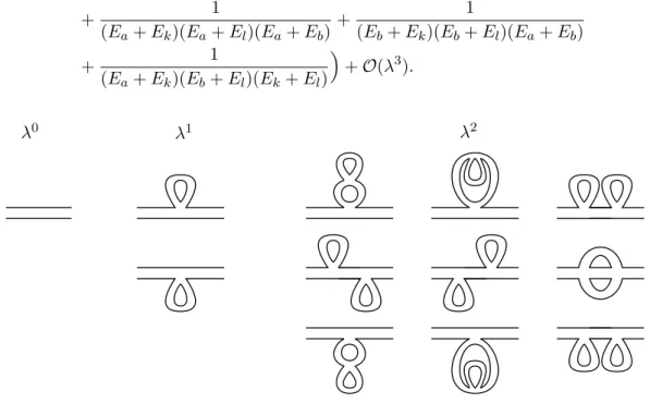
Example 3.4. The free energy F(0) of genus g = 0 consists of the empty ribbon graph with
weight given by the first term in (8) and 4 ribbon graphs up to order λ2 (see Figure2). Taking weights and order of the automorphism groups into account, we have perturbatively
F(0)= −1 2N2 N X k,l=1 log(Ek+El) + (−λ) 2N3 N X k,l,m=1 1 (Ek+El)(Ek+Em) +(−λ) 2 2N4 N X j,k,l,m=1 1 (Ej+Em)(Ej +Ek)2 1 Ej+El + 1 Ek+El +(−λ) 2 8N4 N X j,k,l,m=1 1
(Ej+Ek)(Ek+El)(El+Em)(Em+Ej)
+O(λ3).
λ1 λ2
λ0
Figure 2. The graph at orderλ0 is added as the empty ribbon graph. All these graphs contribute to
the free energy of genus 0 up to orderλ2. These graphs are elements ofG0∅,v. The melon graph ΓM has |Aut(ΓM)|= 8 and the other four graphs|Aut(Γ)|= 2.
Example 3.5. The first example with one boundary component is the 2-point function to which
12 ribbon graphs contribute up to orderλ2 (see Figure3). Taking the weights into account, we have perturbatively G(0)|ab|= 1 Ea+Eb + (−λ) (Ea+Eb)2 1 N N X k=1 1 Ea+Ek + 1 Eb+Ek + (−λ) 2 (Ea+Eb)2 1 N2 N X k,l=1 1 (Ea+Ek)2(Ea+El) + 2 (Ea+Ek)(Eb+El)(Ea+Eb) + 1 (Eb+Ek)2(Eb+El) + 1 (Ea+Ek)2(Ek+El) + 1 (Eb+Ek)2(En+El)
+ 1 (Ea+Ek)(Ea+El)(Ea+Eb) + 1 (Eb+Ek)(Eb+El)(Ea+Eb) + 1 (Ea+Ek)(Eb+El)(Ek+El) +O(λ3). λ0 λ1 λ2
Figure 3. All graphs contributing to the 2-point functionG(0)|ab|up to orderλ2, where the upper strand
is labelled byaand the lower bybfor each graph. Topologically, some graphs are the same but different elements ofG0|ab,v| due to different labellings.
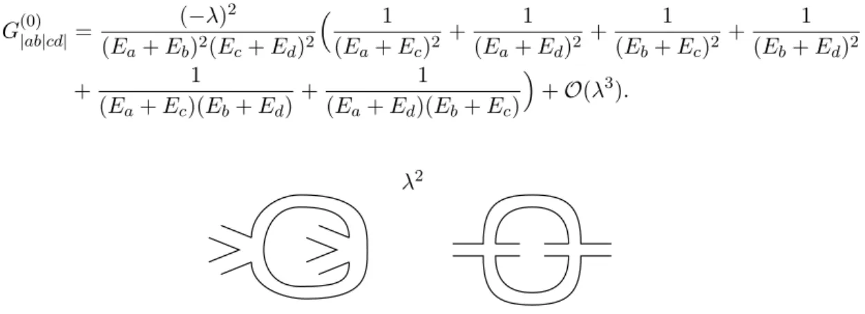
Example 3.6. The second example will be the 4-point function to which 11 graphs contribute
up to order λ2 (see Figure4). Taking the weights into account, we have perturbatively
G(0)|abcd|= (−λ)
(Ea+Eb)(Eb+Ec)(Ec+Ed)(Ed+Ea)
+ (−λ)
2
(Ea+Eb)(Eb+Ec)(Ec+Ed)(Ed+Ea)
× 1 N N X k=1 1 (Ea+Ek)(Ea+Eb) + 1 (Ea+Ek)(Ea+Ed) + 1 (Eb+Ek)(Eb+Ec) + 1 (Eb+Ek)(Eb+Ea) + 1 (Ec+Ek)(Ec+Ed) + 1 (Ec+Ek)(Ec+Eb) + 1 (Ed+Ek)(Ed+Ea) + 1 (Ed+Ek)(Ed+Ec) + 1 (Eb+Ek)(Ed+Ek) + 1 (Ea+Ek)(Ec+Ek) +O(λ3). λ1 λ2
Figure 4. All graphs contributing to the 4-point function G(0)|abcd| up to orderλ2, where the first two
graphs of orderλ2contribute with 4 different labellings and the last graph with 2 different labellings. In
total this gives 10 different labelled ribbon graphs which contribute at orderλ2. These 11 labelled graphs are elements ofG0|abcd,v |.
Example 3.7. The third example will be the (2+2)-point function to which 2 unlabelled ribbon graphs contribute up to orderλ2 (see Figure5). Taking the the weights into account, these split into 6 labelled ribbon graphs, leading to a perturbative expansion
G(0)|ab|cd|= (−λ) 2 (Ea+Eb)2(Ec+Ed)2 1 (Ea+Ec)2 + 1 (Ea+Ed)2 + 1 (Eb+Ec)2 + 1 (Eb+Ed)2 + 1 (Ea+Ec)(Eb+Ed) + 1 (Ea+Ed)(Eb+Ec) +O(λ3). λ2
Figure 5. All graphs contributing to the (2+2)-point functionG(0)|ab|cd| up to orderλ2, where the left
graph contributes with 4 different versions for the labelling and the right graph with 2 different versions for the labelling of the strands. This means thatG0|ab,2|cd|consists of 6 elements.
It is clear from the Feynman rules of Proposition 3.1 that at each order the correlation functions are rational functions of Epj
i and Eki. Consequently the limit to coinciding indices pji →pji00 is well-defined at any order in λ.
For any ni > 2, recursive algebraic relations between correlation functions are known; we
refer to [20] for the general formula. In case of (g, b) = (0,1), the algebraic relation for the n1-point function of genus zero is
G(0)|p 1p2...pn1|=−λ n1−2 2 X k=1 G(0)|p 2k+2...pn1p1|G (0) |p2...p2k+1|−G (0) |p2k+1...pn1|G (0) |p1...p2k| (Ep2k+1−Ep1)(Ep2 −Epn1) .
The explicit combinatorial structure of this recursive equation was understood in [12] in form of two nested combinatorial problems each governed by Catalan numbers.
Example 3.8. The 4-point function is algebraically expressed in terms of the 2-point function
by G(0)|abcd|=−λG (0) |ad|G (0) |bc|−G (0) |ab|G (0) |cd| (Ec−Ea)(Eb−Ed) .
The reader can check that this equation holds at the first two orders by inserting Example 3.5 into the rhs to recover Example 3.6.
4
Auxiliary Functions of Topological Significance
4.1 Creation Operator The derivative ˆ Tq:=−N ∂ ∂Eq
with respect to the parameters of the free theory, which we call boundary creation operator, plays a central rˆole in [6]. It is used to define the auxiliary functions
Tq 1,q2,...,qmkp11...p1n1|p21...p2n2|...|pb1...pbnb|:= ˆTq1. . . ˆ TqmG|p1 1...p1n1|p21...pn22|...|pb1...pbnb| Ωq1,...,qm := ˆTq2. . .TˆqmΩq1+ δm,2 (Eq1−Eq2)2 , m≥2, (9) where Ωq:= 1 N N X k=1 G|qk|+ 1 N2G|q|q|.
To define these functions properly it is necessary that allqi, pji are pairwise different. As before we
introduce genus expansions Tq
1,q2,...,qmkp11...p1n1|...|pb1...pbnb| = P∞ g=0N −2gT(g) q1,q2,...,qmkp11...pn11|...|pb1...pbnb| and Ωq1,...,qm = P∞ g=0N−2gΩ (g) q1,...,qm
Definition 4.1. The free energyFis defined to be a primitive of Ωqunder the creation operator,
i.e. Ω(qg)=: ˆTqF(g).
Main tool to evaluate applications of ˆTq is the equation of motion [26, Lemma 2] which can
be reformulated as 1 N ∂logZ(M) ∂Eq = N X k=1 ∂2logZ(M) ∂Mqk∂Mkq +∂logZ(M) ∂Mqk ∂logZ(M) ∂Mkq + 1 N N X k=1 G|qk|+ 1 N2G|q|q|. (10)
The following proposition gives the exact result for a single ˆTq-operation. In its proof the
assumption that the pji are pairwise different and different from q is essential. For application of another ˆTq0 on the result such an assumption does not hold. The calculation of several
ˆ
T-operations must be carefully repeated.
Proposition 4.2. For J =p11...p1n1|p21...p2n2|...|pb1...pbnb ≡ {J1, ..., Jb} and Ji = [pi1, ..., pini] with all pjl pairwise different and different from q one has
ˆ TqG(|J |g) = 1 N N X k=1 G|J |(g)qk|+G|J |(g−q1)|q|+ b X j=1 nj X l=1 G(g) |[q,pjl].lJj|J \Jj| + X g1+g2=g J1]J2=J G(g1) |J1|q|G (g2) |J2|q|,
where [p1, p2, ..., pi].l[q1, q2, ..., qj] := [q1, ..., ql, p1, ..., pi, ql+1, ..., qj] denotes the insertion of the first tuple after the lth position of the second tuple, l= 0, . . . , j.
Proof . As in [6] we introduce derivative operators DMD|J |J = D |J1| DMJ1 · · ·D |J b| DJ b with Dn DM[p1,...,pn] := (−iN)n∂n
∂Mp1p2...∂Mpn−1pn∂Mpnp1. This gives a representation G|J |=N
b−2 D|J | DMJ logZ(M) M=0 to which we apply ˆTq via (10): ˆ TqG|J | =Nb−2 N X k=1 D|J | DMJ −N2∂ 2logZ(M) ∂Mqk∂Mkq − N2∂logZ(M) ∂Mqk ∂logZ(M) ∂Mkq M=0 = 1 N N X k=1 G|J |qk|+ 1 N2G|J |q|q|+ b X j=1 nj X l=1 G|[q,pj l].lJj|J \Jj|+ X J1]J2=J G|J1|q|G|J2|q|.
The second line results from the first line by the following considerations. The first term Nb−2DMD|J |J
D2(logZ(M))
(a) For generick it produces N1G|J |qk|.
(b) For k=q it produces, besides N1G|J |qq| included in (a), also N12G|J |q|q| when interpreting
D2 DM[q,q] = D DM[q] D DM[q].
(c) Fork=pjl it produces, besides N1G|J |qpj l|
included in (a), alsoG|[q,pj
l].lJj|J \Jj|when taking Dnj DM[p j 1,...,p j nj] D2 DM[q,p j l] = Dnj+2 DM[p j 1,...,p j l,q,p j l,p j l+1,p j nj] into account.
The second term of the first line only contributes for k=q and for partitions of DMD|J |J into two
blocks J =J0] J00 which preserve the Jj individually. Indeed, any splitting of the Dn
DM[p1,...,pn]
applied to Z(M) gives zero when settingM = 0.
Inserting G... = P∞g=0N−2gG(...g) in the second line and extracting the coefficient of N−2g
gives the assertion.
Example 4.3. The action of the creation operator on the 2-point function reads
ˆ TqG(|pg1)p2|= 1 N N X k=1 G(|pg) 1p2|qk|+G (g−1) |p1p2|q|q|+G (g) |p1qp1p2|+G (g) |p1p2qp2|.
Example 4.4. The action of the creation operator on the (1 + 1)-point function reads
ˆ TqG(|pg1)|p2|= 1 N N X k=1 G(|pg1)|p2|qk|+G (g−1) |p1|p2|q|q|+G (g) |p1qp1|p2|+G (g) |p1|p2qp2|+ X g1+g2=g G(g1) |p1|q|G (g2) |p2|q|.
We also give a perturbative proof of Proposition 4.2. The creation operator ˆTq takes the
derivative with respect to Eq of a rational function arising from the Feynman rules in
Propo-sition 3.1. Since all external indices pji are by assumption different from q, the derivative hits only the sums of the internal strands (loops) if the summation index coincides with q. Being a derivative, it is the sum over all strands of all internal loops. Isolating every such target as
1 N N X k=1 1 Ek+Em f(Ek, Em, ...), (11)
wheref(Ek, Em, ...) is a rational function inEk, Em and further Ej, then the creation operator
generates ˆ Tq 1 N N X k=1 1 Ek+Em f(Ek, Em, ...) → 1 (Eq+Em)2 f(Eq, Em, ...).
Graphically, a ribbon with internal strand labelled by kis hit by the creation operator ˆTq. Its
ribbon is cut into two ribbons each with weight E 1
q+Em, where the previous loop labelkis now fixed to q. Depending on the type of the other index m and the topology of the graph, four classes of ribbon graphs can be produced by action of ˆTq:
1. The creation operator ˆTq acts on a ribbon in which both strands are internal strands, but
different from each other. This means that mabove is another summation index to which a summation operator N1 PNm=1 is assigned. The ribbon graph resulting from application of ˆTq thus receives an additional boundary component with 2 one-valent vertices with
one strand fixed to q and the other to m with a summation over m. All other boundary compenents of the previous ribbon graphs are untouched. The resulting graph contributes to N1 PNm=1G(|pg1)
m k → 1 N PN m=1 m q m q
2. The creation operator ˆTq acts on a ribbon, where both strands are internal strands and
the same, i.e. the indexmis also set tok. Here we consider the case that after cutting the ribbon, the ribbon graph is still connected. Cutting the selected ribbon then decreases the genus by 1; otherwise it is not possible that both strands have the same label. Acting with
ˆ
Tqon the other strand of the same ribbon leads to the same result, thus a total factor of 2.
The resulting graph has two additional boundary components each with 1 one-valent vertex with strands fixed to q. All other boundary compenents of the previous ribbon graphs are untouched. The resulting graph with its factor of 2 contributes to G(|g−1)
p1
1...p1n1|...|p
b
1...pbnb|q|q| . The factor of 2 accounts for the difference between labelled and unlabelled ribbon graphs. To see this consider G(|pg1−1)
1...p1n1|...|pb1...pbnb|q0|q00| withq
0
6
=q00 in which every topological ribbon graph occurs twice, namely first with labels q0, q00 on an ordered pair of open lines and second with labels q00, q0 on that pair. When setting q0 = q00 = q we get twice the same labelled ribbon graph.
k → 2× k q q q q
3. The creation operator ˆTq acts on a ribbon, where one strand is internal and the other
external, i.e. the indexmabove is somepjl. After cutting the ribbon, the previously internal strand becomes part of thejth boundary component. The resulting ribbon graph receives 2 additional one-valent vertices next to each other, with attached ribbons labelledpjlq and qpjl, at thejth boundary component. All otherb−1 boundary compenents are untouched. The resulting ribbon graph thus contributes to G(g)
|p11...p1n1|p j 1...p j l−1p j lqp j lp j l+1...p j nj|pb1...pbnb| . pjl k q pjl q pjl →
4. The creation operator ˆTq acts on a ribbon where both strands are internal strands of
the ribbon. Acting with ˆTq on the other strand also labelled k gives the same splitting,
thus a total factor of 2. Each of the two resulting connected ribbon graphs receives an additional boundary component with a single one-valent vertex whose ribbon is labelled qq. All previous boundaries with labelsJ as well as the total genusg are untouched, but split into each of the ribbon graphs. This splitting accounts for the additional factor of 2 because for given assignment J0,J00 the decompositions J0] J00 =J and J00] J0 =J are considered as different. The resulting ribbon graph thus contributes to G(g1)
|J1|q|G
(g2)
|J2|q|
with sum over g1+g2=g and over splittingsJ1] J2 =J. k → 2× k q q q q
Notice that for the vacuum ribbon graphs of the free energyF(g) only the two cases1 and2 contribute. Case 3 contributes only if a ribbon graph has an external strand, which is not the case for a vacuum ribbon graph, and case 4 does not contribute because any vacuum ribbon graph is a 1PI (one particle irreducible) due to four-valent vertices, i.e. after cutting a ribbon the graph stays connected.
Example 4.5. Take Example4.3 for g = 0 with its ribbon graph expansion. The first orders
of the expansion of the 2-point function are given in Example 3.5 with ribbon graphs drawn in Figure 3. The perturbative action of the creation operator described above generates the corresponding contributions of the 4-point function and the (2 + 2)-point function, which can be taken from the Examples 3.6 and 3.7, where the graphs are drawn in Figure 4 and 5. It is left to the reader to check the explicit formulae.
Example 4.6. The action of the creation operator on the free energy of genusg= 0 is
ˆ TqF(0)= 1 N N X k=1 G(0)|qk|.
Take the perturbative expansion of the free energy from Example3.4with ribbon graphs drawn in Figure2. The symmetry factor of the automorphism group of each ribbon graph ensures that the ribbon graphs generated by the creation operator have correct factors in agreement with Example3.5. Consequently, this gives a way to compute the order of the automorphism group. For instance, the contribution of the sunrise graph to N1 PNk=1G(0)|qk| is generated in 8 different ways by acting with the creation operator at the melon graph ΓM of F(0), which hence has |Aut(ΓM)|= 8.
We conclude that the action of the creation operator can be represented in two different but equivalent ways, first directly on the correlation functions by using manipulations of the partition function and second perturbatively by using the action on the weighted graphs.
4.2 Representation of Ω(g) in Terms of Correlation Functions
We have shown in [6] that the Ω(qg1),...,qm defined in (9) extend to meromorphic differential forms ωg,m on ˆCm for which we provided strong evidence that they obey blobbed topological recursion
[2]. If true theωg,nare relatively easy to obtain via evaluation of residues. The translation back
to Ω(qg1),...,qm is simple. In this section we give another representation of the Ω (g)
q1,...,qm as special polynomials in the correlation functions G(...g0). The purpose is twofold. First, comparison of a perturbative expansion of the G(...g0) with a Taylor expansion of the exact formulae provides an
important consistency check. Second, we understand our observation as a message for quantum field theory in general: Also in realistic QFT it might be worthwhile to investigate whether certain polynomials of correlation functions, which themselves are Feynman graph series, reveal a deeper structure than individual functions or graphs.
The definition already gives Ω(qg1) =
1 N PN k=1G (g) |q1k|+G (g−1)
|q1|q1|. The next two propositions
provide Ω(qg1),q2 and Ω
(g)
q1,q2,q3. It would be straightforward but increasingly lengthy to continue.
Proposition 4.7. Forq16=q2 one has
Ω(qg1),q2 = δg,0 (Eq1−Eq2)2 + X g1+g2=g G(g1) |q1q2|G (g2) |q1q2| + 1 N2 N X k,l=1 G(|qg) 1k|q2l|+ 1 N N X k=1 G(|qg) 1kq1q2|+G (g) |q2kq2q1|+G (g) |q1kq2k| + 1 N N X k=1 G(|qg−1) 1k|q2|q2|+G (g−1) |q2k|q1|q1| +G(|qg−1) 1q2q2|q2|+G (g−1) |q2q1q1|q1| + X g1+g2=g−1 G(g1) |q1|q2|G (g2) |q1|q2|+G (g−2) |q1|q1|q2|q2|. (12) Proof . Using Ωq1 = 1 N2 PN k=1 D 2 DM[q1,k] logZ(M) M=0 and (10) we have ˆ Tq2Ωq1 =− N X k,l=1 D2 DM[q1,k] ∂2logZ(M) ∂Mq2l∂Mlq2 +∂logZ(M) ∂Mq2l ∂logZ(M) ∂Mlq2 M=0 (13) = 1 N2 N X k,l=1 G|q1k|q2l|+ 1 N N X k=1 G|q1kq1q2|+G|q2kq2q1|+G|q1kq2k| +G|q1q2|G|q1q2| + 1 N3 N X k=1 G|q1k|q2|q2|+G|q2k|q1|q1| + 1 N2 G|q1q2q2|q2|+G|q2q1q1|q1| + 1 N2G|q1|q2|G|q1|q2|+ 1 N4G|q1|q1|q2|q2|.
The last two lines result from the first line of (13) as follows. The first term N12 D 2
DM[q1,k]
D2(logZ(M))
DM[q2,l]
contributes in nine different ways:
(a) For generick, l it produces N12G|q1k|q2l| summed overk, l.
(b) For l =q1 it produces, besides N12G|q1k|q2q1| included in (a), also
1 NG|q1kq1q2| when inter-preting D2 DM[q1,k] D2 DM[q2,q1] = D4 DM[q1,k,q1,q2].
(c) For k = q2 it produces, besides N12G|q1q2|q2l| included in (a), also
1 NG|q2lq2q1| when inter-preting D2 DM[q1,q2] D2 DM[q2,l] = D4 DM[q2,l,q2,q1]. We replace l7→k. (d) Forl=kit produces, besidesN12G|q1k|q2k|included in (a), also
1 NG|q1kq2k|when interpreting D2 DM[q1,k] D2 DM[q2,k] = D4 DM[q1,k,q2,k].
(e) Forl=q2 it produces, besides N12G|q1k|q2q2|included in (a), also
1 N3G|q1k|q2|q2|when inter-preting D2 DM[q1,k] D2 DM[q2,q2] = D2 DM[q1,k] D1 DM[q2] D1 DM[q2].
(f) Fork=q1 it produces, besides N12G|q1q1|q2l|included in (a), also
1 N3G|q2l|q1|q1|when inter-preting D2 DM[q1,q1] D2 DM[q2,l] = D2 DM[q2,l] D1 DM[q1] D1 DM[q1]. We replace l7→k.
(g) Fork=l=q2it produces, besides the three casesN12G|q1q2|q2q2|included in (a),
1
NG|q2q2q2q1|
included in (c) and N13G|q1q2|q2|q2| included in (e), also
1 N2G|q1q2q2|q2| when interpreting D2 DM[q1,q2] D2 DM[q2,q2] = D3 DM[q1,q2,q2] D1 DM[q2].
(h) Fork=l=q1it produces, besides the three casesN12G|q1q1|q2q1|included in (a),
1
NG|q1q1q1q2|
included in (b) and N13G|q2q1|q1|q1| included in (f), also
1 N2G|q2q1q1|q1| when interpreting D2 DM[q1,q1] D2 DM[q2,q1] = D3 DM[q2,q1,q1] D1 DM[q1].
(i) For k = q1 and l = q2 it produces, besides the three cases N12G|q1q1|q2q2| included in (a),
1
N3G|q1q1|q2|q2| included in (e) and
1 N3G|q1|q1|q2q2| included in (f), also 1 N4G|q1|q1|q2|q2| when interpreting DMD[q21,q1] D2 DM[q2,q2] = D1 DM[q1] D1 DM[q1] D1 DM[q2] D1 DM[q2].
The first term − 1
N2 D2 DM[q1,k] ∂logZ(M) ∂Mq2l ∂logZ(M)
∂Mlq2 contributes in two different ways
(a) Either k = q2 and l = q1 and derivatives distributed into N12
D2logZ(M)
DM[q1,q2]
D2logZ(M)
DM[q1,q2] = G|q1q2|G|q1q2|,
(b) or k = q1 and l = q2 and derivatives distributed into N12
D2logZ(M) DM[q1]DM[q2] D2logZ(M) DM[q1]DM[q2] = 1 N2G|q1|q2|G|q1|q2|.
Including the special term (E 1
q1−Eq2)2 and extracting the coefficient of N
−2g gives the assertion.
Proposition 4.8. For pairwise different q1, q2, q3 one has
Ω(qg1),q2,q3 = 1 N3 N X j,k,l=1 G(|qg) 1j|q2k|q3l|+ 1 N2 N X k,l=1 G(|qg) 1kq2k|q3l|+G (g) |q2kq3k|q1l|+G (g) |q3kq1k|q2l| +G(|qg) 1kq1q2|q3l|+G (g) |q1kq1q3|q2l|+G (g) |q2kq2q3|q1l|+G (g) |q2kq2q1|q3l|+G (g) |q3kq3q1|q2l|+G (g) |q3kq3q2|q1l| + 1 N N X k=1 G(|qg) 1kq2kq3k|+G (g) |q1kq3kq2k| +G(|qg) 1kq1q2q1q3|+G (g) |q1kq1q3q1q2|+G (g) |q2kq2q3q2q1|+G (g) |q2kq2q1q2q3|+G (g) |q3kq3q1q3q2|+G (g) |q3kq3q2q3q1| +G(|qg) 1kq1q2q3q2|+G (g) |q1kq1q3q2q3|+G (g) |q2kq2q3q1q3|+G (g) |q2kq2q1q3q1|+G (g) |q3kq3q1q2q1|+G (g) |q3kq3q2q1q2| +G(|kqg) 1kq2q3q2|+G (g) |kq1kq3q2q3|+G (g) |kq2kq3q1q3|+G (g) |kq2kq1q3q1|+G (g) |kq3kq1q2q1|+G (g) |kq3kq2q1q2| + 2 X g1+g2=g 1 N N X k=1 G(g1) |q1q2|G (g2) |q3k|q1q2|+G (g1) |q1q2|G (g2) |q1q2q1q3|+G (g1) |q1q2|G (g2) |q2q1q2q3| +G(g1) |q2q3|G (g2) |q1k|q2q3|+G (g1) |q2q3|G (g2) |q2q3q2q1|+G (g1) |q2q3|G (g2) |q3q2q3q1| +G(g1) |q3q1|G (g2) |q2k|q3q1|+G (g1) |q3q1|G (g2) |q3q1q3q2|+G (g1) |q3q1|G (g2) |q1q3q1q2| + 1 N2 N X k,l=1 G(|qg−1) 1k|q2l|q3|q3|+G (g−1) |q2k|q3l|q1|q1|+G (g−1) |q3k|q1l|q2|q2| + 1 N N X l=1 G(|qg−1) 1q1q2|q3l|q1|+G (g−1) |q1q1q3|q2l|q1|+G (g−1) |q2q2q3|q1l|q2|+G (g−1) |q2q2q1|q3l|q2| +G(|qg−1) 3q3q1|q2l|q3|+G (g−1) |q3q3q2|q1l|q3|
+G(|qg−1) 1q1q2q3q2|q1|+G (g−1) |q1q1q3q2q3|q1|+G (g−1) |q2q2q3q1q3|q2|+G (g−1) |q2q2q1q3q1|q2| +G(|qg−1) 3q3q1q2q1|q3|+G (g−1) |q3q3q2q1q2|q3|+G (g−1) |q1q1q2q1q3|q1|+G (g−1) |q1q1q3q1q2|q1| +G(|qg−1) 2q2q3q2q1|q2|+G (g−1) |q2q2q1q2q3|q2|+G (g−1) |q3q3q1q3q2|q3|+G (g−1) |q3q3q2q3q1|q3| +G(|qg−1) 1q1q2|q1q1q3|+G (g−1) |q2q2q3|q2q2q1|+G (g−1) |q3q3q1|q3q3q2| + 1 N N X k=1 G(|qg−1) 1kq2k|q3|q3|+G (g−1) |q2kq3k|q1|q1|+G (g−1) |q3kq1k|q2|q2|+G (g−1) |q1kq1q2|q3|q3|+G (g−1) |q1kq1q3|q2|q2| +G(|qg−1) 2kq2q3|q1|q1|+G (g−1) |q2kq2q1|q3|q3|+G (g−1) |q3kq3q1|q2|q2|+G (g−1) |q3kq3q2|q1|q1| + 2 X g1+g2=g−1 G(g1) |q1q2|G (g2) |q1q2|q3|q3|+G (g1) |q2q3|G (g2) |q2q3|q1|q1|+G (g1) |q3q1|G (g2) |q3q1|q2|q2| + 4 X g1+g2=g−1 1 N N X k=1 G(g1) |q1|q2|G (g2) |q3k|q1|q2|+G (g1) |q2|q3|G (g2) |q1k|q2|q3|+G (g1) |q3|q1|G (g2) |q2k|q3|q1| + 4 X g1+g2=g−1 G(g1) |q1|q2|G (g2) |q2|q1q1q3|+G (g1) |q1|q2|G (g2) |q1|q2q2q3|+G (g1) |q2|q3|G (g2) |q3|q2q2q1| +G(g1) |q2|q3|G (g2) |q2|q3q3q1|+G (g1) |q3|q1|G (g2) |q1|q3q3q2|+G (g1) |q3|q1|G (g2) |q3|q1q1q2| + 8 X g1+g2+g3=g−1 G(g1) |q1|q2|G (g2) |q2|q3|G (g3) |q3|q1| +G(|qg−2) 1q1q2|q3|q3|q1|+G (g−2) |q1q1q3|q2|q2|q1|+G (g−2) |q2q2q3|q1|q1|q2|+G (g−2) |q2q2q1|q3|q3|q2|+G (g−2) |q3q3q1|q2|q2|q3| +G(|qg−2) 3q3q2|q1|q1|q3|+ 1 N N X k=1 G(|qg−2) 1k|q2|q2|q3|q3|+G (g−2) |q2k|q3|q3|q1|q1|+G (g−2) |q3k|q1|q1|q2|q2| + 4 X g1+g2=g−2 G(g1) |q1|q2|G (g2) |q1|q2|q3|q3|+G (g1) |q2|q3|G (g2) |q2|q3|q1|q1|+G (g1) |q3|q1|G (g2) |q3|q1|q2|q2| +G(|qg−3) 1|q1|q2|q2|q3|q3|.
Proof . Applications of ˆTq3 to the first line of (13) gives with (10)
ˆ Tq3Tˆq2Ωq1 =N 2 N X j,k,l=1 D2 DM[q1,k] n ∂2 ∂Mq2l∂Mlq2 ∂2logZ(M) ∂Mq3j∂Mjq3 +∂logZ(M) ∂Mq3j ∂logZ(M) ∂Mjq3 + ∂ ∂Mq2l ∂2logZ(M) ∂Mq3j∂Mjq3 +∂logZ(M) ∂Mq3j ∂logZ(M) ∂Mjq3 ∂logZ(M) ∂Mlq2 + ∂ ∂Mlq2 ∂2logZ(M) ∂Mq3j∂Mjq3 +∂logZ(M) ∂Mq3j ∂logZ(M) ∂Mjq3 ∂logZ(M) ∂Mq2l o M=0 .
A similar discussion as before gives the assertion.
Using the previous Examples3.5,3.6and 3.7, it is easy to write Ω(0)q1 and Ω
(0)
q1,q2 up to order
λ2 and Ω(0)q1,q2,q3 up to orderλ
1.
5
Results Connected with Blobbed Topological Recursion
In the next subsection we briefly recall the main construction of [6] howexplicit and exact results for Ω(bg)
1,...,bn are obtained. Afterwards, the first few examples are expanded in λ and shown to reproduce the perturbative results.
5.1 Summary of Previous Work
Our main tool is the usage of Dyson-Schwinger equations. They are first derived for the corre-lation functions G(...g) introduced before, then complexified to functionsG(g) of several complex variables which satisfy G(g)(Ep1
1, ..., Ep1n1|...|Epb1, ..., Epbnb) = G (g) |p1 1...p1n1|...|p b 1,...,pbnb| . After complex-ification one can admit multiplicities of the Ek, i.e. we assume that (e1, ..., ed) are the
pair-wise different values in (E1, ..., EN) which arise with multiplicities (r1, ..., rd), respectively, with
r1+...+rd = N. It is also straightforward to take a limit where the ek continuously fill an
interval with a certain spectral measure. As mentioned before, there is a closed non-linear equa-tion [18,19] for the planar 2-point function alone and an infinite hierarchy of affine equations for all other functions. A continuum variant of the non-linear equation was solved in [25] for the 2-dimensional Moyal case and later in [16] in full generality. It suggested an ansatz in which an implicitly defined function R: ˆC→Cˆ, where ˆC=C∪ {∞}, is crucial:
Theorem 5.1 ([26]). Let (E1, ..., EN) be partitioned into pairwise different e1, ..., ed>0 which arise with multiplicities (r1, ..., rd), respectively. Assume that the complexification Ωˆ(0)(Eq) =
Ω(0)q can be expressed as ˆ Ω(0)(R(z)) =: Ω(0)1 (z) =−R(−z) +R(z) λ − 1 N d X k=1 rk R(εn)−R(z)
for some meromorphic function R of degee d+ 1with R(εk) =ek and R(∞) =∞. Then R is, for generic values of (ek), uniquely determined by the non-linear Dyson-Schwinger equation to
R(z) :=z− λ N d X k=1 %k εk+z , %k= rk R0(ε k) . (14)
Choosing limλ→0εk =ek, then any(ek) is generic forλin an open (real or complex) neighbour-hood of 0.
The implicitly defined function R provides a ramified covering R : ˆC → Cˆ of Riemann
spheres, see Figure 6. The important observation is that R pulls ˆΩ(0)(ζ) back to a rational function Ω(0)1 (z). This rationality on the (right)z-plane of Fig.6extends to all other correlation functions. In contrast, when expressing these functions in terms of the original variables (ek)
we need to invertR which in closed form is not possible beside d= 1.
e1 e2 ... ed R−1 U V ε1 ε2 ... εd Im(ζ) Re(ζ) Im(z) Re(z) R
Figure 6. Illustration of the ramified covering map R : ˆC→Cˆ satisfyingR(εk) =ek. The mapR is biholomorphic between the neighbourhoodsV andU.
It was understood in [6] that, although all other complexified functions G(g) satisfy affine Dyson-Schwinger equations (see [20]), an explicit solution must first be achieved for the auxiliary functions Ωm(g)(z1, ..., zm) with Ωm(g)(εq1, ..., εqm) = Ω
(g)
q1,...,qm. We refer to [6] for details about the solution strategy for Ω(mg)(z1, ..., zm). Here we only quote the remarkably simple result:
Proposition 5.2 ([6]). Let R(z) be as in Theorem 5.1 and βi for i ∈ {1, ...,2d} be the 2d solutions of R0(z) = 0. We have the solutions
Ω(0)2 (u, z) = 1 R0(u)R0(z) 1 (u−z)2 + 1 (u+z)2 , (15) Ω(0)3 (u, v, z) = 1 R0(u)R0(v)R0(z) ∂3 ∂u∂v∂z h λ 1 v+u + 1 v−u R0(u)R0(−u)(z+u)+ λ u+1v +u−1v R0(v)R0(−v)(z+v) + 2d X i=1 λ v+1β i + 1 v−βi 1 u+βi + 1 u−βi R0(−β i)R00(βi)(z−βi) i . (16)
The function Ω(0)3 (u, v, z) is completely symmetric in its arguments.
In [6] also the solutions of Ω(mg) with (g, m) = (0,4),(1,1) are derived. All these results
underpin the conjecture that meromorphic formsωg,mdefined byω0,1(z) =−R(−z)R0(z)dzand for 2g+m ≥0 by ωg,m(z1, ..., zm) = Ωm(g)(z1, ..., zm)Qmj=1R0(zj)dzj follow blobbed topological
recursion for the spectral curve
(x: Σ→Σ0, ω0,1(z), B(u, z)) = R: ˆC→Cˆ,−R(−z)dR(z), du dz (u−z)2 .
This means that the poles of ωg,m at the ramification points βi ofR are given by the universal
formula of topological recursion. These are enriched by further contributions, called blobs, which for the Quartic Kontsevich Model have poles at zi = 0 andzi+zj = 0. Their general structure
is not yet understood in our case. We refer to [14,13] for topological recursion in general and to [2] for blobbed topological recursion.
5.2 Comparison Between Exact Results and Weighted Ribbon Graphs
In this subsection we compare the exact solutions of Theorem5.1 and Proposition5.2 with the perturbative expansion via weighted ribbon graphs. First, we need the expansion of εa and
R0(εa) which is easily obtained by iterative insertion into the definition ofR(z). The first orders
yield: εq =eq+ λ N d X n=1 rn eq+en − λ2 N2 d X n,k=1 rnrk 1 (eq+en)(ek+en)2 + 1 (eq+en)2(eq+ek) + 1 (eq+en)2(en+ek) +O(λ3), R0(εq) = 1 + λ N d X n=1 rn (eq+en)2 − λ2 N2 d X n,k=1 rnrk 1 (eq+en)2(ek+en)2 + 2 (eq+en)3(eq+ek) + 2 (eq+en)3(en+ek) +O(λ3). Also necessary for (g, n) = (0,3) and higher topologies are the zeroesβi ofR0 (so-called
ramifi-cations points). Theλ-expansion yields
βi =−ei+ i r λri N − λ N d X n=1 rn ei+en +O λ32, βi+d= ¯βi i∈ {1, ..., d}. (17)
The expansions of εq and βi are easily implemented into a computer algebra system. Deriving
perturbative results for the Ω(ng)is then straightforward. We demonstrate this with the following
examples:
Example 5.3. From the expansion of the exact result, we obtain using Theorem5.1
Ω(0)1 (εq) = εq−eq λ + 1 N d X n=1 rn 1 R0(ε n)(εn−εq)− 1 en−eq = 1 N d X n=1 rn en+eq − λ N2 d X n,k=1 rnrk 1 (eq+en)(ek+en)2 + 1 (eq+en)2(eq+ek) + 1 (eq+en)2(en+ek) + 1 (en+ek)2(en−eq) + 1 en+ek − 1 eq+ek (en−eq)2 +O(λ2) = 1 N d X n=1 rn en+eq − λ N2 d X n,k=1 rnrk (eq+en)2(eq+ek) + rnrk (eq+en)2(en+ek) +O(λ2).
This result is in full compliance with the graph expansion of Example 3.5 inserted into Ω(0)q =
1
N PN
k=1G (0)
|qk|. The agreement is immediate forrn= 1; otherwise one collects rk identical terms
where Ek1 = ... = Ekrk = ek. The expansion of the exact result is represented in a different
partial fraction decomposition than the graph expansion. The reader may check also the next order.
Example 5.4. We obtain from Proposition 5.2
Ω(0)2 (εq, εr)− 1 (eq−er)2 = 1 R0(ε q)R0(εr) 1 (εq−εr)2 + 1 (εq+εr)2 − 1 (eq−er)2 = 1 (eq+er)2 − λ N d X n=1 rn 2 1 en+eq − 1 en+er (eq−er)3 + 1 (eq+en)2 + 1 (er+en)2 (eq−er)2 + 2 1 en+eq + 1 en+er (eq+er)3 + 1 (eq+en)2 + 1 (er+en)2 (eq+er)2 +O(λ2), which is in full compliance with the graph expansion of Examples3.5and3.6inserted into Propo-sition 4.7 (but in a different partial fraction decomposition). The reader may check the next order, where additionally the graphs of the (2 + 2)-point function from Example 3.7contribute.
Example 5.5. We obtain from Proposition 5.2
Ω(0)3 (εq, εr, εs) = 1 R0(ε q)R0(εr)R0(εs) h ∂ ∂u λ (ε 1 r+u)2 + 1 (εr−u)2 R0(u)R0(−u)(ε s+u)2 u=εq + ∂ ∂v λ (ε 1 q+v)2 + 1 (εq−v)2 R0(v)R0(−v)(ε s+v)2 v=εr − 2d X i=1 λ (ε 1 r+βi)2 + 1 (εr−βi)2 1 (εq+βi)2 + 1 (εq−βi)2 R0(−β i)R00(βi)(εs−βi)2 i =−λ·2 1 (er+eq)2 + 1 (er−eq)2 (es+eq)3 + 1 (er+eq)3 − 1 (er−eq)3 (es+eq)2 + 1 (eq+er)2 + 1 (eq−er)2 (es+er)3 + 1 (eq+er)3 − 1 (eq−er)3 (es+er)2 +O(λ2),
where the restrictions to u = εq and v =εr in the second line vanish. The only contributions
come from the i-summation. This result is in full compliance with the graph expansion in Examples 3.5 and 3.6 inserted into Proposition 4.8, but again in a different partial fraction decomposition. For the computation, we remark that the expansion
1 (εq+βq)2 =− N λrq +O√1 λ , 1 (εq+βq+d)2 =− N λrq +O√1 λ , 1 R00(βi) =−i 2 r λri N +O(λ), 1 R00(βi+d) = +i 2 r λri N +O(λ)
indicates a contribution of order √λ from the i-summation, which actually cancels due to the pairs (βi, βi+d) of complex conjugations ¯βi =βi+d. The reader may even check that the order
λ32 cancels as well.
5.3 Combinatorics
A common investigation in QFT concerns the growth of the number of Feynman graphs at a certain orderλv. In order to illustrate the enormous complexity of the individual contributions to
Ω(0)a and Ω(0)a,bat a given orderλv, we will calculate these numbers explicitly. To enter this regime
of enumerative geometry within the Quartic Kontsevich Model we have to set d= 1. We will now show how to expandG(0)|11|,G(0)|1111|andG(0)|11|11|(the 2-point, 4-point and (2+2)-point function for a single, (r1=N)-fold degenerate spectral valuee1 =e) in an exact and generic perturbative series in λ. The prefactors of (−λ)v for e = 12 then simply count the number of connected Feynman ribbon graphs contributing to the graph expansion at order v. As known from the Hermitian 1-matrix model [7], the duals of the ribbon graphs of the Quartic Kontsevich Model are rooted quadrangulations. However, due to a different definition of correlation functions, the correspondence to [7] is not one-to-one. To avoid complicated redefinitions, we follow another path.
To derive the exact power series in λ, return to Theorem 5.1 and solve the 2d implicitly defined equations for d= 1 explicitly. Forε1=ε, we solve them to
ε= 1 6(4e+ p 4e2+ 12λ), %= N 18λ(2e p 4e2+ 12λ−4e2+ 12λ). With the other preimage ˆε=−1
6(2e+ 2
√
4e2+ 12λ) one expresses4 the planar 2-point function
as
G(0)|11|≡G(0)(e, e)≡G(0)(R(ε), R(ε)) =:G(0)(ε, ε) =− 2ˆε (ε−ε)ˆ2 .
Admitting multiplicities rk in the definition (9) of Ω(0)q we find for d= 1 and r1 =N
Ω(0)q = 1 N d X k=1 rkG (0) |qk| −→ Ω (0) 1 =G (0) |11|=G (0)(ε, ε).
The same steps give for Ω(0)q1,q2 according to Proposition 4.7
Ω(0)q1,q2 = 1 (eq1 −eq2)2
+ (G(0)|q
1q2|)
2
4See [6] for details about the complexification procedure from correlation functions G(g)
... to meromorphic
functionsG(g) (. . .).
+ 1 N N X k=1 rk G(0)|q1kq1q2|+G(0)|q2kq2q1|+G(0)|q1kq2k| + 1 N2 N X k,l=1 rkrlG(0)|q1k|q2l| −→ lim eq1,eq2→e Ω(0)q1,q2 − 1 (eq1−eq1)2 =G(0)(ε, ε)2+ 3G(0)(ε, ε, ε, ε) +G(0)(ε, ε|ε, ε). A lengthy calculation shows
G(0)(ε, ε, ε, ε) = 8e+ 12 √ 4e2+ 12λ (2e+√4e2+ 12λ)3 −2(G (0)(ε, ε))2 , G(0)(ε, ε|ε, ε) = 6λ2 (e+√4e2+ 12λ/2)6 . (18)
Inserting theλ-expansion of these formulae above gives the number of ribbon graphs contributing to Ω(0)q and Ω(0)q1,q2 at a given order λv. In the following table we list these numbers up to order
λ5. Order Ω(0)q Ω(0)q1,q2 λ0 1 1 λ1 2 7 λ2 9 58 λ3 54 522 λ4 378 4941 λ5 2916 48411
Those numbers can be checked at low orders of λ counting the diagrams in Figs. 3, 4 and 5. Regarding Ω(0)q we encounter very special numbers. By duality these are the same as the numbers
mg=0(n) of planar (g= 0) quadrangulations withnfaces plus a (marked) boundary of length 2. We recall:
Lemma 5.6 ([13, Chap. 3.1.7]). The number mg=0(n) of rooted planar (g = 0) maps with n
quandrangles and a marked boundary of length 2 is given by
mg=0(n) = 2·3n·
(2n)!
n!(n+ 2)! = 2·3
n
·nC+ 2n .
The planar 2-point function for d= 1 itself generates these numbers together with weights 21e of the edges.
The result for the number of ribbon graphs of orderλn contributing to Ω(0)1,1 can be derived from the Taylor series of (18) whose first terms are
G(0)(ε, ε|ε, ε) = 6(−λ)2 (2e)6 + 108(−λ)3 (2e)8 + 1458(−λ)4 (2e)10 + 17820(−λ)5 (2e)12 +... G(0)(ε, ε, ε, ε) = (−λ) (2e)4 + 10(−λ)2 (2e)6 + 90(−λ)3 (2e)8 + 810(−λ)4 (2e)10 + 7425(−λ)5 (2e)10 +. . . .
Things become difficult for d= 2 when we introduce different weightse1, e2.
6
Critical Coupling Constants and Geometric Discussion
So far, we were able to show analytically the expected coincidence between the exact solutions from (blobbed) topological recursion of the Quartic Kontsevich Model and their perturbative expansion in the coupling constant λ. Many systems of statistical physics, quantum mechanics
and quantum field theory show critical phenomena and phase transitions when parameters take particular values. This section starts to explore such phenomena in the Quartic Kontsevich Model. More precisely, we exemplify transitions between different stratification types of the parameter space. This includes the appearance of higher-order ramifications in the crucial functionR identified in Theorem 5.1and transitions between different ramification profiles.
6.1 The Setup
The investigation of special cases of the Quartic Kontsevich Model already suggested certain values of λ at which a critical behaviour occurs. In [16] a scaling limit d, N → ∞ of (14) to a renormalised integral representation R(z) =z−λ(−z)D/2R0∞(t+1)D/%(t2)(dtt+1+z) was established,
with D∈ {0,2,4}the smallest dimension that gives a convergent integral. We recall:
• Letd= 1 with anN-fold degenerate eigenvalue [16]. This is the Hermitian 1-Matrix Model. We obtain R(ε) =ε−Nλ 2%ε =e where N% =R0(ε), with solution ε= (e+√4e2+ 12λ)/6 directly given by inversion of R. In standard conventions one should identify e= 12 which gives a critical valueλc=−1/12 below whichR−1 cannot be defined as map between real
functions.
• Let d → ∞ with spectral measure %(t) = 1, the two-dimensional Moyal plane. After renormalisation one obtains R(z) = z+λlog(1 +z) [25]. An integral representation for the planar 2-point function is only consistent forλ >− 1
log(4).
• Let d → ∞ with spectral measure %(t) = t, the four-dimensional Moyal plane: One finds R(z) = z2F1(αλ,1−αλ,2;−z) where αλ = arcsin(λπ)/π for |λ| ≤ 1π and αλ =
1
2+i arcosh(λπ)/πforλ≥ 1
π [17]. The singular value isλs=−1/π. Its mirrorλcrit= +1/π
is a special transition point where αλ is continuous but not differentiable. However,R(z)
itself crosses smoothly over λcrit.
Beyond these special cases, we mostly leave the realm of exact solutions. Existence of solutions in a real or complex neighbourhood of λ = 0 is guaranteed by the implicit function theorem which constructs 2dfunctions{εk(λ), %k(λ)}k=1,...,d from given dataek, rk= limλ→0(εk, %k). For
a first discussion we simplify the situation and take (εk, %k) as given data independently ofλ.
This ignores the condition rk ∈Z>0 (could be arbitrarily well approximated forN → ∞). We will mostly consider the the cased= 2.
6.2 Behaviour of the Ramification Points for d= 2
The cased= 2 describes a threefold covering and four ramification points. We scan the running of the ramification points β1,2 and their complex conjugate by a variation of the coupling con-stant. Because of −2Pdk=1εk =
P2d
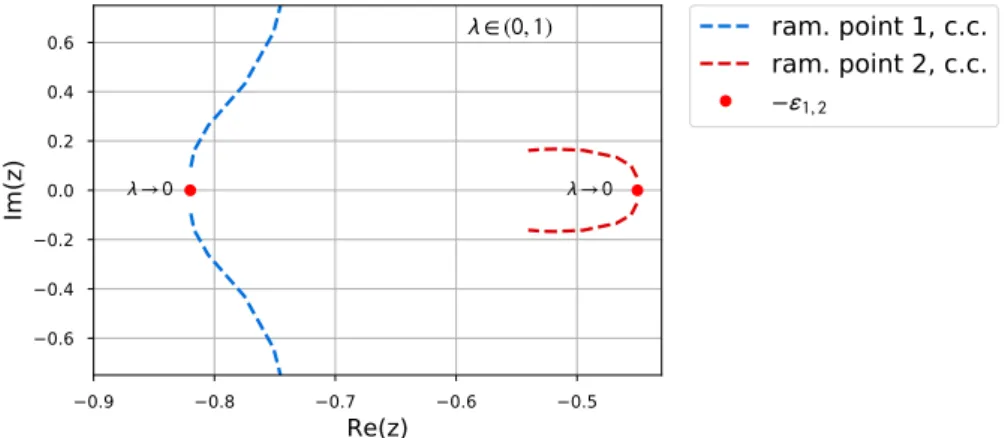
i=1βi (underpinning the perturbative expansions), which is a consequence of Vieta’s theorem, the variations of the βi sum up to zero. Figure7 shows the
typical situation. We rediscover the square root-like behaviour (17) for small λ.
Taking%1=%2, we reenter the regime of analytically solvable equations. Over and above, it shows a phenomenologically new behaviour:
Lemma 6.1. Given d = 2 parameters ε1 6= ε2 and suppose their multiplicities arrange to
%1 = %2 =: N %. Then two ramification points merge to a single higher ramification point β = β1 = β2 at the critical coupling constant λcrit = (ε1−ε2)
2
% . Its real part is a fixed point
R(Re(β)) = Re(β)) of R.
Proof . The value λcritis determined as follows: The four solutions of R0(z) = 0 read
β±,±= 1 2 −ε1−ε2± q (ε1+ε2)2−4 ε1ε2+λ%±p−λ%(ε1−ε2)2+λ2%2 .
0.9 0.8 0.7 0.6 0.5
Re(z)
0.6 0.4 0.2 0.0 0.2 0.4 0.6Im(z)
ram. point 1, c.c.
ram. point 2, c.c.
, ( , )Figure 7. For λ → 0, the ramification points propagate into −ε1 = −0.82 and −ε2 = −0.45 (these
values for εi are also chosen in Figs. 11 and 12, as well as %1 = 1, %2 = 3). In sum, the deformations
average to zero.
Then λ = 0 and λcrit = (ε1
−ε2)2
% are the solution where two roots merge. Let β1, β2 be the
solutions in the upper half plane. Then Im(β1) = Im(β2) > 0 for λ < λcrit and Re(β1) = Re(β2) =−ε1+ε2
2 =: −ε¯for λ > λcrit. For obvious reasons this value is a fixed point ofR, i.e. R(−ε) =¯ −ε. This order-two ramification can be plotted as in Fig.¯ 8.
0.9 0.8 0.7 0.6 0.5
Re(z)
0.6 0.4 0.2 0.0 0.2 0.4 0.6Im(z)
ram. point 1, c.c.
ram. point 2, c.c.
,fixed point
( , . )Figure 8. Running of ramification points ford= 2 and identical%:= %1
N = %2
N = 2. The critical coupling constant is λcrit = (ε1−ε2)
2
% . For λ > λcrit the ramification points have constant real part− ε1+ε2
2 . At
λcrit itself, topological recursion has to be modified to the variant ofhigher-order ramifications.
Varyingλaround λcrit gives an opportunity to smoothly interpolate the transition to
topo-logical recursion of higher-order ramification (HRTR). The calculation of ωg,n in case of HRTR
was intensively studied [3]. The more general residue formula to use in this case is designed to give continuity in the parameter which causes higher-order ramification, i.e. limλ→λcritωg,n[λ] = ωg,n[λcrit].
6.3 Conformal Mapping of the Branch Cuts
Nikolai Zhukovsky found a suitable conformal map to solve the potential flow of certain airfoils in an easier way [27]. It transforms an infinitely thin wing into a circular one. During the analysis of the Hermitian 1-Matrix Model, one recognised that this Zhukovsky transform occurs in the spectral curve x(z) and conformally maps the domain around the branch cut into the
exterior of the unit disk [13, Sec. 3.1]. We will take this prime example to perform a more detailed analysis for our x(z) =R(z) withdbranch cuts and d+ 1 sheets. Let d= 2 from now on. We choose to fix ε1,2 and %1,2 and pull the branch cuts back into the z-plane – ending up with three preimages/sheets. This procedure is sketched in Fig. 9.
Im(R) Re(R) Im(z) Re(z) R−1(ζ) −e2 −ε1 β1 β2 ¯ β2 ¯ β1 R( ¯β2) R(β2) R(β1) R( ¯β1) −ε2 −e1
Figure 9. In theR-plane, we determine the branch cut to be the vertical connection betweenR(βi) and R( ¯βi), with Im( ¯βi) =−Im(βi). The inverseR−1 pulls back the branch cut into the z-plane and causes
d+ 1 preimages forddistinct values ek. For smallλ, small circles are generated. The remainingd−1 preimages of the cut are arcs located inside each of the other d−1 disks. They are not shown in the picture. We illustratedd= 2.
More formally: We map the domain ˆC\ {Γ1∪Γ2}with Γi:= [R(βi), R( ¯βi)] as segments of iR
into the exterior of the λ-deformed closed disksDi – thephysical sheet. In this sheet, we have a
biholomorphic map R−1 : ˆC\ {Γ1∪Γ2} →Cˆ\ {D1∪D2}sending∞ to∞.
Figure 10 illustrates the Galois involutions σi(z), which are holomorphic local involutions
with fixed points βi and ¯βi. They fulfil R(σi(z)) = R(z) with σi(z) 6= id. These involutions
(special deck transformations) are crucial to formulate topological recursion and let the interior and exterior of the deformed discs communicate.
After this prelude, we continue with the numerical analysis and take around 20 images in the R-plane along the branch cuts fromR(βi) toR( ¯βi) and map them withR−1 into thez-plane. A
first analysis with increasing coupling constantλyields circle-like objects growing in radius and
σ1(z) σ2(z) σ1(z) σ2(z) physical sheet β1 β2 ¯ β2 ¯ β1 Im(z) Re(z)
Figure 10. The preimage of ˆC\ {Γ1 ∪Γ2} under a ramified covering of degree 3 distinguishes two
(deformed) closed disksDi in thez-plane. In a neighbourhood of their boundaries, the Galois involutions σ1,2(z) allow to communicate with the physical sheet ˆC\ {D1∪D2}. Their fixed pointsβi,β¯i mark north and south pole ofDi.
deformation (Fig.11). We observe that the radius of the deformed circles is mainly determined 1.2 1.0 0.8 0.6 0.4 0.2
Re(z)
0.4 0.2 0.0 0.2 0.4Im(z)
= . = . = . ,behaviour near cut
Figure 11. We choose −ε1=−0.82 and−ε2=−0.45 and draw the preimages of a cut betweenR(βi) andR(βi). The corresponding arcs fromzandσi(z) form deformed circles. Their deformation increases with λ and evolves by avoiding any intersection/collision of the two circles. A greater gap between ε1
and ε2 allows for stronger couplings before reaching a critical regime. The third preimage ˆz (different
from z, σi(z) forms an arc inside the other circle and is not given in this figure.
by the multiplicity%k. The two branch cuts come closer to each other asλincreases; they merge
at a critical valueλcrit. Forλ > λcrita stunning change of shape to an avocado plot occurs, see
Fig. 12. 1.6 1.4 1.2 1.0 0.8 0.6 0.4 0.2 0.0 0.2
Re(z)
0.8 0.6 0.4 0.2 0.0 0.2 0.4 0.6 0.8Im(z)
, ,
, ,
,behaviour near cut,
= .Figure 12. For λ > λcrit a change of shape to anavocado plot occurs. For the core, the local Galois involution communicates between core and flesh. The outer arc on the left is mapped by Rinto regular values of the holomorphicity domain.
In the z-plane there is nothing particular at the critical value λcrit. The ramification points
are separate and simple (for pairwise different %k). The solutions ωg,n are analytic in λcrit
and translate to preimages Ω(ng)(ζ1, ..., ζn) which for ζi ∈ V (see Fig. 6) are also analytic in
λcrit. What happens is the following. Fix ζ2, ..., ζn and assume 2g+n >0. Then the function
For λ < λcrit, any approach ζ1 → R(βi) from inside ˜V lets Ω
(g)
n (ζ1, ..., ζn) approach ∞ for all
i= 1, ...,2d. For λ%λcrit two pairs of divergent approaches come close and eventually merge
atλcrit. Forλ > λcritthose R(βj) for which βj, βj yield the core of the avodado become regular
valuesR(βj)∈V˜. This picture generalises in obvious manner to anyd >2 where several critical
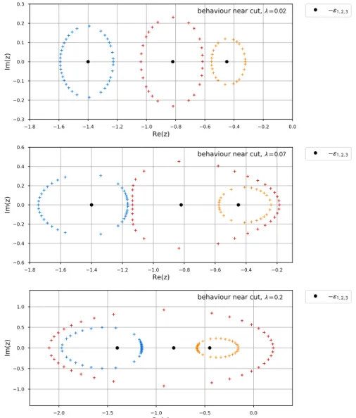
values of λoccur at which the discs swallow each other. Figure 13 shows several snapshots for d= 3.
There remains the interesting special case of %1 = %2 = .. = %d where the above picture
combines with higher-order ramification: Which circle will swallow which? We only mention that there is a multitude of interesting phenomena to be discovered.
1.8 1.6 1.4 1.2 1.0 0.8 0.6 0.4 0.2 0.0 Re(z) 0.3 0.2 0.1 0.0 0.1 0.2 0.3 Im(z) , ,
behaviour near cut, = .
1.8 1.6 1.4 1.2 1.0 0.8 0.6 0.4 0.2 Re(z) 0.6 0.4 0.2 0.0 0.2 0.4 0.6 Im(z) , ,
behaviour near cut, = .
2.0 1.5 1.0 0.5 0.0 Re(z) 1.0 0.5 0.0 0.5 1.0 Im(z) , ,
behaviour near cut, = .
Figure 13. We investigatedd= 3 with (ε1, %1) = (0.45,1), (ε2, %2) = (0.82,3) and (ε3, %3) = (1.40,2).
We see aforementioned d−1 = 2 transitions: At λ= 0.02, we observe a standard behaviour with three branch cuts. The biggest circle swallows the smallest after a certain threshold value λ1, this process is
finished atλ= 0.07. In the next transition the second-smallest circle is swallowed atλ2.
7
Conclusion
The quartic analogue of the Kontsevich model offers exceptional possibilities to study structures in quantum field theory. It is a Euclidean quantum field theory defined by deformation of a Gaußian measue. This allows on one hand to derive Dyson-Schwinger equations between
the correlation functions, on the other hand to represent these functions as a series in Feynman (ribbon) graphs. What makes this model particular is the possibility to exactly solve the Dyson-Schwinger equations in terms of algebraic or special functions. In this paper we explored the prospects of these achievements for the series of Feynman graphs and investigated transitions between different singularity types when varying the coupling constant.
After these general remarks let us be more precise about what is achieved and what is left for the future. One of the most important aspects of quantum field theory is renormalisation, which entails beautiful mathematical structures [23,11]. Renormalisation is relevant for systems with infinitely many degrees of freedom. Our model can be extended to infinitely many degrees of freedom; the Dyson-Schwinger equations relate already renormalised correlation functions. The initial non-linear Dyson-Schwinger equation has been solved implicitly [16], but in full generality. An explicit solution in terms of special functions succeeded for the 2D Moyal space (where it gives the Lambert function [25]) and for the 4D Moyal space (where it gives the inverse of a Gauß hypergeometric function [17]). In these two cases all the renormalised correlation functions of disk topology can be written down (thanks to [12]) as integral representations. Expanding them produces the familiar number-theoretical structures of quantum field theory such as multiple zeta values [8] and hyperlogarithms. We remark that the Kontsevich model itself [21] can be treated in a similar manner [15], but the expansion gives at most logarithms.
In this paper we focus on the non-planar sector of the Quartic Kontsevich Model. Although renormalisation is not needed, the limit to infinitely many degees of freedom is not yet un-derstood and needs to be studied in the future. All our results apply to a finite-dimensional approximation by N×N-matrices. We proved in [6] that all correlation functions are affiliated with a familyωg,n(z1, ..., zn) of meromorphic forms which can be explicitly computed by residue
techniques. This evaluation becomes increasingly complicated for large (g, n), but the results are remarkably structured and simple. We were led in [6] to the conjecture that theωg,n follow
blobbed topological recursion [2], i.e. the poles ofzi7→ωg,n(z1, ..., zn) at ramification points ofR
are given by a universal formula. The function R governs the solution [16,26] of the non-linear Dyson-Schwinger equation.
This paper extends [6] in expressing the coefficients of theωg,n as distinguished polynomials
in the correlation functions of the Quartic Kontevich model (see Propositions4.7and4.8). These distinguished polynomials thus evaluate to expressions much simpler than a correlation function itself (and than any of the factorially many contributing Feynman ribbon graph, see sec.5.3for their numbers). To unveil this simplicity it was necessary to transform with the inverse of the central functionR(see sec.5.2). We remark that the appearence of the distinguished polynomials is in striking contrast to the Kontsevich model [21] in which the (1+...+1)-point correlation functions themselves follow topological recursion (see [13, Chap. 6] and [15]). Moreover, the analogue ofRin the Kontsevich model is the functionx(z) =z2+const with a single ramification point at z = 0. We have shown in sec. 6 that the dependence of R on the coupling constant leads in the Quartic Kontsevich model to a very rich landscape of branch cuts with merge at critical values of the coupling constant. Of course these phenomena are only accessible because we have exact non-perturbative solutions.
After all we have seen that the Quartic Kontsevich model shares many features with honest quantum field theories: perturbative expansion into Feynman graphs, non-perturbative for-mulation via Dyson-Schwinger equations, renormalisation, evaluation into number-theoretical functions. The exact solution found step by step in [25, 16, 26, 6] permits to identify and to explore quantum field-theoretical structures which previously were hidden. Of course these structures could be special to the Quartic Kontsevich Model. Nonetheless we find it worthwhile to investigate whether something similar could be present also in realistic quantum field theories such as the Standard Model. Two questions deserve particular attention: