A Cluster-based Evolutionary Algorithm
for the Single Machine Total Weighted
Tardiness-scheduling Problem
Istv´an Borgulya
University of P´ecs, Hungary
In this paper a new evolutionary algorithm is described for the single machine total weighted tardiness problem. The operation of this method can be divided in three stages: a cluster forming and two local search stages. In the first stage it approaches some locally optimal solutions by grouping based on similarity. In the second stage it improves the accuracy of the approximation of the solutions with a local search procedure while peri-odically generating new solutions. In the third stage the algorithm continues the application of the local search procedure. We tested our algorithm on all the benchmark problems of ORLIB. The algorithm managed to find, within an acceptable time limit, the best-known solution for the problems, or found solutions within 1% of the best-known solutions in 99 % of the tasks.
Keywords: scheduling, deterministic single machine, evolutionary algorithm.
1. Introduction
The single machine total weighted tardiness problem(SMTWTP) is a scheduling problem.
In SMTWTPnjobs have to be sequentially pro-cessed on a single machine. Each job j has a processing timepj, a weight wj, and a due date
djassociated, and the jobs become available for processing at time zero. The tardiness of a job
jis defined asTj = maxf0 Cj;djg, whereCj
is the completion time of job j in the current job sequence. The goal is to find a job sequence which minimizes the sum of the weighted tar-diness given byP
i=1::n
wiTi.
The SMTWTP is anNP-hard scheduling prob-lem. Techniques which can be used to find exact optimal solution are limited to dynamic programming and branch and bound methods.
Often, instances with more than 50 jobs cannot be solved to optimality with branch and bound algorithms. Therefore, several heuristic meth-ods have been proposed for their solution 4],
5]. These include simple construction
heuris-tics, local search and metaheuristic methods. The three standard construction heuristics are the Earliest Due Date (EDD), the Modified
Due Date (MDD) and the Apparent Urgency
(AU)7]. The EDD heuristic puts the jobs in
non-decreasing order of the due datesdj. The MDD heuristic puts the jobs in non-decreasing order of the modified due datesmddj, given by
mddj =maxfC+pjdjg, where C is the sum of
the processing times of the already sequenced jobs. Finally the AU heuristic puts the jobs in non-decreasing order of the apparent urgency
auj, given by auj = (wj=pj)exp(;(maxfdj ;
cj 0g)=(kap), where ap is the average
pro-cessing time of the remaining jobs,kis the “look ahead” parameter6].
Local search algorithms repeatedly replace the current permutation π with a better sequence found in the neighborhood of π. The sim-plest local search algorithm is the lexicographic search that finds a better or the best solution in a neighborhood. We can improve the perfor-mance of the local search by choosing neighbor-hood structures. The following neighborneighbor-hood structures are customary to use:
interchange: exchange of the jobs placed at
theith and thejth position,i6=j
insert: removal of the job at theith position
More complex neighborhood structures are e.g. general pairwise interchange (GPI), adjacent
pairwise interchange (API)(this is a subset of
GPI)and dynasearch swaps(dyna). E.g. the
dy-nasearch algorithm uses dynamic programming to find the best move(transformation)in adyna
witch is composed of a set of independent in-terchange moves(Two interchanges moves are
independent if for the two moves involving posi-tioni,jandk,lhave that minfi jgmaxfk lg,
or vice versa 6]). Complex neighborhood
structure is also the variable neighborhood de-scent(VDN). In VDN we concatenate different
neighborhood e.g.interchange + insert, insert + interchangeandinsert + dyna.
We can improve performance of the local search with multi-start or iterated local search (ILS)
techniques. By multi-start the procedure run multiple, starting from different initial solu-tions, and we select the best sequence as final so-lution. A far more effective approach is to allow dependent runs by generating the new starting solution from one of the previous local optima. Such an approach, known as ILS. ILS, appears to be a very promising approach for solving the SMTWTP. A variant of the ILS, called iterated dynasearch(ILS+dyna)gives one of the best
performance results for the SMTWTP6].
Further methods for the SMTWTP are meta-heuristics. We can use e.g. simulated annealing
(SA), tabu search(TS), evolutionary algorithms (EA)and ant colony optimization(ACO). These
methods are approaching the global optimum on the analogies from physics or biology(1],5]).
We wish to enrich the scope of these heuristic methods with a new algorithm. We have aimed at developing an algorithm, which:
gives a good approximation within an
ac-ceptable time limit for recurrent tasks when using a PC (estimates the optimum within
1% of the best-known solutions); and
is easy to use with the adjustment of only a
few algorithm parameters.
In the rest of the paper, let us review the princi-ple of the new algorithm, the algorithm in detail, and its applications.
2. The principle of the new algorithm
The new method, named CE ST(Cluster-based
Evolutionary algorithm for the Single machine total weighted Tardiness problem) estimates
the global optimum by the simultaneous search for a number of local optima. It is a cluster-based evolutionary algorithm, which generates the first estimations of the local optima (
per-mutations)by grouping based on the similarity,
then it improves the results by a complex lo-cal search procedure. Further on, based on the first estimations, it periodically generates new solutions while correcting the measure of ap-proximation by local search procedures. (The
algorithm was developed by the modification of previous optimization algorithms2],3]).
The operation of CE ST can be divided in three stages: cluster forming and two local search stages. During the first stage it estimates some local optima by grouping. For problems where the neighborhood of the global optima is easy to find, it is enough to form only two clusters. But, provided the local optima hardly differ from each other, it is advisable to divide the set of permutations into more clusters. In the second stage it takes turns with a local search procedure to correct all the estimates, meanwhile it peri-odically generates new estimations of the local optima in the neighborhood of existing ones. Finally, in the third stage the algorithm further refines the estimations. Unlike in the previous stage, this time, the number of estimations is constant.
1. The first stage forms some clusters continu-ously from randomly generated feasible so-lutions. The solutions are arranged into t
clusters by their similarity and we can then accord a prototype to each cluster. The pro-totype of a cluster is always set to be the so-lution with the least objective function value, and from all possible members of the cluster only the prototype is stored. The algorithm takes the prototypes as approximations of the solution.
2. In the second stage accuracy of the proto-types is improved with a local search proce-dure that takes candidates for the improved optimum from the neighborhood of the pro-totype.
to be the VDN structure, which applies the
interchange+insert and the insert+inter-changetransformations(moves)with equal
probabilities and applies theinsertstructure in both moves at a probability of only 0.25. In selecting the prototype to be corrected, priority is given to the best, smallest objec-tive function value. The algorithm selects the fittest prototype with 0.5% probability or one of the prototypes, with 0:5=t
proba-bility(wheretis the number of prototypes).
At certain tasks this neighborhood structure is not enough for the complete run, the algo-rithm might get “stuck” at one of the local optima. To help the solution, the algorithm generates new prototypes. A new prototype is generated randomly from an already ex-isting one with an interchange + insert + interchange neighborhood structure. Thus, new prototypes can be found in the “nar-row neighborhood” of the existing ones, and, as new variants, they improve the capability and the speed of the algorithm to approxi-mate the global optimum. Thus, in the sec-ond phase new prototypes are periodically generated in the neighborhood of the exist-ing ones until a maximum number of the prototypes is completed.
3. In the third stage the solutions are further improved by the local search procedures em-ployed in the second stage. Unlike in the previous stage, this time, the number of the estimations is constant.
3. New algorithm 3.1. Algorithm as EA
The CE ST is a population-based procedure. Let us view the estimations(as permutation
vec-tors) as individuals and the generation of new
estimations from previous ones as mutations. In this case each stage can be understood as a distinct EA. In each EA a descendent is pro-duced by generations (iterations) from a
par-ent by copy making. We apply mutation, then having matched the descendant with the best cognate(or with the parent itself)we select
be-tween the parent and the descendent. We can apply the objective function as fitness function. The algorithm comprises three steady-state EAs
which produce one descendent by generations
(iterations)and select between the individuals
by means of deterministic crowding.
Let us designate the algorithm of the 3 stages as EA1, EA2 and EA3. We describe the function-ing of CE ST by means of these EAs. These are as follows:
EA1: In the first stage it creates clusters. EA2: In the second stage with a local search
it improves the quality of the solutions and periodically, in every mth iteration, increases the number of the individuals
(generates new prototypes).
EA3: In the third stage with the local search it improves the quality of the solutions.
3.2. Steps of CE ST
Introduced notations
Let us introduce the following notations:
The same population and individuals are
used with all EAs. Let p1 , p2,:::,pt be
the prototypes, that are estimations of the global optimum. Let the population of the
itth generation be denoted by P(it), and ith
individual by pi. The fitness function is
iden-tical to the Z objective function.
Measure of the similarity between the two
permutations x and z is given by H(x,z)=
1/(1+d(x,z))where d(x,z)is the Hamming
distance between the permutations.
Let us designate the random number
gener-ator as Rnd(uniform distribution on(0,1)).
Let as denote the local search procedure
Nhs(q). The procedure applies the inter
-change+insertand theinsert+interchange
transformations (moves) with equal
proba-bilities for a q permutation. In both moves theinsertstructure is applied only at a prob-ability of 0.25.
Let us denote Newind the procedure which
increases the number of the individuals.
Let us denote the pairwise interchange
pro-cedure by Swap(q). The procedure
ran-domly chooses two positions in the solution
Parameters
Five parameters affect the run of the algorithm:
tmax,t,itt,kn,manditend. Their roles one-by-one:
tmax– maximal number of the local minima
to be found.
t – number of the local minima in the first
stage to be found.
itt – a parameter of the local search. If the
number of iterations(it)reachesitt, the local
search(stage 2)begins.
m– a parameter of the local search. The size
of the population is expanded only at each
mth iteration.
timelimit – parameter for the stopping
con-dition. The procedure is finished if the run-ning time (in CPU seconds) exceeds the
timelimit.
ProcedureCE ST(tmax,t,itt,m,timelimit, opt,
optp).
* EA1 ******************************** it:=0, glob:=1,kn =100. /* Initial values.
Let pi 2 Π(n) (i=1,...,t), P(it) fp1 ::: ptg.
Compute Z(p1) ::: Z(pt).
Repeat
i:=t*Rnd]+1, q:=pi. /* New descendent
Forj:=1to4doSwap(q)od. /* Mutation
Compute Z(q).
Let H(q,pz)=maxjH(q,pj);j,z2f1,2,...,tg.
IfZ(q)<Z(pz)thenpz:=qfi. /* Selection
it:=it+1, P(it)P(it-1).
untilitt<it.
*EA2********************************* Repeat
Repeat
If0.5<Rndtheni:=glob
elsei:=t*Rnd]+1fi.
q:=pi /* New descendent
Nhs(q). /* Mutation
Compute Z(q).
IfZ(q)<Z(pi)thenpi:=qfi./* Selection
it:=it+1, P(it)P(it-1).
If mod(it,m)=0thenNewindfi.
untilmod(it,kn)6=0.
Let Z(pi)=minjZ(pj),i,j2f1,2,...,tg, glob:=i.
opt=Z(glob): optp=pglob
If“running time” >timelimitthen exitfi. untilt<tmax.
* EA3******************************* Repeat
Repeat
i:=t*Rnd]+1
q:=pi. /* New descendent
Nhs(q). /* Mutation
Compute Z(q).
IfZ(q)<Z(pi)thenpi:=qfi./* Selection
it:=it+1, P(it)P(it-1).
untilmod(it,kn)6=0.
Let Z(pi)=minjZ(pj), i,j2f1,2,...,tg, glob:=i.
opt=Z(glob): optp=pglob
until“running time” <timelimit.
*********************************** exit
end
3.3. Details of Implementation
When describing the algorithm, some heuristic solutions and the shortcuts of the computations were not described. Let us see them now one-by-one.
Initial population
In our implementation the initial population is generated by the EDD heuristic. First we gen-erate a permutation, which is the solution of the EDD, and second, we generate all individual of the initial population from this permutation with 4interchangemoves. With the help of this initial population the algorithm can converge faster.
Heuristic in the neighborhood structure
We use the rule of the EDD heuristic also in the neighborhood structure. The first move in theNhs procedure uses the positions i,j. Our algorithm looks for a randomi,jposition at the probability of 0.9 so asdj <diis true. It tries to
find an appropriatei,j position only 10 times, and if it does not succeed, this heuristic rule is skipped.
Speeding-up the computation
After each application of the Nhs procedure only one or two parts of the series is changed, all the other positions of the actual permuta-tion remain unchanged. So only those partial sums of the total weighted tardiness that were changed after applying the Nhs have to be re-calculated. Naturally, this shortcut can be used only if we keep theck,wktk(k=1 ::: n)
vec-tors calculated earlier and we can use them in the calculation of the new function value. To speed up the calculation, the algorithm is stor-ing theck,wktk (k=1 ::: n)vectors for each
individual.
4. Test Results
Test problems
We have tested the CE ST with the benchmark set of the randomly generated instances, avail-able via ORLIB athttp://www.ms.ic.ac.uk/
info.html. The benchmark set comprises
in-stances with 40, 50, and 100 jobs. In each three sets there are 125 instances. For the 40 and 50 job instances optimal solutions are known, while for the 100 job instances only the best-known solutions are given.
Parameter selection
To achieve a quick and accurate solution we need appropriate parameter values. Studying some of the more complex problems of the benchmark set we analyzed how parameter val-ues were affecting the convergence, finding of the global optimum and the speed of the calcu-lation.
So we analyzed the number of prototypes, which should be used in CE ST to achieve a good trade-off between the probability of finding best-known solutions and the necessary run-time to do so. In general, the best behavior has been obtained with a number of prototypes between 5 and 30. For a too small number of prototypes, some optimal solutions are found rather fast, but with increasing the run-time often CE ST with a larger number of prototypes the achieves higher probabilities of finding optimal solutions. So for test problems the number of prototypes of 30 was found appropriate(tmax =30).
As a next step, we analyzed the influence of the second stage on the run-time and on the con-vergence. We concluded that both the speed of
convergence and the quality of the result are im-proved if we start the 2nd stage with a lower ini-tial number of clusters and broaden this number by adding a new element to the population every time after some thousand iterations. But, in this situation, it is also true that a larger number of clusters achieves higher probabilities of finding optimal solutions. The speed of convergence is influenced by the frequency of broadening of the population, too. We found that the con-vergence is more successful if the population is broadened relatively slowly, after some thou-sands of iterations, than if we broaden it more quickly, after each 100-200 iterations. We con-cluded that an initial number of clusters of 10
(t = 10)and a broadening at every 5000
itera-tions(m = 5000)was observed to be optimal
on the benchmark sets.
Finally, we studied the number of iterations of the first stage. We found the first stage to be necessary, because forming the first clusters is beneficial on the accuracy of the results, it usu-ally decreases the scatter of the result. However, 1-2 hundreds of iterations are enough for form-ing the clusters(this is the most time consuming
part of the run of the algorithm).
The following parameters were used at the test problems: t = 10, tmax = 30, m = 5000,
itt = 100. Run time was set to 6, 12 and 80
seconds for the 40, 50 and 100 job instances, respectively.
Comparative results
As for comparison, we chose the multi-start ver-sion of the TS, SA (the number of starts is
5) and the iterated dynasearch (ILS-dyna) of
Crauwels, Potts and Van Wasserhove (1998).
For the comparison 5] and 6] included data
of sufficient details, some of which we used.
(We couldn’t include the ACO method 1] in
the range of methods chosen for comparison, because data including sufficient details were not available.)
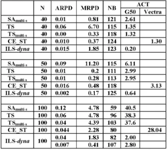
The comparison was encumbered by the use of various programming languages, operating systems and computers. Only one appropriate aspect of comparison could be found, namely the average relative percentage deviation of the solution from the best known solution, so our table of comparison (Table 1) is based on the
results of comparable accuracies. (Our CE ST
Vectra with 128 MB RAM, and the program was written in Visual Basic and run under Windows 2000 professional. The TS and ILS-dynasearch programs were written in C and run using an HP 9000-G50 computer).
Table 1.Comparative results.
We compared average results: for all the four algorithms we ran each problem(or others ran
each problem)10 times, and the average results
are shown. We compared performance of the various algorithms on the basis of the follow-ing statistics: the average relative percentage deviation of the solution from the best known solution (ARPD); the maximum relative
per-centage deviation of the solution from the best known solution(MRPD); the number of the best
known solution values found out of 125(NB);
the average computation time in second(ACT)
on a HP 9000-G50 (G50) or on a HP Vectra
VL800(Vectra).
Reviewing the results we can conclude that the ILS-dynasearch algorithm yielded the best re-sults. It reached the specified accuracy in the shortest time, and in more cases it was the one that found the best known solutions.
According to the statistics the results of the CE ST are mostly between the results of the multi-start TS and the ILS-dynasearch. If we focus on the details of the run, we see that the CE ST managed to find within the acceptable time limit the best-known solution for the prob-lems, or found solutions within 1% of the best-known solutions in 99% of the tasks. This result
can be specified further: the CE ST found solu-tions within 0.1% of the best-known solusolu-tions in 90% of the tasks.
Considering that the TS and ILS-dynasearch are the most effective methods of SMTWTP, we can conclude that the CE ST belongs to the best available methods, too.
5. Summary
We can conclude that the CE ST was success-fully tested with different kinds of SMTWTP. The method solves the usual test problems at a very good accuracy and performance. Compar-ing the results with other heuristic methods, we can conclude that the CE ST belongs to the best methods of this problem scope. The build-up of the method, especially the possibility of broad-ening the 2nd stage population, allows quicker convergence in comparison to former methods. In this field our method has possibilities com-parable to the ones of the ILS technique. We still did not use up the possibilities of the method: for example, there is a possibility of speeding up the convergence. Changing to the
C programming language instead of the cur-rent one, or realizing further speed-up possibili-ties would make computation time even shorter, which would allow improved accuracy, too.
Acknowledgments
The Hungarian Research Foundation OTKA T 030861 supported the study.
References
1] BESTENM., STUTZLE¨ T., DORIGOM., Ant Colony
Optimization for the Total Weighted Tardiness Prob-lem. In: Schoenauer M. et al. editors, Parallel Problem Solving from Nature — PPSN VI. Lecture Notes in Computer Science1917, Springer-Verlag Berlin 2000, pp. 611–620.
2] BORGULYA I., Constrained optimization using a
clustering algorithm.Central European Journal of Operations Research.8(1)2000. pp. 13–34.
3] BORGULYA I., A Cluster-based Method for the
4] BRUCKERP., HURINKJ., Complex Sequencing
prob-lems and local search heuristics. In: Osman IH, Kelly JP. editors, Metaheuristics: Theory and Ap-plications, Kluwer Academic Publishers, Boston, 1986. pp. 151–166.
5] CRAUWELSHAJ., POTTSCN., VANWASSENHOVE.,
Local search heuristics for the single machine total weighted tardiness- scheduling problem.INFORMS Journal on Computing101998. pp. 341–350. 6] CONGRAMRK., POTTSCN.,VAN DEVELDE, An
it-erated dynasearch algorithm for the single-machine total weighted tardiness scheduling problem. Tech-nical report. Faculty of Mathematical Studies, Uni-versity of Southampton, December(1998).
Received:June, 2002
Accepted:September, 2002
Contact address:
Istva´n Borgulya University of P´ecs R´ak´oczi ut 80 7621 P´ecs, Hungary e-mail:[email protected]