Towards a Software Tool Supporting
Urban Decision Makers in Locating
and Sizing the Household Garbage
Accumulation Points Within Cities
Paolino Di Felice
Department of Industrial and Information Engineering & Economics, University of L’Aquila, L’Aquila, Italy
Locating and sizing garbage bins for the separate accu-mulation of household solid waste within urban areas is of primary interest for the local administrations that so far lack adequate IT support. The paper highlights the versatility of a method for solving such a problem, which involves both standard and geographic data. Implemen-tation of the proposal, centered around a spatial database, goes in the direction of developing a supporting software tool to the officials responsible for the management of municipal solid waste. They are offered a dual-mode display of the results: one tabular (the standard format featured by relational databases)and the other based on the metaphor of geographic maps, the latter being partic-ularly useful in capitalizing on the spatial component of the problem.
Keywords: solid waste, garbage accumulation point, garbage bin, algorithm, integrated spatial and descriptive data, SQL, decision support system
1. Introduction
“Managing solid waste (SW) well and afford-ably is one of the key challenges of the 21st century, and one of the key responsibilities of a city government”(UN-HABITAT, 2010). The quality of waste management services is a good indicator of a city’s governance. The way in which waste is produced and discarded gives us a key insight into how people live. In fact, if a city is dirty, the local administration may be considered ineffective or its residents may be accused of littering.
The major types of urban SW are residential and commercial. Households are the high-est producers of municipal waste(EEA, 2013).
Damghani et al.(2008)report that in Tehran, the capital of Iran, the contribution of the household SW to the total municipal SW is around 62%. A similar estimation about the Americans’ pro-duction of residential SW is reported in (US EPA, 2010).
Tchobanoglous et al.(1993)categorize the ac-tivities of a municipal SW management sys-tem as a six steps procedure: waste generation; handling, separation, storage, and processing at the source (in the following briefly called ac-cumulation); collection; transfer and transport; separation, processing and transformation; and disposal.
In Italy, nowadays, SW is accumulated us-ing two complementary methods. For many years, the municipalities have spread on the ma-jor crossroads in the towns large-sized garbage bins (GBs). Daily, households put their SW in these public containers, while, cyclically, municipality-owned machines take away the SW from them. A more recent method con-sists of providing families with much smaller GBs and municipal workers collect the garbage door-to-door. So far, the first method covers the largest waste disposal production. That is why this study refers to such a scenario.
From the citizens’ point of view, SW accumula-tion and collecaccumula-tion are among the most visible urban services. If properly implemented, they contribute:
− to develop the culture of urban cleanliness; − to protect municipal workers dealing with
the collection and transportation of infec-tious waste materials(Miyazaki et al., 2007); − to protect the health of pets (they regularly visit GBs looking for food residues, with the tangible risk of getting sick)and, therefore, they contribute to protect the health of resi-dents, too;
− to keep high the market value of the apart-ments in the area;
− to get high residents’ satisfaction. In fact, the effectiveness of garbage accumulation and collection is a variable largely used in the studies investigating the satisfaction of individuals living in the urban areas, e.g.,
(Felix & Garcia-Vega, 2012).
Unfortunately, spatial distribution of the garbage accumulation points(GAPs)inside towns does not take the needs of local residents into account in terms of the quantities of waste produced and the distance from their dwelling (Parrot et al., 2009). That induces the following two side ef-fects: a) often the GBs are full and, in those cases, the citizens’ decision is to leave the bags of garbage outside the GBs; b) when the dis-tance to the closest GB is long, households tend to dispose the domestic waste in open areas. Similar concerns about inconvenient location of the GAPs are expressed by Zia & Devadas
(2008).
In our opinion, the only way to overcome those limits is to provide local administrators with an ad hoc software tool assisting them during the GBs allocation phase. This work was meant to give a contribution in the direction of develop-ing a software tool of this type.
The tool has to be developed on top of a gen-eral method that solves “correctly” what in the remainder of the paper we call the solid waste accumulation problem(SWAP). Here, correctly means to come to a location of the GAPs in the urban territory, linked to the distance from the house of the citizens; moreover, the number of bins per GAP has to be adapted to the amount of waste “locally” produced by the citizens. Do-ing so, both drawbacks mentioned above should disappear.
1.1. Related Work
A huge amount of research has been done about facility location problems in the field of oper-ational research; for a survey see (ReVelle & Eiselt, 2005). However, as remarked by Ghi-ani et al. (2012), contrarily to other location problems in the context of urban waste man-agement, the SWAP has received little attention in the literature and only quite recently.
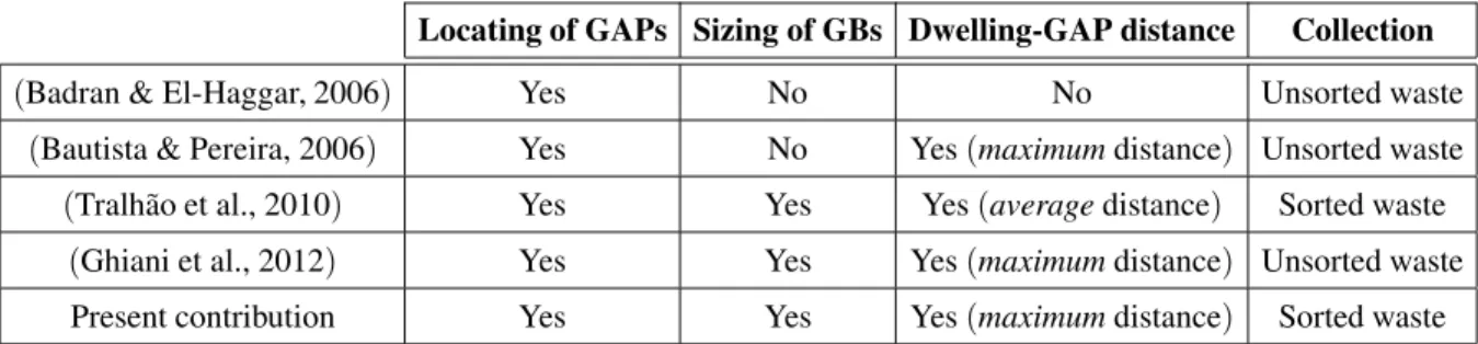
The unique papers pertinent to the topic are listed and compared in Table 1. The second column in Table 1 tells us that all the papers solve the problem of locating the GAPs in the urban territory to be served. Their common ob-jective is to minimize the number of GAPs in order to reduce: a)the initial cost of buying the GBs, b)the collection time, and, finally c)the negative visual impact caused by the presence of the GBs near residential buildings.
The third column shows that only the last three papers also compute the sizing of GBs inside each GAP, while the first two do not.
The fourth column tells us about the way those papers take into account the distance between the dwellings and about what in this study we
Locating of GAPs Sizing of GBs Dwelling-GAP distance Collection
(Badran & El-Haggar, 2006) Yes No No Unsorted waste
(Bautista & Pereira, 2006) Yes No Yes(maximumdistance) Unsorted waste
(Tralh˜ao et al., 2010) Yes Yes Yes(averagedistance) Sorted waste
(Ghiani et al., 2012) Yes Yes Yes(maximumdistance) Unsorted waste
Present contribution Yes Yes Yes(maximumdistance) Sorted waste
call the reference GAP, that is, the GAP clos-est to the houses. (Badran et al., 2006) ignore the issue, while(Tralh˜ao et al., 2010)minimize the average distance from dwellings to the ref-erence GAP. The remaining three papers take the distance dwelling-(reference)GAP within a fixed maximum threshold. It is fundamental to guarantee that each family has, at a “suitable” distance, a GAP and this assures an adequate quality of the service to all residents in the area. Relevance of this issue has been pointed out clearly in numerous studies about the “qual-ity of life”, e.g., (Felix & Garcia-Vega, 2012). Quality of the service of accumulation and col-lection of the household waste is perceived as relevant by citizens for two reasons. Because they support this service by paying taxes and, therefore, it is quite obvious that they have ex-pectations reqarding the quality of the returned service, and, moreover, because of the growing public concern about environmental preserva-tion.
The last column in Table 1 specifies whether the SW is accumulated/collected in a sorted or unsorted way.
Ghiani et al. (2012) give two alternative solu-tions of the SWAP: the first adopts an integer programming model, while the second adopts a two-phases heuristic approach. They intro-duced the latter approach because the complex-ity of the integer programming model makes it very difficult to be solved optimally within a reasonable time by means of a general purpose solver. The method we propose in this paper bears a likeness to the heuristic approach by Ghiani et al. (2012), with which it shares also the motivation of finding a good solution of the SWAP in a short computational time.
Ghiani et al. (2012) start from a given set of GAPs located at a known position inside the city and return the minimum number of reference collection sites to be allocated, chosen among the initial candidates. In our approach, on the contrary, the reference GAPs may be located at any point of the city roads (same assumption as in Bautista & Pereira, 2006)and their num-ber and position result from the elaboration of a method determined by the “urban geography” of the dwellings to be served.
The remainder of the paper is structured as fol-lows. Section 2 defines the SWAP inside mod-ern towns and lists our notations. Section 3
focuses on two algorithms that together provide a general solution of the SWAP by integrating spatial and descriptive data. The first algorithm determines the location of the GAPs in the urban territory to be served, while the second allocates the number of bins to each GAP. The position of the GAPs is set by taking into account the distance from the house of the citizens, while the number of bins is adequate to the amount of litter produced “locally” on daily basis. Such two-phases method has been introduced in(Di Felice, 2013). The algorithms strictly refer to the accumulation of the residential SW, but they can be easily adapted to other types of litter
(e.g., the commercial SW). Section 4 touches on a way to implement the two algorithms in terms of open source software, while Section 5 reports about a pilot study applied to a political district of the town of L’Aquila(central Italy), whose results are presented and discussed in Section 6. Those three sections show a simple and effective way to implement the theory using the technology of the spatial database manage-ment systems(SDBMSs), and, more important, the versatility of the proposed solution from the point of view of those responsible for munic-ipal SW management who, in fact, is offered a dual-mode display of the results: one tab-ular (typical of relational databases) and the other based on geographical maps, this latter particularly useful to capitalize on the spatial component of the SWAP. Together, these two operational modes provide a very effective as-sistance to decision makers. Section 7 focuses on the flexibility of the first algorithm in the allocation of dwellings to the GAPs and on the positive effects of such a feature. Section 8 lists a few SQL pattern queries that make explicit the analysis on demand dimension embedded in the SDBMS-centric implementation we carried out. In fact, by querying the spatial database(SDB), it is possible to extract a lot of extra information from the SDB not easily obtainable in any other way. Section 9 ends the paper.
2. The Solid Waste Accumulation Problem
and V2 represent the GAPs. To each arc a numerical value (distij)can be associated, rep-resenting the distance between dwelling i and its potential reference GAP (j). Ghiani et al.
(2012) start from a given set of GAPs located at known position inside the city, therefore they have V1, V2, anddistijas inputs. Contrarily, we
ignore the geographical position of the vertices in V1(and hence the valuesdistij), because, as already noted, in our case the GAPs may be located at any point of the city roads.
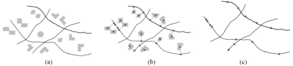
At a less abstract level, the SWAP inside mod-ern towns can be formulated as follows: given the set of houses and public roads (the spatial data)being a part of an urban area(Figure 1a), the goal is to compute the location of the GAPs in the area as well as sizing the number of bins. Further relevant data of the problem (they all together give rise to thedescriptive data)relate to the type of waste to be stored in the GAPs, capacity of the GBs, the frequency of emptying the GBs of various types, the number of inhabi-tants in each house in the area to be served, and their per capita daily production of SW.
We solve the SWAP under the following con-straints:
a) the GAPs have to be placed on the public roads;
b) every house must have its reference GAP at a distance(measured along the public roads)
not greater than a predetermined value; c) the number of bins for the different types
of waste in each GAP must be allocated ac-cording to the daily production of household waste of the district.
Notations
Hereafter we use the following notations: District is the urban area to be served with GAPs,
R={r1,r2, . . . ,rR} is the set of public roads
crossing theDistrict. The generic element ofR,rj, is a triple<id,name,the geom>
whose values, in sequence, denote the uni-que identifier of the road, its name, and the geometry modeling its shape,
H={h1,h2, . . . ,hH}is the set of houses located
inside the District. By house we mean a building having a certain shape on the ground. We do not care about the number of floors composing each building, while the number of people living in it is relevant. The generic element of H, hj, is defined
by the tuple < id, road id, num, density, the geom, the geom c, the geom h > who-se values, in who-sequence, denote the unique identifier of the house, the unique identi-fier of thereferencepublic road(that is the road that specifies the building’s address), the house number, the number of occupants in the dwelling, the geometry of its layout
(i.e., a polygon), the simplified geometry of the dwelling (i.e., the centroid of the polygon), the geometry of the projection of the centroid of the dwelling on the ref-erence public road. Figure 1b shows the geometry of the layout of the houses, their centroid and the projection of the centroid on the reference road. From here on, when talking about dwellings, we always refer to the projection of their centroid on the refer-ence road; therefore, the scene in Figure 1a is replaced with that in Figure 1c,
GB = {gb1,gb2, . . . ,gbGB} is the set of the
different types of GBs that are part of each GAP. In the study, we take into account the following five types: glass,plastic, pa-per, organic, and unsorted, but the solu-tion method is general, so it can be adapted to work under different assumptions. The
generic element of GB, gbj, is defined by
the tuple<id,type,capacity,collection>
whose values, in sequence, denote the unique identifier of the GB, its type, its capacity (m3), and the frequency of
col-lection (days) from municipality’s work-ers. For example, the tuple<1, glass, 1.8, 7 >specifies that the GB is of type glass, it has id 1, capacity 1.8 m3, and weekly frequency of collection,
GAP= {gap1,gap2, . . . ,gapGAP} is the set of
GAPs to be dislocated in theDistrict. The generic element ofGAP,gapj, is defined
by the tuple<id,the geom,road id,glass, plastic,paper,organic,unsorted,rs,hs>
whose values, in sequence, denote the unique identifier of the GAP, its coordi-nates, the id of the public road wheregapj
is located, the number of GBs for glass, plastic, paper, organic, and unsorted, and, lastly, the total number of residents and houses that the GAP is able to serve, housesServedBy aGAP[]is an array of sets data
structure having a number of components equal to the cardinality ofGAP. The com-ponent housesServedBy aGAP[k]stores the
(sets of)identifiers of the houses served by the GAP having identifier equal tok,
dailyGlass, dailyPlastic, dailyPaper, dailyOr-ganic, and dailyUnsorted denote, in se-quence, the per capita daily generation(in
m3) of the five different types of SW we refer to in the paper,
Distancedenotes the value of the maximum dis-tance between each house and the reference GAP(that is the GAP closest to the house). All identifiers are positive integers starting from one. Moreover, in the algorithms we are go-ing to present, we use, for brevity, the nota-tion “record name.field name” linking a com-posite variable(record)to one of its parts(field). Therefore, for example, gapj.id denotes the
identifier of the elementgapjof setGAP.
3. A Strategy to Solve the SWAP
The solution of the SWAP is obtained in two stages via the algorithmsLocatingOfGAPsand
SizingOfGAPs to be invoked in sequence. As mentioned in the Introduction, this schema has analogies with the two-phases heuristic approach proposed by Ghiani et al.(2012).
LocatingOfGAPstakes as input the setsHand R, and the value ofDistanceand returns the set GAP and the data structure housesServedBy aGAP[] to be used as input of the algorithm
SizingOfGAPs. After the set GAP is initial-ized, theFOR EACHloop is activated. It runs until all the public roads inRhave been visited. The visit of the generic road(Line3)is devoted to locate the position where the GAPs have to
Algorithm LocatingOfGAPs
Input: H,R,Distance
Output: GAP and housesServedBy aGAP[]. The generic tuple ofGAP has value: < id, geom, road id, NULL, NULL, NULL, NULL, NULL, NULL, NULL >
Method:
1. SetGAPto the empty set. 2. FOR EACHrinR
3. move along r and locate on it the GAPs according to the constraint that the distance
(reference)GAP-house is at most equal toDistance. 4. AddtoGAPallthe GAPs located alongr.
5. Letgapbe one of such GAPs and Hrbe the set of the identifiers of the houses onrserved by it. gap.iddenotes the identifier ofgap.
6. Set gap.geomto the position of gaponr. Setgap.road id = r.id. Set toNULLthe
remaining values of the record aboutgap.
7. Addthe identifiers in Hrto the set housesServedBy aGAP[gap.id].
8. Explorethe neighbourhood ofgap.geomto identify further houses(if any)that do not have
ras the reference road, but that can be served bygapsince it is distant less thanDistance
from them. Let H* be the set of the identifiers of those houses. 9. Addthe identifiers in H* to the set housesServedBy aGAP[gap.id].
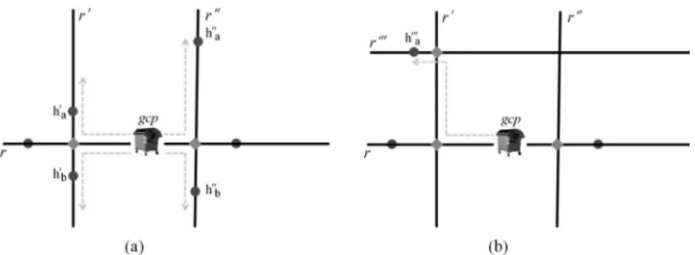
Figure 2.Dwellings close to the GAPgap(schematically represented by one of the GBs being part of it)
located on roadr, but having as reference road one different fromr.
be allocated. The decision takes into account the value of the geometry of the projection of the centroid of the dwellings havingras the ref-erence road(the fieldthe geom hof Section 2; see also Figure 1c) and the value ofDistance. Each time a position is found, the algorithm sets the values of the fields gap.id, gap.geom,
andgap.road idof the record referring togap,
while the remaining fields are set toNULL(Lines
5 and 6). Line 7 copies the identifiers of the dwellings located along r and served by the GAPgapin the set housesServedBy aGAP[gap. id]. All those dwellings havegapas the
refer-ence GAP.
The purpose of Line 8 is to identify further houses (if any) that do not have r as the ref-erence road, but that can be served by gap
since it is distant less thanDistancefrom those dwellings. There are two possible situations to be investigated. The first one(Figure 2a)is that
of houses that lie on roads that intersectrnear to the point where is positionedgap. In the figure,
ris intersected by roadsr’ andr” at the points marked as diamonds. By hypothesis, H*={h’a,
h’b, h”a, h”b}, i.e., the dwellings h’a, h’b, h”a
and h”bare considered to be served bygap. The
second situation(Figure 2b)is about houses that lie on roads different either fromr or from the streets that intersectr, but still they are close to
gap. In Figure 2b, by hypothesis, house h”’a,
located on the roadr”’, is distant less than Dis-tancefromgapand, therefore, it can be served
by such a GAP. In summary, H*={h’a, h’b, h”a,
h”b,h”’a}. Also the dwellings in H* havegap
as the reference GAP. At the end of each iter-ation, the set housesServedBy aGAP[gap.id]
collects the identifiers of all the roads in H, served bygap, independently of their reference
road.
Algorithm SizingOfGAPs
Input: H,GB,GAP, housesServedBy aGAP[],dailyGlass,dailyPlastic,dailyPaper,
dailyOrganic, anddailyUnsorted
Output: GAPupdated
Method:
1. FOR EACHgapinGAP
2. CopyhousesServedBy aGAP[gap]into HS
3. Setgap.rsequal to the sum of valueshj.density(j=1, 2,. . ., |HS|), wherehjbelongs to HS 4. Setgap.hsto |HS|
5. Computethe number of different types of GBs that make up the GAPgapby taking into account:
a)their capacity(i.e.,gb.capacity),
b)the daily per capita generation of SW of different typologies from the
gap.rsresidents, and
c)the periodicity of waste collection of different typologies(i.e.,gb.collection)
6. UPDATEthe fieldsglass,plastic,paper,organic,unsortedofgap
A more detailed version of the algorithm Lo-catingOfGAPs may be found in (Di Felice, 2013).
SizingOfGAPsupdates the values of the records of the set GAP relatively to the fields left to
NULL by LocatingOfGAPs. The algorithm
re-peats, for each GAP in GAP, the following steps. Letgapbe the generic GAP. Initially, the
content of the set housesServedBy aGAP[gap],
i.e., all the dwellings served by gap, is copied
into the variable HS (HouseServed). Then
(Line 3), the total number of citizens that gap
can serve is calculated. This is done by adding togap.rsthe number of inhabitants in each of
the houses present in HS. Line 4 sets the field
gap.hs to the value of the number of houses
served bygap. The next step(Line5)computes
the number of GBs of the five types taken into account in our study. For example, the number of GBs for the glass is calculated as follows:
gap.glass=(gap.rs*dailyGlass*glass. collection)*0.85/(glass.capacity).
Set gap.rs=165, dailyGlass=0.005 m3, glass.co-llection=7, and glass.capacity=1.8 m3, it fol-lows that gap.glass = 2.73 that is rounded up to 3. The value 0.85 introduces a margin of caution in estimating the number of GBs. Ob-viously, this threshold can be changed as desired or eliminated altogether.
The final step of the sizing algorithm consists of updating the fields glass,plastic, paper, or-ganic,unsortedofgap.
4. Implementation
The implementation of algorithms LocatingOf-GAPs and SizingOfGAPswas achieved in two
steps. The first step was about the design of a SDB and its subsequent implementation in Post-greSQL/PostGIS, followed by loading in it the spatial and descriptive data necessary to solve the SWAP. Then, we coded the two algorithms in the language PL/pgSQL(http://www.post
gresql.org/docs/9.1/static/plpgsql.html)
as user defined functions(UDFs).
The SDB is composed of the following five ta-bles(the primary keys are underlined):
road (id, name, the geom);
house (id, road id, GAP id, num, density, the geom, the geom c, the geom h);
GAP (id, the geom, road id, glass,
plastic, paper, organic, unsorted);
GB (id, type, capacity, collection);
GAP GB (GAP id, GB id);
road,house,GAP, andGBstore, in sequence, the
elements in the setsR,H,GAP, andGB.
The above relational schema comes from the conceptual schema of Figure 3, where for each entity the identifying attribute and the (min, max) participation constraints in the relation-ships are shown.
The implementation of algorithms LocatingOf-GAPs and SizingOfGAPs as UDFs has been greatly facilitated by the use of the following PostGIS functions: ST Area(),ST Centroid(), ST Distance(),ST Intersection(),ST Inter-sects(), ST Length(), ST Line Interpolate Point(),ST LineMerge(),ST Line Locate Po-int(),ST Line Substring(), AddGeometryCo-lumn().
The computation of the set H* (Line 8, algo-rithmLocatingOfGAPs)with regard to a given GAP, let say gap, requires the visit of all the
routes that lead to dwellings not far away from
gapmore thanDistancemoving along the
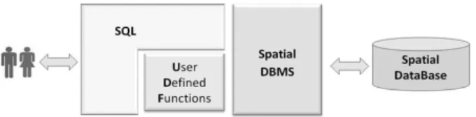
pub-lic roads. This action is carried out by visiting in depth the graph having as nodes the end points of the roads in R, the crossings between the roads in R, the houses in H, and the GAPs in GAP and, as arcs, segments of the roads inR delimited by pairs of nodes. The distances be-tween pairs of points situated along the roads are computed as the shortest path between them. The software architecture of the implementa-tion (Figure 4)offers two major benefits: first of all, it relies on the SDBMS technology which
Figure 4.The software architecture of the implementation.
allows to take advantage of the expressiveness of the SQL language for querying the SDB( ex-pressiveness that can be further improved by invoking either some of the implemented UDFs or the built-in functions); second, it makes ex-clusive use of open source software, a choice today in a sense mandatory for the municipal administrations chronically short of cash flow.
5. Study Area and Input Datasets
The Cansatessa district
As study area, about 7 km2, we refer to the
po-litical district of Cansatessa, part of the town of L’Aquila(the capital of the Abruzzo region; central Italy). In the district, 1464 inhabitants, are distributed in 226 buildings (Figure 5, left side), while there are 17 public roads.
L’Aquila municipality is responsible for the management of the SW life cycle in all the dis-tricts, including Cansatessa. Figure 6 shows the five categories of large-sized GBs currently adopted, while their capacity is given in Table 2.
Figure 5.A Google view of the district of Cansatessa(42◦23’ 0” N, 13◦20’ 35” E), L’Aquila(Italy) (left side). The public roads and the houses of Cansatessa extracted from a shape file of the Abruzzo region(right side)
and displayed by using QGIS.
According to the last available regional report
(OBRA, 2011), this method of accumulation in the municipality of L’Aquila covers 83.57% of the total waste generated by the residents.
Types of
household SW Frequency ofcollection the GBs (mCapacity of3)
Organic Each 3 days 2.4
Plastic Each 3 days 2.4
Paper/cardboard Each 5 days 3.3
Glass Each 7 days 1.8
Unsorted Daily 2.4
Table 2.The capacity of the different types of GBs adopted in the municipality of L’Aquila and the periodicity of collection by means of municipal
garbage trucks.
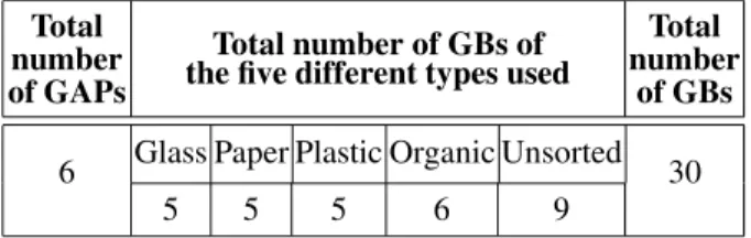
Table 3 summarizes the current situation in the district of Cansatessa in terms of GAPs and GBs.
Total number of GAPs
Total number of GBs of thefive different types used
Total number
of GBs
6 Glass Paper Plastic Organic Unsorted 30
5 5 5 6 9
Table 3.GAPs and GBs in Cansatessa.
The datasets
The datasets concern both spatial and descrip-tive data.
The spatial data
The spatial data concerning public roads and houses of Cansatessa were extracted (in the ESRI shape format)from the Regional Numer-ical Map at the 1-5000 scale provided by the Abruzzo Region(http://www.regione.abruz zo.it/xcartografia/). Figure 5(right side)
shows the content of this shape using QGIS. These spatial data are sufficient to feed the al-gorithmLocatingOfGAPs.
The descriptive data
The situation is much more complex with re-gard to the descriptive data necessary to feed the algorithmSizingOfGAPs. The data we are talk-ing about concern the number of people livtalk-ing inside the dwellings and their per capita daily
production of SW of different types. Having reliable data at this level of detail is not trivial because, as stated in recent field studies (e.g., Lebersorger & Beigl, 2011), these values are dependent on many variables, including time of the year, weather, household income, size of their homes, type of heating system in the apartments, etc.
Over time volatility of data is another critical issue against the acquisition of reliable data to feed the algorithmSizingOfGAPs. In fact, what we are witnessing is that, partly because of the legislative pressures that exist in all European countries, the quotas of separate collection of municipal SW increase from year to year. By contrast, the data available date back to several years ago. For example, the latest study within the Abruzzo region (OBRA, 2011) reports the data from 2009.
Last practical difficulty, but certainly not the least, comes from the fact that there is no unique transformation ratio between the weight of SW
(expressed in kg) and its volume, while it is precisely from these data that we need to solve the SWAP properly, given that the capacity of the GBs is expressed in m3. Nor are there any
studies on the subject(as far as we know)from which to draw them. The relevance of this is-sue has been stressed recently by Hoornweg & Bhada-Tata (2012), where we read: “Al-though waste composition is usually provided by weight, waste volumes tend to be more im-portant, especially with regard to accumula-tion”.
All the above mentioned issues have a direct im-pact on the outcome of the sizing stage. There-fore, it is correct to say that the goodness of the estimates provided by the method proposed in Section 3(as well as any other similar method)
largely depends on the accuracy of the input data.
In the present pilot study, given the impossibil-ity of making use of updated data on a local basis, we adopted “synthetic” data (Table 4). The 2nd column sets the number of residents served by a specific GB before it becomes full at 85%, according to the weekly periodicity of collection of the SW by the municipal workers. So, for instance, from Table 4 we learn that a GB of Glass type can serve at the most 120 people within seven days.
Category of
household SW Number of residentsserved by one GB
Organic 80
Plastic 130
Paper/cardboard 100
Glass 120
Unsorted 210
Table 4.The descriptive data used to run the algorithmSizingOfGAPs.
6. Results and Discussion
Locating of the GAPs
First campaign of experiments
As first set of experiments, theLocatingOfGAPs
algorithm was run varying the value of the Dis-tanceparameter as follows: 50, 100, 150, 200, 250, 300, 500(meters). The findings in(Parrot et al., 2009) advise against going further. The seven experiments were repeated three times changing the order in which the roads in the set R were visited. Table 5 collects the results of the campaign of experiments.
Number of GAPs
Distance (m)
Order no.1 of visit of the roads
Order no.2 of visit of the roads
Order no.3 of visit of the roads
50 41 41 41
100 27 27 27
150 22 20 21
200 16 17 18
250 13 14 13
300 9 10 9
500 5 6 5
Table 5.The results of the first campaign of experiments.
As it was predictable, the number of GAPs de-creases as the value ofDistanceincreases. But Table 5 also shows that the number of GAPs is affected by the order in which the first algo-rithm visits the public roads. This dependence is deepened below.
Second campaign of experiments
The second campaign of experiments consisted of runningLocatingOfGPAsfor the same seven values of the parameterDistanceas in the first campaign of experiments, but in two extreme situations: for descending (ascending) values of the length of the roads (Table 6). In other words, in the first seven runs, the algorithm lo-cates the GAPs first on the public road 1493m long, then on that 1046m long, and so on. While in the next seven runs it locates the GAPs first on the public road 80m long, then on that 85m long, and so on.
# Road id Length (m)
1 15 1493
2 17 1046
3 4 632
4 5 400
5 9 359
6 14 270
7 1 242
8 3 217
9 11 206
10 6 188
11 2 187
12 7 163
13 13 146
14 10 114
15 8 111
16 16 85
17 12 80
Table 6.The 17 public roads in Cansatessa, listed for descending value of their length.
Table 6 was built by querying the SDB by means of the following spatial query:
SELECT id, round(ST Length(ST LineMerge
(the geom))::numeric) AS Length
FROM road
ORDER BY ST Length(ST LineMerge(the geom)) DESC
Distance
(m) descending orderRoads visited in ascending orderRoads visited in
50 41 41
100 25 27
150 18 23
200 12 19
250 8 15
300 7 10
500 4 6
Table 7.The results of the second campaign of experiments.
Figure 7 shows the geographic position of the GAPs for Distance = 250 m and Distance =300 m when the roads are visited in descend-ing order of length.
Table 7 and Figure 7 make evident that the best strategy of crossing the public roads (by algo-rithm LocatingOfGAPs)is for descending val-ues of their length. In fact, for any value of
Distance, such an option gives rise to the low-est number of GAPs, moreover, the algorithm locates the GAPs first on the streets of greater extension that, likely, are also those that offer the best road conditions. This latter aspect is fundamental for the operations of garbage col-lection by means of the municipal trucks. A confirmation of the latter statement is found in Figure 8, from which we can see that in case the roads are visited in increasing order of length, and setDistance=250 m, theLocatingOfGAPs
algorithm locates several GAPs in roads very short(i.e., 16, 7 , 8, 13, 2), in contrast to what is observed in Figure 7 for the corresponding case.
Table 8, built by querying the SDB with the following SQL query:
SELECT g.id AS GAP id, g.road id AS Road id, round(ST Length(ST LineMerge (r.the geom))::numeric) AS Road
Length
FROM GAP AS g, road AS r
WHERE g.road id = r.id;
shows that the situation Distance = 300 m is the most favorable from this point of view. In fact, it happens that five out of the seven GAPs
(Table 7)are located on the three longer public
Figure 7.The(8)big and(7)small circles, respectively, denote the GAPs forDistance=250 m andDistance =300 m. The numbers are the identifiers of the roads.
The map is made with QGIS.
Figure 8.The geographical position of the 15 GAPs for
Distance=250 m, when the roads are visited in ascending order of length.
GAP id Road id Road Length
1 15 1493
2 15 1493
3 17 1046
4 17 1046
5 4 632
6 5 400
7 14 270
Table 8.Road’s id and length where the GAPs are located whenDistance=300 m and the roads are
roads in the Cansatessa district. The positioning of the GAPs obtained whenDistance= 250 m is less satisfactory(Figure 7).
Sizing of the GAPs
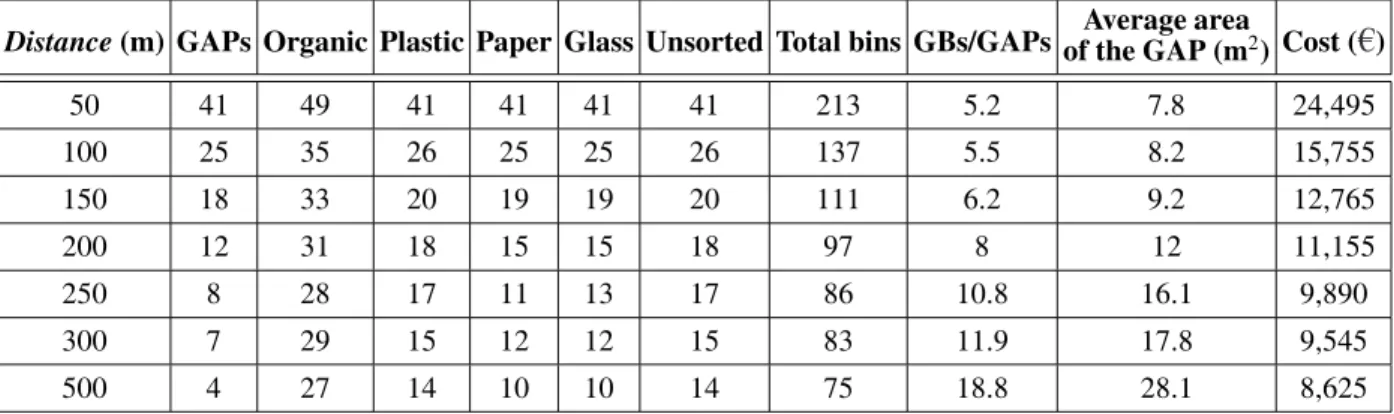
Third campaign of experiments
It was about the execution of theSizingOfGAPs
algorithm for the same seven values of the Dis-tanceparameter. Then, we extracted the results
(Table 9), collected in the SDB, using the fol-lowing SQL query:
SELECT SUM (organic) AS Organic, SUM (plastic) AS Plastic, SUM (paper) AS Paper, SUM (glass) AS Glass,
SUM (unsorted) AS Unsorted, SUM (glass) + SUM (plastic) + SUM (organic) + SUM (paper) + SUM (unsorted) AS "Total bins"
FROM GAP
The 9th column shows that the average number of GBs per GAP increases (from 5.2 GBs to 18.8) as the number of GAPs decreases. The values in the column “Total bins” show, how-ever, that the total number of GBs decreases as the GAPs decrease. This result, apparently sur-prising, can be interpreted by remembering that every GAP consists of at least 5 GBs, one for each category of SW. Since Distance= 50 m gives rise to 41 GAPs, it follows that the min-imum number of GBs is (equal to) 205 (very close to the value 213); whileDistance=500 m gives rise to 4 GAPs, which corresponds to a minimum number of 20 GBs(significantly be-low 75).
The 10th column shows the average value of the area occupied by a GAP, assuming that the area of a single GB is equal to 1.5 m2 (this value is
in line with the size of the GBs available from the network. An example: Pack Services Srl,
http://www.packservices.it).
Lastly, the column “Cost” gives an estimate of the initial investment to be supported. For simplicity, it is assumed that the GBs of dif-ferent types have the same cost(115 , source:
http://www.alibaba.com). It does not escape
the huge difference that exists between the ex-treme cases (Distance = 50 m and Distance = 500 m) due to the 3 to 1 ratio on the to-tal number of GBs. This gap, kept down for the small district of Cansatessa(226 houses and 1,464 residents), becomes relevant if the urban dimension to be served is larger. For instance, in the case of a district hundred times bigger, the initial investment for the two extreme cases is of the order, respectively, of 2.5M and 8.6K . The general finding that can be extracted from the experiments(Table 9)is that the value of the
Distanceparameter should fall between 250 m and 300 m. There are two major reasons sup-porting this choice:
− the resulting number of GAPs and GBs is limited. This implies that the overall waste collection time by the municipal workers is significantly reduced;
− the total number of GBs to be bought is sig-nificantly lower than that in the extreme case
(Distance=50m), which implies a consid-erable economic saving.
From Table 3 and Table 9, we see that the to-tal number of GAPs in Cansatessa is
compara-Distance(m) GAPs Organic Plastic Paper Glass Unsorted Total bins GBs/GAPsof the GAP (mAverage area2) Cost ( )
50 41 49 41 41 41 41 213 5.2 7.8 24,495
100 25 35 26 25 25 26 137 5.5 8.2 15,755
150 18 33 20 19 19 20 111 6.2 9.2 12,765
200 12 31 18 15 15 18 97 8 12 11,155
250 8 28 17 11 13 17 86 10.8 16.1 9,890
300 7 29 15 12 12 15 83 11.9 17.8 9,545
500 4 27 14 10 10 14 75 18.8 28.1 8,625
ble with the outcome produced by our method whenDistance= 300 m(6 vs. 7), but the total number of GBs is definitely insufficient(30 vs. 83). This big mismatch makes evident that the method of allocation adopted nowadays by the municipalities is unsatisfactory. The inevitable consequence is that very often the GBs are full, so it is common to run into scenes like that in Figure 9.
Figure 9.Litter exceeding the storage capacity of the GBs at a GAP.
7. A Nice Feature of the Algorithm
LocatingOfGAPs: the Flexibility
At this point we have all the elements to focus on an interesting behavioral trait of the first al-gorithm. Letgapbe a GAP whose position on
the territory has been identified by LocatingOf-GAPs moving along the public road r. When the algorithm proceeds to explore the roads that are located in the neighborhood of gap(let r*
be one of them), two complementary situations can arise: r* ends before a movement alongr*, starting from gap, equal to Distance has been
accomplished(for brevity we will use the nota-tion: length(gap r*)<=Distance), conversely length(gap r*)>Distance. In the first case, Lo-catingOfGAPsassigns the houses in the residual stretch ofr*(if any)togap; while it manages the
second case with a certain degree of flexibility, as explained below by referring to Figure 10. In Figure 10, the inner area denotes the portion of the urban territory which is far from gapat
most Distance(moving along the public roads of the district), while the crown adds to the in-ternal area a stretch of the public roads equal to
, an arbitrary value much lesser thanDistance. Figure 10 shows, moreover, the three different situations that may arise during the visit of r*
(below renamed r1*, r2*, and r3* to avoid
con-fusing the reader). In the figure, the pointsa,b, andcare distant exactlyDistancefromgapby
moving alongr1*,r2* andr3*.
The following three cases are possible when length(gap r*)>Distance:
1. length(r1*+) <= Distance, i.e., starting
fromgap,r1* ends before a movement equal
toDistance+has been accomplished along such a road. All the houses on r1*, between
pointaand the end ofr1*(two in Figure 10),
are assigned togap;
2. length(r2* + ) > Distance, but beyond
the gray crown there are no other houses to be served, while there are some inside the crown(one in Figure 10). LocatingOfGAPs
assigns those dwellings togap;
3. length(r3*+)>Distance, but beyond the crown there are other houses. In this case
LocatingOfGAPswill ignore any dwellings inside the crown (Figure 10 shows one of them) that will be assigned to a GAP to be positioned when the algorithm visitsr3*.
Figure 10.The light gray centroids denote dwellings assigned togap, while the dark gray ones denote
dwellings not served bygap. The three diamonds
denote the pointsa,b, andc.
The first half of Table 10 repeats results from Ta-ble 9(obtained by setting =25%*Distance), while the second half shows the values that we obtained by eliminating fromLocatingOfGAPs
Table 10, besides confirming what was reason-able to expect (i.e., a systematic increase, for the same value of Distance, of the total num-ber of GAPs and GBs returned by the algorithm
LocatingOfGAPs blindwith respect to Locatin-gOfGAPs), moreover quantifies that the amount of saving we got in the pilot study is mod-est. Notice that it is not possible to predict the amount of saving for given values of Dis-tanceand since it depends on the geography of the district. Obviously, it is up to the recip-ients of our method to carry out a campaign of experiments(for several values ofDistanceand
)in order to identify the best trade-off for the district to be served.
There is a similarity between the “tolerance pa-rameter – ” in (Ghiani et al., 2012) and our
. They set =10%*Distancein the experi-ments.
Table 11 shows fluctuations in the number of GAPs and GBs (for the Cansatessa district)
when varies from 10% to 50% ofDistance.
To not excessively distort the behavior of the algorithmLocatingOfGAPs, it is important that the value ofis kept much lesser thanDistance. For this reason, we suggest do not enter the gray area of Table 11. Doing so, the maximum value of is equal to 20m, 30m, 30m, 40m, 50m, 30m and 50m whenDistancevaries from 50m to 500m, respectively.
The impact of the flexibility of the algorithm
LocatingOfGAPsin exploring the roads in the neighborhood of a GAP is especially important to pursue management of the final stretch of the public roads (a situation which can be traced back to the case of r1* and r2* in Figure 10)
that may be satisfactory from the point of view of the managers of SW collection service. In fact, the shorter the final stretch of the roads, relative to the value of Distance, the less they are inclined towards allocating further GAPs.
LocatingOfGAPs( =25%*Distance) LocatingOfGAPs blind
Distance(m) GAPs GBs GBs/GAP Average area ofthe GAP(m2) GAPs GBs GBs/GAP Average area ofthe GAP(m2)
50 41 213 5.2 9 43 223 5.2 7.8
100 25 137 5.5 9 28 151 5.4 8.1
150 18 111 6.2 10.5 22 130 5.9 8.8
200 12 97 8 12 15 111 7.4 11.1
250 8 86 10.8 16.5 12 104 8.7 13
300 7 83 11.9 18 8 87 10.9 16.3
500 4 75 18.8 28.5 6 82 13.7 20.5
Table 10. A comparison of the results computed byLocatingOfGAPs
andLocatingOfGAPs blindfor the district of Cansatessa.
=10% =20% =30% =40% =50%
Distance(m) GAPs GBs GAPs GBs GAPs GBs GAPs GBs GAPs GBs
50 43 223 43 223 41 213 41 213 40 208
100 27 147 25 137 24 132 24 132 22 128
150 20 121 18 111 18 111 17 107 15 104
200 14 106 13 101 12 99 11 94 11 93
250 9 91 9 91 8 86 8 86 7 83
300 7 83 7 83 7 83 7 82 7 83
500 5 80 4 75 4 75 4 75 4 74
Concluding Remarks
Table 9 tells us that as Distance increases the number of GAPs decreases(as well as the num-ber of the GBs), so it is obvious that the number of GAPs forDistance+ (for any> 0)must be less than that got for Distance. The values in Table 10 confirm this statement. However, it is important to emphasize that the flexibility of the first algorithm cannot be replaced by Lo-catingOfGAPs blindthrough the increase of the parameterDistanceto the valueDistance+. Indeed, there is no increase of able to dis-tinguish the second case in Figure 10 from the third one.
Table 12 compares the results of LocatingOf-GAPswith those ofLocatingOfGAPs blind, the latter run by setting Distance = Distance of
LocatingOf GAPs+ (for example, the values returned by LocatingOfGAPs per Distance =
100m, are compared with those returned by Lo-catingOfGAPs blind run by settingDistance=
125m).
LocatingOfGAPs(=25%) LocatingOfGAPs blind
Distance(m) GAPs GBs Distance(m) GAPs GBs
50 41 213 62.5 37 194
100 25 137 125 24 135
150 18 111 187.5 15 109
200 12 97 250 12 104
250 8 86 312.5 7 81
300 7 83 375 7 81
500 4 75 625 4 73
Table 12.Comparison betweenLocatingOfGAPs
andLocatingOfGAPs blind.
As we can see, the total number of GAPs cal-culated by LocatingOfGAPs blind is less than or equal to the corresponding value calculated byLocatingOfGAPs. We can also note that the deviations decrease as Distance increases, to disappear when Distance >= 300 m. About the GBs, we can see that their total number calculated byLocatingOfGAPs blindis always less than the corresponding value calculated by
LocatingOfGAPs. Also in this case the devia-tions, large for low values of Distance, rapidly decline as Distance increases, and almost dis-appear whenDistance>=300 m.
In summary, it can be said that the reason for the deviations in Table 12 is that while Lo-catingOfGAPstries an action of adjustment of type “local” (according to the schema of Fig-ure 10), that does not always produce savings in the number of GAPs (and, hence, of GBs),
LocatingOfGAPs blind, vice versa, proceeds to the positioning of the GAPs by setting a con-straint about the maximum distance GAP-house less stringent and that produces a saving that is more evident the more we operate at low values ofDistance.
8. Analysis on Demand
As already remarked (Section 4), the strength of the adopted software architecture resides in the technology of the SDBMSs which offers the expressiveness of the SQL language in querying the SDB. The seven queries(consistent with the PostgreSQL/PostGIS syntax)that follow give a concrete proof of the previous statement. Evi-dently, other requirements of analysis that might occur to those who have the responsibility for the management of the SW can be satisfied in the same way.
Q1 Retrieve the total number of the citizens served by each allocated GAP when Distance = 300 m. Order the returned tuples in ascend-ing order of the GAP’s identifier.
SELECT gap id AS "GAP Id", SUM(density) AS "citizens served"
FROM house
GROUP BY gap id
ORDER BY gap id ASC
The output is shown in Table 13.
GAP Id citizens served
1 88
2 205
3 232
4 446
5 144
6 212
7 137
Q2 Retrieve the total number of the houses served by each allocated GAP when Distance = 300 m. Order the returned tuples in ascend-ing order of the GAP’s identifier.
SELECT gap id AS "GAP Id", COUNT (*) AS "houses served"
FROM house
GROUP BY gap id
ORDER BY gap id ASC
The output is shown in Table 14.
GAP Id houses served
1 15
2 37
3 41
4 62
5 24
6 23
7 24
Table 14.The result ofQ2.
Q3Retrieve the identifier of the houses served by each allocated GAP. Order the tuples in as-cending order of GAP’s identifier.
SELECT gap id AS "GAP Id", id AS "house Id"
FROM house
GROUP BY gap id, id
ORDER BY gap id ASC
Output not shown because composed of too many tuples(226).
Q4Retrieve, for each GAP, the value of the av-erage of the distances of the houses served by it. (The SQL formulation refers to Distance =300 m.)
SELECT g.id AS "GAP Id",
round(AVG(distance(h.id, g.id, 400, true))::numeric) AS Distance
FROM gap AS g, house AS h
WHERE St Distance(g.the geom,
h.the geom h)<= 300 AND
distance(h.id, g.id, 400, true) <= 300 AND h.gap id = g.id
GROUP BY g.id
The output is shown in Table 15.
GAP Id AVG distance house – GAP
1 198
2 162
3 85
4 139
5 114
6 150
7 75
Table 15. The result ofQ4.
InQ4,St Distance()is a PostGIS spatial
func-tion, whiledistance()is one of our UDFs. The
first function computes the Euclidean distance between two points(in our case, the position oc-cupied by the GAP and the projection of the cen-troid of the house on the reference road), while the second function computes the distance be-tween the same two points but moving along the public roads. The conditionST Distance(. . .)
<= 300 speeds up the computation of Q4, in fact it asks to ignore all the dwellings that are located more than 300 m as the crow flies, be-cause they will certainly be at a distance not less than 300 m when moving along the roads.
Q5Retrieve the value of the overall average of the distances dwelling-(reference)GAP, when
Distance=300 m.
CREATE VIEW One AS (
SELECT (AVG(distance(h.id, g.id,
400, true))) AS distances
FROM gap AS g, house AS h
WHERE St Distance(g.the geom,
h.the geom h)<= 300 AND
distance(h.id, g.id,
400, true)<= 300 AND
h.gap id = g.id
GROUP BY g.id )
SELECT round((SUM(distances)/COUNT(*)) ::numeric) AS "average distance"
The output is shown in Table 16.
average distance
132
Table 16.The result ofQ5.
The necessity to introduce the viewonecomes
from the impossibility of nesting built-in func-tions(in the example: SUMandAVG)in the
Post-greSQL version we used.
All the previous queries return information in the standard relational format. However, having implemented a SDB, it makes trivial to combine this method of displaying of the results with the construction of maps. Below, we propose two examples, but many others are possible.
Q6Retrieve the location of the dwellings served by GAP 5 andDistance=300 m.
CREATE VIEW Two AS (
SELECT g.id AS "GAP Id", h.id AS house,
h.the geom AS house polygon, h.the geom c AS
house centroid, h.the geom h AS house projection
FROM gap AS g, house AS h
WHERE St distance(g.the geom,
h.the geom h)<= 300 AND distance(h.id, g.id, 400 ::double precision, true) <= 300 AND h.gap id = g.id
GROUP BY g.id, h.id, h.the geom, h.the geom c, h.the geom h
ORDER BY g.id );
SELECT "GAP Id", house polygon
FROM Two
WHERE "GAP Id" = 5;
The output returned byQ6is tabular. Figure 11 shows its visualization through QGIS.
Figure 11. A GIS map built starting from the output ofQ6. The figure shows the twenty-four
dwellings served by GAP 5 and their reference roads(namely: 4, 8 and 11).
Q7 Retrieve the ID and position of the GAPs located along the road “VIA LUDWIG VAN BEETHOVEN”(id=4)andDistance=300 m.
SELECT r.the geom AS road, g.id AS "GAP Id", g.the geom AS Position
FROM road AS r, gap AS g
WHERE r.id = g.road id AND r.name ='VIA LUDWIG VAN BEETHOVEN';
The map in Figure 12 shows that only one GAP
(the small circle) is located along the entered road(id=4).
Figure 12.A QGIS map built starting from the output ofQ7.
the dwellings of the Cansatessa’s district. Q2
provides a global information, while Q3 pro-vides details about the coupling housing-GAP of reference.
Q4 returns, for each GAP, the value of the av-erage distance of the houses it serves, whileQ5
shows the value of the overall average of the distances between each dwelling and its refer-ence GAP. Both those values are of interest to the managers of the service because they pro-vide them with “global” information that enrich the starting data, i.e., the value of the Distance
parameter. The value returned by Q5 (132m) gives the chance to recall the experiments made by Ghiani et al. (2012). They restricted their attention to the values 140 and 150 meters as the maximum distance house-GAP of reference, with the following explanation: those values “are typical distances that can be easily cov-ered in urban areas”. The value 132m rein-forces our belief that the adoption of the con-straintDistance= 300 m might be appropriate in the reality. The added value of the last two queries, compared to the others, is that they also return geometric information, necessary to pro-duce geographic maps invaluable for decision makers.
9. Conclusions and Further Work
Complex decision problems are frequently en-countered in urban planning, typically involv-ing the consideration of a large number of con-flicting objectives. The method proposed in this paper is able to produce a lot of informa-tion to support the persons responsible for the management of the municipal SW in setting, in full autonomy, and in the “real world”, a sat-isfactory trade-off between the maximum dis-tance dwelling-GAP of reference and the num-ber/sizing of the GAPs.
The proposed method was implemented with open source software and then used to carry out a pilot study. The study confirmed what was in a sense obvious to expect, namely that as the dis-tance increases, the number of GAPs decreases. Having few areas of accumulation definitely ac-celerates the waste collection by the municipal workers, while, on the citizens’ side, this may cause some drawbacks. First of all, such a so-lution forces many residents to use the car to go
to drop the SW into the GBs, which may not be the case if the reference GAP is closer(e.g., within 100m). It is also plausible to foresee that such a solution may have impact on the aesthet-ics of the area, on the smells, as well as on the commercial value of the surrounding dwellings. Another aspect not to be underestimated is the fact that it may not be trivial to find, within mod-ern urban areas, sites adequate to accommodate large GAPs. Last, but not least, decision makers may be constrained in the choice of a solution by the budget available. Our study pointed out clearly that the initial investment to buy the GBs decreases as the value ofDistanceincreases. In closing, it is worthwhile to repeat that the es-timate of the number of GBs within each GAP is directly related to the availability of certain data about the number of people living inside the dwellings and the daily production of waste by each dwelling. It serves, also, to know what is the conversion factor of the weight of the SW
(expressed in kg) in space (m3), because this latter value has to be correlated with the capac-ity of the bins(expressed in m3). Obviously, the responsibility to get hold of this input data is a burden to the society, either private or public, responsible of the management of the SW.
Further Work
The solution described in this article can be ben-efited by the end users with a training on the job of a few hours. In fact, to make the elaborations about the location and the sizing of the GAPs for varying values of the Distance parameter, it is sufficient to invoke, from inside the Post-greSQL query window, the command:
SELECT solveSWAP(distance);
where solveSWAP() is the UDF collecting the
PL/pgSQL code that implements our two algo-rithms. Similarly, the processing of the queries listed previously can be invoked by copying their SQL code in the same window.
makers can access the services available to them in conditions of total independence from the ar-chitectural/technological underlying elements.
References
[1] M. F. BADRAN, S. M. EL-HAGGAR, Optimization of municipal solid waste management in Port Said – Egypt.Waste Management26, 534–545, 2006.
[2] J. BAUTISTA, J. PEREIRA, Modeling the problem of
locating collection areas for urban waste manage-ment, an application to the metropolitan area of Barcelona. Omega. The International Journal of Management Science34, 617–629, 2006.
[3] A. M. DAMGHANI, G. SAVARYPOUR, E. ZAND, R.
DEIHIMFARD, Municipal solid waste management
in Tehran: Current practices, opportunities and challenges.Waste Management28, 929–934, 2008.
[4] P. DIFELICE, Integration of spatial and descriptive
information to solve the urban waste accumulation problem. 3rd Inter. Conf. on Integrated Informa-tion (IC-ININFO), Prague, Czech Republic, Sept. 5–9, 2013. Elsevier, Procedia – Social and Behav-ioral Sciences pp. 182–188, 2014. DOI information: 10.1016/j.sbspro.2014.07.150.
[5] EEA, Managing municipal solid waste. A re-view of achievements in 32 European countries.
Report by the European Environment Agency.
http://www.eea.europa.eu/publications/m naging-municipal-solid-waste(Retrieved on
June, 2013).
[6] R. FELIX, J. GARCIA-VEGA, Quality of Life in
Mexico: A Formative Measurement Approach. Ap-plied Research Quality Life,7:223–238, 2012. DOI 10.1007/s11482-011-9164-4.
[7] G. GHIANI, D. LAGANA`, E. MANNI, C. TRIKI,
Ca-pacitated location of collection sites in an urban waste management system.Waste Management,32, 1291–1296, 2012.
[8] D. HOORNWEG, P. BHADA-TATA, What a waste:
A Global Review of Solid Waste Management. Urban Development & Local Government Unit, World Bank, Washington, DC 20433 USA, 2012.
www.worldbank.org/urban
[9] S. LEBERSORGER, P. BEIGL, Municipal solid waste generation in municipalities: Quantifying impacts of household structure, commercial waste and do-mestic fuel. Waste Management, 31, 1907–1915, 2011.
[10] M. MIYAZAKI, T. IMATOH, H. UNE, The treatment of infectious waste arising from home health and medical care services: Present situation in Japan.
Waste Management,27, 130–134, 2007.
[11] OBRA, Official Bulletin of Regione Abruzzo – Speciale Ambiente n.25, 15 April 2011 –
http://bura.regione.abruzzo.it/2011/Spe ciale 25 15 04.pdf(Retrieved on June 2013).
[12] L. PARROT, J. SOTAMENOU, B. K. DIA, Municipal
solid waste management in Africa: Strategies and livelihoods in Yaound´e, Cameroon.Waste Manage-ment,29, 986–995, 2009.
[13] C. S. REVELLE, H. A. EISELT, Location analysis: a
synthesis and survey.European Journal of Opera-tional Research,165, 1–19, 2005.
[14] G. TCHOBANOGLOUS, H. THEISEN, S. VIGIL,
In-tegrated Solid Waste Management. McGraw-Hill, New York, 2005.
[15] L. TRALHAO˜ , J COUTINHO-RODRIGUES, L. ALCADA¸
-ALMEIDA, A multiobjective modeling approach
to locate multi-compartment containers for urban-sorted waste.Waste Management,30, 2418–2429, 2010.
[16] UN-HABITAT, Solid waste management in the world’s cities.United Nations Human Settlements Programme, 2010.
[17] US EPA.(2010). Municipal Solid Waste Genera-tion, Recycling, and Disposal in the United States. United States Environmental Protection Agency.
http://www.epa.gov/osw/nonhaz/municipal /pubs/msw 2010 factsheet.pdf.
EPA-530-F-11-005, November 2011.(Retrieved on June 2013).
[18] H. ZIA, V. DEVADAS, Urban solid waste
manage-ment in Kanpur: Opportunities and perspectives.
Habitat International,32, 58–73, 2008.
Received:May, 2014
Revised:October, 2014
Accepted:December, 2014
Contact address:
Paolino Di Felice Department of Industrial and Information Engineering & Economics University of L’Aquila L’Aquila Italy e-mail:[email protected]
PAOLINODIFELICEis Professor of Computer Science at the Department of Industrial and Information Engineering & Economics of the Univer-sity of L’Aquila. He has authored or co-authored about 100 articles in international journals, books, and conference proceedings in the areas of programming methodologies, relational and spatial databases. He has also carried out a consistent activity of technological transfer in collaboration with several IT firms. His research has been funded by national and international institutions and carried out in collaboration with researchers of several countries(Italy, Holland, Germany, Canada, and the USA). He has served within national and international com-mittees. In the last years, he is permanently member of the program committee of the International Conference on Integrated Information