Vol. 12, No. 4, 2019, 1612-1642 ISSN 1307-5543 – www.ejpam.com Published by New York Business Global
Density and Risk Function of Circular Kernel Study
Didier Alain Njamen Njomen1,∗, Hubert Clovis Yayebga1
1 Department of Mathematics and Computer’s Science, Faculty of Science, University of Maroua, Maroua, Cameroon
Abstract. In this article, based on the works of [18], [22] and [26] on the estimation of the survival function and the function of risk in independent cases and identically distributed with and without censorship, We manage to established the bias and variance of the density of the circular kernel. In addition, we determined the optimal windowb∗n of this estimator after having first established the mean square error (MSE) and mean integrated squared error (MISE) which are necessary conditions for obtaining the optimal window. Finally, we have established the asymptotic expression of the bias of the risk function of the circular kernel estimator.
2010 Mathematics Subject Classifications: 97K80, 62G07, 11R45
Key Words and Phrases: Nonparametric estimator, Density function, Risk function, Circular kernel, Bias, Mean squared error, Mean integrated squared error, Optimal window
1. Introduction
Survival analysis refers to a set of statistical techniques for processing censored data which is unknown for some of them, that a lower or higher bound and not a precise value. It represents the study of the delay of the occurrence of an event. It is called survival anal-ysis or lifetime data analanal-ysis which is present in several areas of life among which we can mention the medicine to evaluate the effectiveness of a treatment. In demography to build life tables where these are used by actuaries to determine the amount of life insurance and life annuities, among others; actuarial tables are used when data is grouped into intervals. It is also in engineering to estimate the reliability of machines and electronic components. Survival analysis is also useful in astrophysics. Imagine that sources have been detected at a wavelengthλand that we observe at the same positions another wavelengthλ0. Some sources are not detected at λ0 because the ratio signal/noise (l0/b) is too low. However, how to calculate the color distribution m−m0 = 2,5 log10(l0/l) +constant? hence the interest in physics survival analysis. This analysis is linked to an event that is the subject of a study and that is how we will be able to study its lifespan or survival.
∗
Corresponding author.
DOI: https://doi.org/10.29020/nybg.ejpam.v12i4.3519
Email addresses: [email protected](D. A. N. Njamen),[email protected](H. C. Yayabga)
The term survival time refers to the time elapsed until the occurrence of a specific event. The event studied (commonly called death) is the irreversible transition between two states (commonly called living and death). The terminal event is not necessarily death: it can be the appearance of a disease (for example, the time before a relapse or rejection of a transplant), a cure (time between the diagnosis and the cure), the breakdown of a machine (duration of operation of a machine, in reliability) or the occurrence of a disaster (time between two disasters, in actuarial).
In survival analysis, the estimation of the hazard function is an interesting problem that appears in the statistical analysis of useful life to study several types of events.
Many methods have been proposed to study the estimation survival functions and risk functions in independent and identically distributed (i.i.d) cases with and without censor-ship. We can mention among others: [19], [17], [9], [18], [22], [20], [3], [21], [26], [8], [23], and [16]. However, the study of the determination of the mean squared error (MSE) and the mean integrated squared error (MISE) to obtain the optimum window of the circular kernel remains unclear. This article brings a relief to this problematic.
This article is subdivided into six parts: The first part is devoted to the development of the different notions studied in the density and risk functions. The second part deals with the estimation of kernel density function. The third part deals with the risk function estimation. The fourth part reminds us of the notion of mean squared error (MSE). In the fifth part, it’s about the probability and risk function of the circular kernel. Finally in the last part, through simulated and real data, we show that our estimator is efficient.
2. General results on density and risk functions
In this section, we acquire various basic concepts that allow a good understanding of our work. For this purpose, we have been inspired by the founding works, articles and even courses read online. This among others include the works by: [1], [22], [3], [5] and [23]. The survival time T refers to the time elapsed since an initial moment (beginning of treatment, diagnosis, unemployment, ...) until the occurrence of an event of final interest (death of the patient, relapse, remission, healing, work, ...). It is said that the individual survives the time t if at this moment the event of final interest has not yet taken place. The variable studied is called survival time and will be marked T.
2.1. Expression of the density and risk functions in survival analysis
Let T be the survival time that is assumed to be a positive variable. Its probability law can be defined by one of the following functions:
2.1.1. Probability density function
Definition 1. The probability density function of T, denoted f(t) is defined by:
f(t) = lim
∆t→0+P
t≤T ≤t+ ∆t ∆t
. (1)
For fixed t, the probability density is interpreted as the probability that the event occurs in the short time interval ]t, t+ ∆[.
2.1.2. Risk function
Definition 2. The risk function of T denotedh(t) is defined by:
h(t) = (
lim∆t→0 P(t<T
≤t+∆t|T >t)
∆t , if t >0 and such thatP(T > t)>0;
+∞ if not. (2)
For fixed t, the risk function h is the instantaneous risk that the event occurs in the interval ]t, t+ ∆[ knowing that it did not take place before time t (being in ”operation” or be ”alive” before timet).
Remark 1. The risk function is also called hazard function, chance rate, failure rate or survival rate.
The risk function may have different forms but is necessarily positive on R.
Suppose now that T is a continuous variable, we observe that the risk function is defined by:
h(t) = lim
∆t→0
P(t < T ≤t+ ∆t|T > t)
∆t
= lim
∆t→0
1 ∆t
P(t < T ≤t+ ∆t)
P(T > t) =
f(t)
S(t), (3)
whereS =P(T > t) is the survival function.
The Hazard function characterizes the law of T because of the relation: S(t) = exp(−
Z t
0
h(u)du).
2.1.3. Cumulative risk function
Definition 3. The cumulative risk function Λ(t) is defined by:
Λ(t) = Z t
0
2.2. Different forms of the risk function
In this subsection we give the main forms of law used in survival data. The usual forms of the functionh are constant, monotonous (increasing or decreasing) and in the form of
∩.
2.2.1. Constant risk
The only distribution that has a constanth risk function is the exponential law.
The probability density and the risk functionhare respectively defined by the exponential law denotedε(λ):
f(t, λ) = λe−(λt), t≥0; h(t) = λ.
2.2.2. Monotonous risk
There are several life-time distributions with a monotonic risk function.
• Weibull LawW(λ, α)
There are several life-time distributions with a monotonic risk function. f(t, α, λ) = αλαtα−1e−(λt)α;
h(t) = αλαtα−1.
The parameter α is a form parameter ofh and λis a scale parameter. Remark 2. (i) If α= 1, we obtain the exponential law W(λ,1) =ε(λ)
(ii) If 0< α <1, the risk functionh is decreasing from ∞ to 0
(iii) If α >1, the risk functionh is increasing from (0 to ∞).
• Gamma Law Γ(λ, β)
The probability density and the risk function are respectively defined by the Gamma law:
f(t, λ, β) =λβ 1 Γ(β)t
β−1e−λt, λ, β >0, t≥0;
h(t, λ, β) = f(t, λ, β) 1−F(t, λ, β).
The parameter β is the form parameter of h andλis scale parameter.
Remark 3. (i) Ifβ = 1, we obtain the exponential law with parameterλ: Γ(λ,1) = ε(λ)
2.2.3. Risk in ∩
• Log-normal lawLN(λ, v)
The probability density and the risk function are respectively defined by the Log-Normal lawLN(µ, σ):
f(t, µ, σ) = 1 σtϕ
lnt−µ σ
;
h(t, µ, σ) = f(t, µ, σ) S(t, µ, σ).
Remark 4. The risk functionhis in the form∩: it increases from 0 to its maximum value and then decreases to 0.
• Log-logistic Law LL(λ, v)
The probability density and the risk function are defined respectively by the log-logistic law:
f(t, λ, v) = (λv)λtv−1(1 + (λt)v)−2; h(t, λ, v) = (λv)λtv−1(1 + (λt)v)−1.
Remark 5. Thev parameter is a form parameter ofh. Forv >1, the risk function
h increases from 0 to its maximum value and then decreases to 0.
3. Density function estimation
3.1. Kernel estimator: case of uncensored data
The concepts used in this section come from the following documents: [19], [17], [11], [24], [9], [20], [3], [20] and [23].
LetT1, T2, ..., Tndistribution function survival durationsFand letVx0 =]t0−b2n, t0+b2n[
a neighborhood oft0, where (bn)n≥0 is a sequence of positive parameters called window.
An estimator of the density f at the point t0 is given by:
fn(t0) =
Fn(t0+b2n)−Fn(t0−b2n) bn
= number of events on ]t0−
bn
2 , t0+ bn
2 [ bn
,
whereFn is the empirical distribution function.
We can also write it in the following form:
fn(t0) =
1 nbn
n
X
i=1
11]t0−bn
2 ,t0+
bn
2 [
= 1 nbn
n
X
i=1
11]−1 2,
1 2]
t0−Ti bn
.
This writing shows a function K called kernel, which is in the form: K(.) = 11]−1
2, 1 2](.).
Hence the definition of a kernel estimator of f, fort∈
−1 2,
1 2
:
b
fn(t) =
1 nbn
n
X
i=1 K
t−Ti bn
, (5)
where the kernel K is an application of R on R+, bounded, of integral equal to 1,
sym-metrical and of morebn→0 whenn→+∞.
3.1.1. Examples of kernels
The various kernels most used in estimating the density are:
• Gaussian kernel
∀u∈R, K(u) = √1
2πe
−u2
2 (6)
• Uniform kernel
∀u∈R, K(u) = 1
211|u|≤1 (7)
• Epanechnikov kernel
∀u∈R, K(u) = 3 4(1−u
2)11
|u|≤1 (8)
• Triangular kernel
∀u∈R, K(u) = (1− |u|)11|u|≤1 (9)
• Quadratic kernel
∀u∈R, K(u) = 15 16(1−u
2)211
|u|≤1 (10)
Definition 4. A kernelKis called Parzen-Rosemblatt ifK is symmetric and iflim|u|→∞|u|K(u) = 0.
If we considerKbn(y) =
1 bnK(
y
bn), kernel estimatorfn is written:
fn(t) =
Z +∞ −∞
3.1.2. Optimal choices of kernel K and window bn
The convergence results of the kernel estimatorfn require conditions on K and bn, from
which the problem of the optimal choice of (K, bn).
We pose:
∆n(t) = E[fn(t)−f(t)]2
= E[fn(t)−Efn(t) +Efn(t)−f(t)]2
= [Efn(t)−f(t)]2+E[fn(t)−Efn(t)]2.
It is assumed that the kernel supportK is [−1,1].
The following theorem gives the asymptotic behavior of the bias and the variance of the estimatorfn.
Theorem 1. ([3])
If f is of class C2 and K is a kernel of Parzen-Rosemblatt. So if bn→ 0 and nbn→ ∞, we have:
•
Bias(fn(x)) = b2n
2 f 00
(x) Z
R
t2K(t)dt+O(b2n). (11)
•
Var(fn(x)) =
1 nbn
f(x) Z
R
K2(t)dt+O
1 nbn
. (12)
The choice of the optimal window b∗n is done if the kernelK is given. The smoothing parameterbn is a positive real whose choice is preponderant over that of the symmetrical
continuous kernelK. Choosing a value of bn too big leads to a curve that is too smooth.
On the other hand, by choosing a very small smoothing parameter than the one previously adopted, the shape of the distribution changes.
Theorem 2. ([3])
Under the conditions of the theorem 1, the optimal window is:
b∗n= f(t) f002(t)R
u2K(u)du2 Z 1
−1
K2(u)du
!1
5
n−15. (13)
3.2. Kernel estimator: case of censored data
The purpose of this subsection is to estimate the density of survival times T in the context of censored data.
LetT1, T2, ..., Tnbe a sequence of positive random variables i.i.d of distribution function
F representing survival times and C1, C2, ..., Cn is the sequence of random variables i.i.d
representing censoring, of distribution function G. We assume that the sequence (Ti) is
Kaplan-Meier estimator [6] of the survival function S is given by:
b
SKM(t) =
Y
t(i)≤t
1− 1
n−i+ 1 D(i)
. (14)
It can also be written in the form:
b
SKM(t) =
( Q
X(i)≤t
1− D(i) n−i+1
si t≤X(n)
1−Fbn(X(n)) t > X(n), where X(1)<X(2)<...<X
(n) is the order statistic of the sample X1, X2, ..., Xn and D(i) is the
value of Di (the right censorship flag) associated with X(i).
Fort > X(n)we considered 1−Fbn(t) = 1−Fbn(X(n)) since there is no more observations after t. This estimator (SbKM(t)) of survival function was studied by [13], [14], [15] in the context of competing risks.
We assume that F admits a density f in relation to Lebesgue’s measure proposes to estimate using the observations (Xi, Di), I = 1, ..., n. Based on the Kaplan-Meier
estimator, [2] proposed an estimator of the density f by the kernel method given by: fn(t) =
1 bn
Z +∞
0 K
t−s bn
dFbn(s), (15)
where Fbn is an empirical distribution function, (bn)n≥1 is the window with bn → 0 when
n→ ∞ and K a kernel of support [−1,1].
This estimator fn has been studied in particular by [2], [4] and [10].
4. Risk function estimation
4.1. Kernel estimator: case of uncensored data
In this part, we will study an estimator of the risk function in the case of uncensored data, by the method of kernel by developing the article written by [18].
In 1983, Henrik Ramlau-Hansen had proposed a methodology, cited by [7], to con-struct an estimatorbhnof the risk function by smoothing. This smoothing occurs through convolution by a kernel and by use of a windowbn.
Let T1, T2, ..., Tn the random variables i.i.d of density f and F distribution function.
The kernel estimator of the density proposed by [19] is defined by:
b
fn(t) =
1 bn
Z +∞ −∞
K
t−s bn
dFn(s), (16)
whereFn is the empirical distribution function ofTi andK a Parzen-Rosenblatt kernel of
on Rand lim|x|→+∞|x||K(x)|= 0). Recall that the risk function
h(t) = f(t)
1−F(t), (17)
witht≥0 andF(t)<1.
[25] studied a kernel estimator of risk functionh given by:
b
hn(t) =
1 n−i+ 1
n
X
i=1
1 bn
K
t−Ti bn
, (18)
whereT(1), T(2), ..., T(n) is the order statistic ofTi.
If we pose
Nn(t) =nFn(t) = n
X
i=1
11{Ti≤t} and
Yn(t) =n−Nn(t)(t−) = n
X
i=1
11{Ti≥t}, then, the expression (18) can be written in the form:
b
hn(t) =
1 bn
Z +∞
0 K
t−s bn
dHbN A(s), (19)
where
b
HN A(t) =
Z t
0
dNn(s) Yn(s)
(20) is the Nelson-Aalen estimator of the cumulative hazard rate (see [12], [1] and [13]). Definition 5. Let K be a bounded function of integral 1 and bn a positive window. The kernel estimator corresponding to the h hazard rate is given by:
bhn(t) = 1 bn
Z 1
0 K
t−s bn
dHbN A(s). (21)
The instants of process N jumps are T(1), T(2), ..., T(n). So,
b
hn(t) = 1 bn
P
iK( t−T(i)
bn )
Yn(T(i))
4.2. Mean and variance of the kernel estimator bhn
We assumed that the support of the kernel K is [−1,1] and 0 < bn< 12. Let consider t∈[bn,1−bn]. Then we have:
ehn(t) = 1 bn
Z 1
0 K
t−s bn
dHen(s) = Z 1
−1
K(u)h(t−bnu)J(t−bnu)du,
withJ(t) = 11{Y(t)>0}. Proposition 1. ([8]) By taking,
Kbn(s) = 1 bn
K
s bn
and
jn(s) =E(Jn(s)) then for all t≥0, we have:
E(bhn(t)) =E(ehn(t)) = (Kbn∗hjn)(t), (23)
and,
σn2(t) =E
bhn(t)−ehn(t) 2
= 1 bn
Z 1
−1
K2(u)h(t−bnu)E
Jn(t−bnu) Yn(t−bnu)
du, (24)
with jn(t)) = 11{Yn(t)>0}.
Proposition 2. ( [8])
For all t∈[bn,1−bn], an unbiased estimator of σ2 is
b
σ2(t) = 1 b2 n
Z 1
−1
K2(t−s bn
) Jn(s) Y2n(s)
!
dNn(s), (25)
with jn(t)) = 11{Yn(t)>0}.
4.3. Kernel estimation of the risk function: case of censored data
In this subsection, we drew on the work of [22].
Let the survival durations T1, T2, ..., Tn of distribution function F and densityf and C1, C2, ..., Cn the censorship random variables and FC their distribution function. It is
assumed thatTi are independent ofCi for alli= 1, ..., nand we observeXi=Ti∧Ci and Di= 11{Ti≤Ci}. We denotefX the density ofXi and FX their distribution function. Recall that the kernel estimator of the risk function ofTn is given by:
b
hn(t) = n
X
j=1
D(j)
n−j+ 1Kbn(t−X(j)) =
n
X
i=1
D(i) n−Ri+ 1
whereX(1), X(2), ..., X(n) is the statistic of order and Ri the rank of Xi.
This estimator appeared for the first time in the work of [25] and developed [18]. For the rest, we assume that:
(i) The risk function h is continuous and 0< F(y)<1.
(ii) The kernel K is symmetric, positive and K(t) = O(t−1) when t → +∞ and R
K(t)dt= 1.
4.4. Mean and variance of the estimator bhn
Let
m(y) = f(y) [1−FC(y)] fX(y)
withfX(y)>0.
To determine the mean and the variance ofbhn, we need the following lemma: Lemma 1. ([22])
For all j, we have:
E(D(j)/X(j)=y) =m(y), (27)
and for all r < s, y < z, we have:
E(D(r)D(s)/X(r) =y, X(s)=z) =m(y)m(z). (28)
The following theorem gives the mean and the variance ofbhn. Theorem 3. ([22])
We have:
E
b
hn(t)
=
Z
(1−FXn(y))h(y)Kbn(t−y)dy, (29)
and,
V
b
hn(t)
=
Z
In(FX(y))h(y)Kb2n(t−y)dy+ 2 Z Z
y≤z
{FXn(z)−FXn(y)FXn(z) (30)
− 1−FX(y)
FX(z)−FX(y)
[FXn(z)−FXn(y)]}h(y)h(z)Kbn(t−y)Kbn(t−z)dydz,(31)
where
In(FX) = n
X
k=0
5. Mean Squared Error
In statistics, the mean squared error (MSE) of an estimator θbwith a parameter θ of dimension 1 is a measure characterizing the precision of this estimator. It is more often called quadratic risk.
Definition 6. The mean squared error is defined by:
M SE(bθ) =E h
(bθ−θ)2 i
. (32)
Mean squared error can be expressed as a function of bias and the variance of the estimator hence the following theorem:
Theorem 4. ([5])
M SE(θb) =Biais(θb)2+V ar(θb). (33) Remark 6. As the name suggests, the mean integrated squared error (MISE) is in fact the integration made on the mean squared error.
6. Probability Density and Risk Function of the Circular Kernel
In this section, we consider a sequence (xi)ni=1 of random variables according to an
un-known probability densityf and such thatfhas a continuous second derivative. Moreover, we work within the strict case of non censored data.
6.1. Circular Kernel
The circular kernel still called the cosine kernel is defined by: K(t) = π
4 cos π
2t
.11{|u|≤1}. (34)
The expectation and variance of the circular kernel, were defined by [3].
Proposition 3. Let X be a random variable following a circular law then its expectation and its variance are given by:
• E(X) = 0
• V(X) = 1−π82.
6.2. Circular kernel estimator
The density estimator probability f associated to a circular kernel is given by:
b
f(x) = 1 nbn
n
X
i=1 K
xi−x bn
= 1
nbn n
X
i=1 π 4 cos
π 2(
x−xi bn
)
6.3. Risk function estimation of the circular kernel estimator
In this section, we are talking about estimating the risk function of the circular kernel. Definition 7. The kernel estimator of the hazard function is defined by:
b
h(x) = fb(x) 1−Fb(x)
= fb(x) b
S(x),
whereF(.) andS(.) respectively designate the distribution and survival functions;Fb(.) and Sb(.) their respective estimators.
7. Main results
7.1. Case of the circular kernel estimator
7.1.1. Bias and Variance of the circular kernel estimator
The bias and variance of the circular kernel estimator is given by the following proposition and is the first result of this article.
Proposition 4. The bias and variance of the circular kernel estimatorfbof the relation
(35) is given respectively by:
E
b
f(x)−f(x) = b
2 n
2f 00(x)
1− 8
π2
+O(b2n). (36) (37)
and
V(fb(x)) = 1 nbn
f(t)π
2
16 +O
1 nbn
. (38)
Proof. LetX1, X2, ..., Xn be random variables that are i.i.d. We then have:
•
E(fb(x)) = E ( 1 n n X i=1 1 bn K
x−Xi bn ) = 1 n n X i=1 E 1 bn K
x−Xi bn = E 1 bn K
x−X1 bn = Z R 1 bn K
x−x1 bn
f(x1)dx1
Hence,x1 =bnt+x.
From the expression of x1 above, we obtain:
E(fb(x)) = Z
R
K(−t)f(x+bnt)dt.
Thus,
Bias(fb(x)) = E(fb(x)−f(x)) =
Z
R
K(−t)f(x+bnt)dt−f(x)
= Z
R
K(t)f(x+bnt)dt−f(x) because K is symmetrical.
In an aim to obtain a simpler form, which depends only on the parameter bn, we
approximate the bias formula using the Taylor-Lagrange formula: f(x+bnt) =f(x) +bntf0(x) +
b2nt2 2 f
00(x) +O(b2 nt2).
Thus, replacing the expression off(x+bnt) in the expression of Bias(fb(x)) above, we get:
Bias(fb(x)) = Z
R
K(t)
f(x) +bntf0(x) + b2nt2
2 f
00(x) +O(b2 nt2)
dt−f(x) = f(x)
Z
R
K(t)dt+bnf0(x)
Z
R
tK(t)dt
+ 1
2b
2 nf
00 (x)
Z
R
t2K(t)dt−f(x) +O(b2n).
And according to our assumptions on the K kernel, we finally get: Bias(fb(x)) =
b2n 2 f
00 (x)
Z
R
t2K(t)dt+O(b2n), so,
Efb(x)−f(x) =
b2n 2 f
00(x) Z
R
t2K(t)dt+O(b2n). Yet,
Z
R
t2K(t)dt= Z 1
−1
t2K(t)dt= 1− 8
π2,
so, by replacing it in our expression above, we obtain:
E
b
f(x)−f(x) = b 2 n 2f 00
(x)
1− 8
π2
Hence,
Bias(fb(x)) =E
b
f(x)−f(x) = b 2 n 2 f 00
(x)
1− 8
π2
+O(b2n). Hence the bias offb.
• Starting from the assumption of independence between theXi, we have:
Var(fb(x)) = Var ( 1 n n X i=1 1 bn K
x−Xi bn
)
= 1
nV ar
1 bn
K
x−X1 bn = 1 nE " 1 bn K
x−X1 bn 2# − 1 n E 1 bn K
x−X1 bn 2 = 1 n Z R 1 h2K
2
x−x1 bn
f(x1)dx1−
1 n Z R 1 bn K
x−x1 bn
f(x1)
2
.
By performing the −t= x−bx1
n variable change, we get:
V(fb(x)) = 1 nb2
n
Z
R
K(−t)2f(x+bnt)bndt−
1 n
Z
R
K(−t)f(x+bnt)bndt
2
= 1
nbn
Z
R
K(t)2f(bnt+x)dt−
1 n
h
Biais(fb(x)) +f(x) i2
= 1
nbn
Z
R
K(t)2f(bnt+x)dt−
1 n
O(b2n) +f(x) 2
= 1
nbn
Z
R
K2(t)
f(x) +bntf0(x) + bn
2 t
2f00(x) +O(b2 nt2)
− 1
n
O(b2n) +f(x) 2
= 1
nbn f(x)
Z
R
K2(t)dt+ 1 nf
0 (x)
Z
R
tK2(t)dt+ 1 nbnf
00 (x)
Z
R
t2K2(t)dt
− 1
n
O(b2n) +f(x) 2.
Yet,
Z
R
tK2(t)dt= Z 1
−1 tπ
4 cos( π 2t)
2
(t)dt= 0, We have:
V(fb(x)) = 1 nbn
f(x) Z
R
K2(t)dt+ 1 nbnf
00(x)Z
R
t2K2(t)dt− 1
n
Finally, under the condition of having RK(t)2dt <+∞ and forn large enough, we have:
V
b
f(x)
= 1 nbn
f(x) Z
R
K(t)2dt. By elsewhere,
Z
R
K2(t)dt= Z 1
−1
K2(t)dt= Z 1
−1 π2 16cos
2(π
2t)dt= π2 16, Hence the variance of fbis:
V(fb(x)) = 1 nbn
f(x)π
2
16 +O
1 nbn
.
To determine the optimal window, we first need to find the MSE and the MISE of the estimator fb. In statistics, the mean squared error is a way of estimating the difference between an estimator and the actual value of the quantity to be calculated. It provides a way to choose the best estimator. The proposition gives the mean squared error (MSE) and the integrated mean squared error (MISE) of the circular kernel estimator, and is therefore the second result of this paper.
7.1.2. Mean squared error (MSE) and mean integrated squared error (MISE) The mean squared error (MSE) and the mean integrated squared error (MISE) of the circular kernel estimator are given by the following result:
Proposition 5. The Mean Square Error (MSE) and the Mean Integrated Squared Error (MISE) of the circular kernel estimator fbof the relation (35) are given respectively by:
(i) M SE(fb)≈ b
4
n
4 (1− 8 π2)2f
002(x) + π2 16nbnf(x);
(ii) M ISE(fb)≈
b2
n
4(1− 8
π2)2I1+ π 2 16nbnI2,
where I1 =
R
f002(x)dxand I2 =
R
f(x)dx. Proof.
(i) According to the definition of the mean squared error, we have:
M SE(fb) = V(f(x)) +Bias(fb(x))2
= 1
nbn f(x)π
2
16 +O( 1 nbn
) +
b2n 2 f
00(x)
1− 8
π2
+O(b2n) 2
≈ 1
nbn f(x)π
2 16 + b2 n 2 f 00(x)
1− 8
π2
≈ b
4 n
4 (1− 8 π2)
2f002(x) + π2
16nbn f(x). So, theM SE(fb).
(ii) We know thatM ISE(fb) = R
M SE(fb)dx, then we have:
M ISE(fb) = Z
M SE(fb)dx
≈
Z
b4n 4 (1−
8 π2)
2f002(x) + π2
16nbn f(x)
dx
≈ b
4 n
4 (1− 8 π2)
2
Z
f002(x)dx+ π
2
16nbn
Z
f(x)dx.
By posingI1 =
R
f002(x)dxand I2 =
R
f(x)dx, we obtain: M ISE(fb)≈
b4 n
4 (1− 8 π2)
2I 1+
π2
16nbn I2.
7.1.3. Optimal window of the circular kernel estimator
The following result gives the optimal window of the estimator (35) and is the third result of this article:
Theorem 5. The optimal window of the kernel estimator fbof the relation (35) is given
by:
b∗n=π 5
s
πI2
16nI1(π2−8)2
. (39)
Proof. To determine the optimal window, we look for the value of the window which minimizes the integrated mean squared error.
For that, let’s look for the value ofbnthat minimizes the integrated mean squared error.
According to the above proposal, we have: M ISE(fb)≈
b4n 4(1−
8 π2)
2I 1+
π2 16nbn
I2.
By deriving M ISE(fb), we have:
∂ ∂bn
M ISE(fb) =
∂ ∂bn
b4 n
4(1− 8 π2)
2I 1+
π2
16nbn I2
= b3n
1− 8
π2
2
I1− π2 16nb2
n I2.
By canceling the derivative above, we have: ∂
∂bn
M ISE(fb) = 0 ⇔ b3n
1− 8
π2
2
I1− π2 16nb2
n I2 = 0
⇔ b5n
1− 8
π2
2
I1 = π2 16nI2
⇔ b5n=
π2 16nI2
1−π82
2
I1
⇔ bn= 5
v u u t
π2 16nI2
1−π82
2 I1 . Moreover, ∂2 ∂b2 n
M ISE(fb) = 3b2n
1− 8
π2
2
I1+ π2 8nb3
n
I2 >0.
As the quantities 3b2n 1− 8 π2
2
and 8nb3nare positive, and sinceI1 andI2 are also positive
according to condition (C.4), then we conclude that the value of bn that minimizes the
integrated mean squared error is:
b∗n=π 5
s
πI2
16nI1(π2−8)2 .
Hence the result.
7.1.4. Optimal mean integrated squared error (M ISEopt)
The following result gives the optimal integrated mean squared error (M ISEopt) of the
estimator (35) and represents the 4th result of this article.
Theorem 6. The optimal mean integrated squared error denoted (M ISEopt) of the esti-mator (35) is given by:
M ISEopt(fb) = 5
π4I1I24(π2−8)2
413×n4
15
. (40)
Proof.
We know that the optimal mean integrated squared error(M ISEopt) of the estimator
(35) can be written in the form: M ISEopt(fb) =
b∗n4 4 (1−
8 π2)
2I 1+
π2 16nb∗
Then, by replacing the optimal window b∗n by its value, we obtain: M ISEopt(fb) =
b∗n4 4 (1−
8 π2)
2I 1+
π2 16nb∗nI2
= π
4
4
1− 8
π2 2 I1 5 s πI2
16n(π2−8)2
4 + π 2I 2 16nπ 5 s
16nI1(π2−8)2 πI2
= 1
4
(π2−8)2π45I 4 5 2I 1 5 1
(16n)45(π2−8) 8 5 + π 16n I 4 5 2I 1 5 1(16n)
1
5(π2−8) 2 5
π15
= 1
4
(π2−8)25π45I45 2I
1 5 1
(16n)45
+π 4 5I 4 5 2I 1 5
1(π2−8) 2 5
(16n)45
= 5
4 π45I
4 5 2I
1 5
1(π2−8) 2 5
(16n)45
= 5
π4I1I24(π2−8)2
413×n4
15
.
Hence the result.
7.2. Case of the risk function
The following theorem gives the bias and variance of the circular kernel risk function estimator and is the 5th result of this article.
Theorem 7. The bias and variance of the risk function estimatorbh of the circular kernel
are respectively given by:
Biais(bh(x)) =
b2nf00(x)(π2−8)
2π2S(x) +O(1), (41)
and,
V(bh(x)) =
π2 16.
1 nbn
.h(x)
S(x) +O (nb
2 n)−1
.
Proof.
The expectancy of the risk function estimator of the circular kernel is:
E(bh(x)) = E b
f(x) b
S(x) !
= E(fb(x))
E(Sb(x)) = f(x) +
b2
n
2 1− 8 π2
f00(x)
= f(x) S(x) +
b2
n
2 1− 8 π2
f00(x) S(x) = h(x) +
b2
n
2 1− 8 π2
f00(x) S(x) So,
Biasbh(x)
=
b2
n
2 1− 8 π2
f00(x)
S(x) +O(1)
= b
2
nf00(x)(π2−8)
2π2S(x) +O(1).
Hence the result.
For the calculation of the variance, under Theorem 1 and we have:
V(bh(x)) = V b
f(x) b
S(x) !
= 1
nbn
Z
K2(t)dt
h(x)
S(x) +O (nb
2 n)−1
.
However, according to the above, we have: Z 1
−1
K2(t)dt= Z 1
−1
π 4cos(
π 2t)
dt= π
2
16. So,
V(bh(x)) =
π2 16nbn
.h(x)
S(x) +O (nbn) −12
.
Hence the result.
8. Applications
In this section, we want to see if our estimator is robust. For this purpose, the efficiency of the circular core density function estimator will be highlighted through the density curves and the kernel estimator which will be performed on the basis of simulated data and actual data.
8.1. Choice of the programming language
for manipulating data and performing statistical and graphical analysis. This Scheme-inspired language and software, abbreviated asS, is distributed under the GNU (General Public License) terms. This structure is responsible for distributing and developing theR software with many other contributors from around the world.
8.2. Simulation: Case of Simulated Data
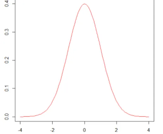
Let X be a continuous random variable whose law has the densityf defined onRby:
f(t) = √1
2πe
−1 2t
2 .
The function f is called density function of the reduced normal centered law denoted
N(0,1). It is a positive function.
Figure 1: Density of the Normal Law Centered Reduced
The curve above is a symmetrical curve with respect to the origin which has a bell-shaped shape. It is commonly called Gaussian curve.
The normal law is used in this subsection because it is the most commonly used prob-abilistic model to describe many phenomena observed in practice.
In what follows, we will generate the data from theRsoftware to show the influence of theh smoothing parameter in evaluating the performance of the circular kernel estimator. 8.2.1. Result of the simulation
For a sampleN = 500 , we assign the values to the smoothing parameter, which allows us to obtain the following curves:
For h= 2, we have the following curve:
For h= 1, we have the following curve:
Figure 3: Comparison of the theoretical curve and the kernel density estimator at h = 1
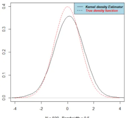
For h= 0.5, we have the following curve:
Figure 4: Comparison of the theoretical curve and the kernel density estimator at h = 0.5
For h= 0.3, we have the following curve:
For h=hopt, we have the following curve:
Figure 6: Comparison of the theoretical curve and the kernel density estimator ath=hopt
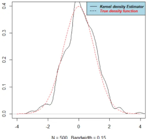
For h= 0.15, we have the following curve:
Figure 7: Comparison of the theoretical curve and the kernel density estimator at h=0.15
8.2.2. Interpretation
estimator, it is not the same for the smoothing parameter. A parameter that is too weak causes the appearance of artificial details appearing on the graph of the estimator. For a value ofh that is too large (see Figure 2, Figure 3), the majority of the characteristics are on the contrary erased. The choice of h is therefore a central question in estimating density. Hence the importance of determining an optimal smoothing parameter. The calculation of this optimal parameter gives us for a sample of sizeN = 500, hopt = 0.2587,
(see Figure 6). At this value, our estimator is almost similar to the true density, which shows us the efficiency of our estimator and so this estimator can therefore substitute for the density function of the reduced normal centered law.
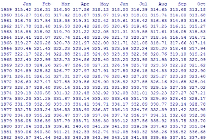
8.3. Real Data Case
In this subsection, we use data collected during a survey to study the concentration of CO2 in the atmosphere around a very active volcano called Mauna Loa in the Hawaiian
Archipelago in the United States of America culminating at 4, 100 meters above level. This study was conducted between 1959 and 1997 from January to December of those years of study. The catches below present all these data expressed in ppm (parts per million):
Figure 8: Concentration data inCO2 from January to October
In this study, 468 data was collected. The curve of the function of the reduced normal centered law for these real data is obtained through the software R:
Figure 10: True density function with real data
The curve of the density of the normal law above is positive and is taken in half. In what follows, we will generate the data from the Rsoftware
8.3.1. Result of Simulation
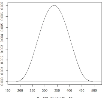
The simulation was performed for several values of the smoothing parameter. For h= 50,we have the following curve:
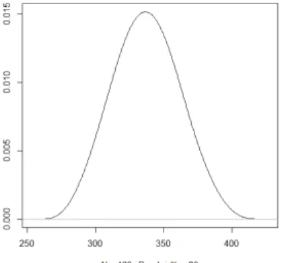
For h= 20,we have the following curve:
Figure 12: Curve of the kernel estimator for h = 20
For h= 10,we have the following curve:
Figure 13: Curve of the kernel estimator for h = 10
For h= 3,we have the following curve:
For h= 2,we have the following curve:
Figure 15: Curve of the kernel estimator for h = 2
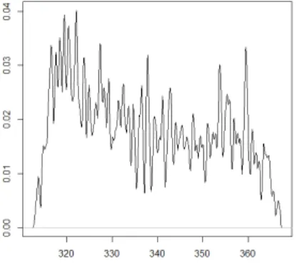
For h= 1,we have the following curve:
Figure 16: Curve of the kernel estimator for h = 1
8.3.2. Interpretation
As in the case of simulated data, according to different values of the smoothing param-eter,we have a curve which has a different look and tends to move away or closer to the true graph of the density function of the reduced normal centered law (see Figure 12 and Figure 13) represented under the basis of our 468 observations.
On the other hand, we found that at first, the density curve of the normal law is taken almost half (see Figure 10). And secondly, our different curves have several fluctuations and we observe rounded shapes of their representations (see Figure 14, Figure 15 and Figure 16), this is due to the fact that all the different data we are working on have very small values and so we have used a smaller scale.
non-parametric kernel-based estimators is closely related. Hence the importance is given to the determination of an appropriate smoothing window to remain in perfect adequacy in the handling of our raw data.
9. Conclusion and Perspectives
In this paper, we have established the bias and variance of circular kernel density. In addition, we have determined the optimal b∗n window of this estimator after first estab-lishing the mean squared error (MSE) and the mean integrated squared error (MISE) of this estimator. Finally, we have established the asymptotic expression of the bias of the circular kernel risk function estimator. This work is part of the continuity of the work of [18], [22] and [26] on the estimation of the survival function and the risk function in independent cases and identically distributed with and without censorship.
Through simulated data and real data, we have shown that the curve of the non-parametric estimator of the density function of the circular kernel is confounded with that for the optimal window this which proves the efficiency of our estimator.
However, some improvements remain to be done in this article. Indeed, it is a question of establishing the confidence intervals of the kernel estimator of the density function and the risk function of the circular kernel; to redo this work in the context of asymmetric nuclei and if possible to extend the study of the estimation of the conditional risk function in the case of the discrete nucleus.
Acknowledgements
The authors thank the reviewers of the European Journal of Pure and Applied Math-ematics for the contributions and suggestions they will make on this article.
References
[1] Odd Aalen. Nonparametric inference for a family of counting processes. The Annals of Statistics, pages 701–726, 1978.
[2] JR Blum and V Susarla. Maximal deviation theory of density and failure rate function estimates based on censored data. Multivariate analysis, 5:213–222, 1980.
[3] D Bosq and JF Lecoutre. ((th eorie de l’estimation fonctionnelle)) economica, 1987. [4] Antonia Foldes and Lidia Rejto. Strong uniform consistency for nonparametric
sur-vival curve estimators from randomly censored data. The Annals of Statistics, pages 122–129, 1981.
[6] Edward L Kaplan and Paul Meier. Nonparametric estimation from incomplete ob-servations. Journal of the American statistical association, 53(282):457–481, 1958. [7] John P Klein and Melvin L Moeschberger. Semiparametric proportional hazards
re-gression with fixed covariates.Survival analysis: techniques for censored and truncated data, pages 243–293, 2003.
[8] John P Klein and Melvin L Moeschberger. Survival analysis: techniques for censored and truncated data. Springer Science & Business Media, 2006.
[9] Jean-Pierre Lecoutre. Contribution `a l’estimation non param´etrique de la r´egression. PhD thesis, 1982.
[10] Jan Mielniczuk et al. Some asymptotic properties of kernel estimators of a density function in case of censored data. The Annals of Statistics, 14(2):766–773, 1986. [11] Elizbar A Nadaraya. On estimating regression. Theory of Probability & Its
Applica-tions, 9(1):141–142, 1964.
[12] Wayne Nelson. Theory and applications of hazard plotting for censored failure data.
Technometrics, 14(4):945–966, 1972.
[13] Didier Alain Njamen-Njomen and Joseph Ngatchou-Wandji. Nelson-aalen and kaplan-meier estimators in competing risks. Applied Mathematics, 5(04):765, 2014.
[14] DA Njamen Njomen. Convergence of the nelson-aalen estimator in competing risks.
International Journal of Statistics and Probability, 6(3):9–23, 2017.
[15] Didier Alain Njamen Njomen and Joseph Wandji Ngatchou. Consistency of the kaplan-meier estimator of the survival function in competiting risks.The Open Statis-tics & Probability Journal, 9(1), 2018.
[16] Didier Alain Njamen Njomen and Ludovic Kakmeni Siewe. A study of the ability of the kernel estimator of the density function for triangular and epanechnikov kernel or parabolic kernel. International Journal of Statistics and Applications, 9(2):45–52, 2019.
[17] Emanuel Parzen. On estimation of a probability density function and mode. The annals of mathematical statistics, 33(3):1065–1076, 1962.
[18] Henrik Ramlau-Hansen. Smoothing counting process intensities by means of kernel functions. The Annals of Statistics, pages 453–466, 1983.
[19] Murray Rosenblatt. Remarks on some nonparametric estimates of a density function.
The Annals of Mathematical Statistics, pages 832–837, 1956.
[21] Jeffrey S Simonoff. Smoothing Methods in Statistics. Springer Science & Business Media, 1996.
[22] Martin A Tanner and Wing Hung Wong. The estimation of the hazard function from randomly censored data by the kernel method. The Annals of Statistics, pages 989–993, 1983.
[23] Alexandre B Tsybakov. Introduction to nonparametric estimation, 2009. URL https://doi. org/10.1007/b13794. Revised and extended from the, 2004.
[24] Geoffrey S Watson. Smooth regression analysis. Sankhy¯a: The Indian Journal of Statistics, Series A, pages 359–372, 1964.
[25] GS Watson and MR Leadbetter. Hazard analysis. i. Biometrika, 51(1/2):175–184, 1964.