Improving Flow Lines by Unbalancing
Zsolt Mihály
Optasoft Kft., 1051 Budapest, Hungary
E-mail: [email protected], www.optasoft.hu Zoltán Lelkes
Department of Information Technology, Pallasz Athéné University, 6000 Kecskemét, Hungary E-mail: [email protected], www.uni-pae.hu
Keywords: flow line, throughput, cycle time, work-in-process Received: October 30, 2018
The paper's aim is to show how the performance of a balanced manufacturing flow line can be improved on the critical WIP level by making it unbalanced to some extent. The explanation and a quantitative example are presented. There is a trade-off between system balance and stability, and it can be handled as an optimization problem. Data are gathered using a physical simulation system. The analysis is carried out with a discrete time simulation program which applies next-event time advance mechanism. The model has been implemented in AIMMS modelling language.
Povzetek: V prispevku je prikazana uporaba rahle neuravnoteženosti pri kritičnih opravilih na sicer uravnoteženih opravilih tekočega traku. Model je bil implementiran v jeziku AIMMS in rezultat ovrednoten s pomočjo diskretne simulacije.
1
Introduction
The world makes great efforts to diminish the ecological footprint of humanity. For this reason, companies have to meet more and more regulations; corporations are forced to be more efficient. Thus, researches on environmentally benign business practices receive more and more attention [12]. One of the main interests is to improve production systems, like production of cars, pharmaceutical ingredients or electrical goods. It not only diminishes the ecological footprint, but also increases the profitability of the company by higher productivity, lower response time or lower inventory level.
Discrete manufacturing systems can be classified by several disciplines. Following Govil and Fu [4], the manufacturing systems can be
• job shops,
• flow lines,
• flexible manufacturing systems,
• assembly systems.
Manufacturing systems consist of stations. They are atomic processes, that is to say, they cannot be divided further. The main characteristic of a station is its process time. This is the time needed to process an entity. It is a scalar in a deterministic model, and a random variable in a stochastic model. In the latter case, process time has a
mean, a variance, and a type of probability distribution function.
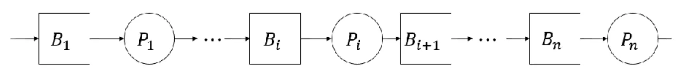
The research of manufacturing systems uses diverse modelling techniques, e.g., simulation models [13], queueing theory and Petri nets [9]. In this paper, flow lines are investigated using physical experiments and a discrete time simulation model. In flow lines, stations are connected in a linear way (see Figure 1). Some examples from the literature contain investigations into flow line with common buffer [16], complex optimization problems where the flow line is only one element in the model [8] or more complicated systems. Huang and Li examined a two-stage hybrid flow shop with multiple product families [7]. Simulation modelling has a wide range of applications in engineering-aided manufacturing regarding system performance. Modelling apparel assembly cells [1], a Mercedes-Benz production facility [10], or analysing the performance of a Korean motor factory [2] are only some of the examples.
Hopp and Spearman [6] investigated flow lines in which there is only one machine per station, one job class, no capacity constraint, and the queueing principle is first in, first out (FIFO). Three main modelling measures are proposed by them:
• Throughput (TH): the number of entities (cars, apples, people, etc...) coming out from the system during a given time
• Cycle time (CT): the time an entity spends in the system
• Work-in-process (WIP): the number of entities residing in the system at the same time
The system performs better if it has a higher TH or a lower CT. These parameters are not independent from each other. Little's law makes a connection among them:
𝑊𝐼𝑃 = 𝑇𝐻 × 𝐶𝑇
According to the previous equation, the optimal value of WIP in a deterministic system is
𝑊0= 𝑇0× 𝑟𝑏
Where
• Bottleneck rate (𝑟𝑏): the rate of the station that has the highest utilization
• Raw process time (𝑇0): the sum of the average process times in the flow line
• 𝑊0 is called the critical WIP level ([6]).
The variability of procedures is measured with the coefficient of variation (CV):
𝐶𝑉 =𝑠𝑡𝑎𝑛𝑑𝑎𝑟𝑑 𝑑𝑒𝑣𝑖𝑎𝑡𝑖𝑜𝑛 𝑚𝑒𝑎𝑛
Hopp and Spearman use two so called characteristic functions to analyse the performance. The dependent variables are the TH and the CT, while the independent variable is the WIP level both times. The flow line is modelled as a closed network. It means that the level of WIP is a model parameter [14]. Regarding performance analysis, three important concepts were introduced [6]:
Best case performance: the best possible performance for a line. It is balanced, and there is no batching.
Worst case performance: the worst possible performance for a line. All the entities move in one batch. Practical worst case (PWC): as the worst case performance is so bad that it is far from practical instances, PWC was introduced to define a realistic worst case.
The paper's aim is to show how the performance of a balanced manufacturing flow line can be improved on the critical WIP level by making it unbalanced to some extent. The explanation and a quantitative example are presented. There is a trade-off between balance and stability, and it can be handled as an optimization problem.
2
Method of examination
In this research, the same characteristics are used to evaluate the performance as in [5]. Both physical and simulation model experiments are performed to gather data. Both models are flow lines with FIFO queueing discipline containing single machine stations, one job class and using constant work-in-process (CONWIP) control. It means that a new entity arrives into the system only when another one leaves it.
In the physical model experiment, a toy car factory has been realized with the assumption of infinite raw material stock. The entire process to build a small car takes 4 minutes. In an arbitrary way, the operations could be distributed among 4 production processes where one-one person works with different abilities. Beside the four production processes, there is a transport process as well. Altogether there are 5 stations.
Building a simulation model consists of three levels. There is a superstructure which can represent all the possible flow lines. Beside this, there is a mathematical model and an algorithm. Based on the algorithm, a discrete time simulation program with next-event time advance mechanism is worked out. Comparing with fixed-increment time advance method, it is more complicated, but more efficient regarding computational need [15].
The simulation program is implemented in AIMMS modelling language [11]. It has already been used in other studies with success. E.g., [3] used it on supply chain optimization with homogenous product transport constraints. The simulation program can be easily extended in this environment. AIMMS is linked to the most modern solvers, which are easily integratable. Furthermore, it has an advanced graphical user interface, which can be used for creating simply usable and ergonomic softwares.
3
Results
3.1
The explanation of the trade-off
Regarding a given raw process time (𝑇0), a deterministic balanced line performs better than a deterministic unbalanced line. On the other hand, the balanced line has a worse stability regarding variability [6] .
Let us investigate a balanced system whose raw process time is 𝑇0, and has n stations. It is true in this case that
∀𝑖 𝑇𝑖= 𝑇0
𝑛
(𝑇𝑖 denotes the average process time of the i-th station) That is to say, all the process times are the same. So the bottleneck rate:
𝑟𝑏 = 𝑛 𝑇0
If the system with the raw process time 𝑇0 is unbalanced then
∃𝑖 𝑇𝑖> 𝑇0
𝑛
From this, it can be concluded that for the unbalanced system
𝑟𝑏 < 𝑛 𝑇0
The TH of a deterministic system is calculated in the following way:
The two systems have the same performance until 𝑊𝐼𝑃 ≤ 𝑟𝑏𝑇0
After that the balanced system works better because it has a higher 𝑟𝑏. This proves that a balanced line has a better performance in this case
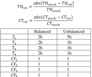
It is harder to prove mathematically that a balanced line is less stable. Nonetheless, this effect could be seen when investigating the physical model. In this section, an example is shown. Two flow lines are compared. For both of them, 𝑇0= 8ℎ, and each of them contains four stations. In the balanced line
∀𝑖 𝑇𝑖= 2ℎ
In the unbalanced line, the first station is the bottleneck, its process time is 5h, and 1h regarding the rest of them. In the stochastic case for both systems
∀𝑖 𝐶𝑉𝑖= 1
The characteristics of the flow lines are summed up in Table 1.
The results of the experiment can be seen in Figure 2. Relative changes are displayed on the ordinate, which shows the deteriorating effect of variability from a different aspect as usual characteristic functions. The reason for applying it is that it is easier to see the difference in the drop of performance regarding WIP. These characteristics are calculated in the following way.
𝑇𝐻𝑟𝑒𝑙 =
𝑎𝑏𝑠(𝑇𝐻𝑠𝑡𝑜𝑐ℎ− 𝑇𝐻𝑟𝑒𝑙) 𝑇𝐻𝑠𝑡𝑜𝑐ℎ
𝐶𝑇𝑟𝑒𝑙=
𝑎𝑏𝑠(𝐶𝑇𝑠𝑡𝑜𝑐ℎ− 𝐶𝑇𝑟𝑒𝑙) 𝐶𝑇𝑠𝑡𝑜𝑐ℎ
Balanced Unbalanced
𝑇1 2h 5h
𝑇2 2h 1h
𝑇3 2h 1h
𝑇4 2h 1h
𝐶𝑉1 1 1
𝐶𝑉2 1 1
𝐶𝑉3 1 1
𝐶𝑉4 1 1
Table 1: The characteristics of the investigated flow lines Both of the diagrams show that the extent of deterioration is bigger when the line is balanced. In this case, the maximal TH decrease is 42% in the balanced system, and 18% in the unbalanced one. The maximal CT increase is 73% when the flow line is balanced; 22% when it is unbalanced. It means that the maximal deterioration of TH is twice as high in balanced lines as in unbalanced lines, and the maximum of CT deterioration is three times as high. That is, evidence is shown that balanced line has less stability regarding variability. The same phenomena could be observed in each physical experiments. The loss of TH and the growth of CT increase until the critical WIP value is reached. After the peak, both functions begin to decrease. At high WIP levels, they will converge into 0. Table 2 sums up the results regarding the peaks.
a) Decrease of TH
b) Increase of CT
Figure 2: The stability of flow lines regarding variability Balanced Unbalanced
TH 42% 18%
CT 173% 122%
Table 2: Comparison of the maximal deteriorations
3.2
A quantitative example for system
unbalancing
In this section, a quantitative example is shown in which the unbalanced system has a better performance on the critical WIP level. Three systems are compared: a balanced and two unbalanced. The balanced system has uniform process times of 1 hour. The CV of the first three stations are equal to 0.1, and the last station's CV is 1. In the unbalanced systems, the process times of three operations are 1.15 hour, and there is one with 0.55 hour. That is, they differ in the position of the non-bottleneck process. The station with the process time of 0.55 hour has CV = 1. The CV of the bottlenecks are 0.1. The characteristics of the investigated systems can be seen on Table 3.
0 5 10 15 20 25 30 35 40 45
1 3 5 7 9
Rela
tive
T
H d
e
cr
e
a
se
[%
]
WIP [-]
Balanced Unbalanced
0 10 20 30 40 50 60 70 80
1 3 5 7 9
Rela
tive
CT
in
cr
e
a
se
[%
]
WIP [-]
Balanced
Unbalanced (first three are
bottlenecks)
Unbalanced (last three are
bottlenecks)
𝑇1 1h 1.15h 0.55h
𝑇2 1h 1.15h 1.15h
𝑇3 1h 1.15h 1.15h
𝑇4 1h 0.55h 1.15h
𝐶𝑉1 0.1 0.1 1
𝐶𝑉2 0.1 0.1 0.1
𝐶𝑉3 0.1 0.1 0.1
𝐶𝑉4 1 1 0.1
Table 3: The characteristics of the investigated flow lines. The critical WIP level of the flow line can be calculated in the following way:
𝑊0= 𝑟𝑏× 𝑇0= 1 1
ℎ× 4ℎ = 4
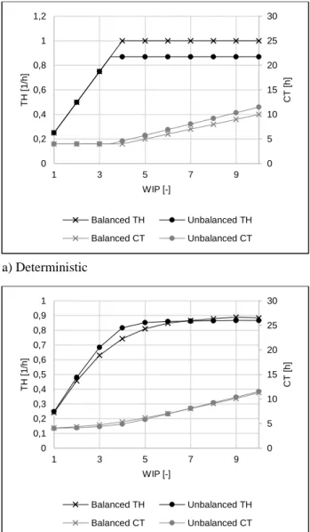
The positions of the bottleneck procedures have no effect in the unbalanced systems (Figure 3/b, 3/c). In the deterministic case, the balanced system performs better, as expected. On the other hand, when there is variability, the unbalanced flow line has a better output on the critical WIP level (see Table 4, 5). According to the experiments, the TH of the unbalanced system can be 9-11% higher compared with the balanced line, the CT is 8-9% lower. The results confirm the assumption that there is a trade-off between balance and stability, and it can be handled as an optimization problem.
Balanced Unbalanced
TH [1/h] 1 0.87
CT [h] 4 4.6
Table 4: the performance of the investigated system on the critical WIP level in the deterministic case
Balanced Unbalanced Improvement TH 0.74 1/h 0.82 1/h 11%
CT 5.38 h 4.90 h 9%
Table 5: the performance of the investigated system on the critical WIP level in the stochastic case
4
Conclusion
Endeavours are generally made to balance flow lines. This is an intuitive idea, and earlier researches showed examples where unbalanced systems had worse performance. In this paper, it has been shown that unbalancing the flow line in a small extent achieves better performance on the critical WIP level, that is to say, higher TH and lower CT. In the examined case, the TH was 9-11% higher and the CT 8-9% lower on the critical WIP level.
This result is important in flow lines as well where the manufacturing is precise, but there are several products. Each of them might have a low variability, but the variability of the stations’ process times can be high if the average process times of products are different.
a) Deterministic
b) Stochastic (First three processes are bottlenecks)
c) Stochastic (Last three processes are bottlenecks) Figure 3: Comparison of the performance of a balanced and two unbalanced systems.
0 5 10 15 20 25 30 0 0,2 0,4 0,6 0,8 1 1,2
1 3 5 7 9
CT [ h ] T H [1 /h ] WIP [-]
Balanced TH Unbalanced TH
Balanced CT Unbalanced CT
0 5 10 15 20 25 30 0 0,1 0,2 0,3 0,4 0,5 0,6 0,7 0,8 0,9 1
1 3 5 7 9
CT [ h ] T H [1 /h ] WIP [-]
Balanced TH Unbalanced TH
Balanced CT Unbalanced CT
0 5 10 15 20 25 30 0 0,1 0,2 0,3 0,4 0,5 0,6 0,7 0,8 0,9 1
1 3 5 7 9
CT [ h ] T H [1 /h ] WIP [-]
Balanced TH Unbalanced TH
List of symbols
CT Cycle time
TH Throughput
WIP Work-in-process 𝑇0 Raw process time 𝑟𝑏 Bottleneck rate 𝑊0 Critical WIP level
𝑇𝑖 Average process time at station i 𝐶𝑉𝑖 Coefficient of variability at station i
n Number of stations
References
[1] J. T. Black and B. J. Schroer. Simulation of an apparel assembly cell with walking workers and decouplers. Journal of Manufacturing Systems, 12(2):170-180, 1993.
https://doi.org/10.1016/0278-6125(93)90016-M [2] K. Cho, I. Moon, and W. Yun. System analysis of a
multi-product, small-lot-sized production by simulation: A Korean motor factory case. Computers & Industrial Engineering, 30(3):347-356, July 1996. https://doi.org/10.1016/0360-8352(96)00003-4 [3] T. Farkas, Z. Valentinyi, E. Rév, and Z. Lelkes.
Supply chain optimization with homogenous product transport constraints. In Computer Aided Chemical Engineering, volume 25, pages 205-210, 2008. https://doi.org/10.1016/S1570-7946(08)80039-9 [4] M. Govil and M.C.Fu. Queueing theory in
manufacturing: A survey. Journal of Manufacturing Systems, 18(3):214-240, 1999.
https://doi.org/10.1016/S0278-6125(99)80033-8 [5] W. J. Hopp. Supply Chain Science. Waveland Pr Inc,
Long Grove, Illinois, 2011.
[6] W. J. Hopp and M. L. Spearman. Factory Physics. McGraw-Hill Education, New York, New York, 2000. https://doi.org/10.1036/0256247951
[7] W. Huang and S. Li. A two-stage hybrid flowshop with uniform machines and setup times. Mathematical and Computer Modelling, 27(2):27-45, January 1998.
https://doi.org/10.1016/S0895-7177(97)00258-6 [8] J. Olhager and B. Rapp. Balancing capacity and lot
sizes. European Journal of Operational Research, 19(3):337-344, March 1985.
https://doi.org/10.1016/0377-2217(85)90130-4 [9] H. T. Papadopoulos and C. Heavey. Queueing theory
in manufacturing systems analysis and design: A classification of models for production and transfer lines. European Journal of Operational Research, 92(1):1-27, July 1996.
https://doi.org/10.1016/0377-2217(95)00378-9 [10] Y. H. Park, J. E. Matson, and D. M. Miller.
Simulation and analysis of the Mercedes-Benz all activity vehicle (aav) production facility. In Proceedings of the 1998 Winter Simulation Conference, pages 921-926, December 1998. https://doi.org/10.1109/WSC.1998.745790
[11] M. Roelofs and J. Bisschop. AIMMS The user's guide. AIMMS B.V., AP Haarlem, The Netherlands, 2016.
[12] J. Sarkis. A strategic decision framework for green supply chain management. Journal of Cleaner Production, 11(4):397-409, June 2003.
https://doi.org/10.1016/S0959-6526(02)00062-8 [13] J. S. Smith. Survey on the use of simulation for
manufacturing system design and operation. Journal of Manufacturing Systems, 22(2):157-171, 2003. https://doi.org/10.1016/S0278-6125(03)90013-6 [14] W. Whitt. Open and closed models for networks of
queues. AT&T Bell Laboratories Technical Journal, 63(9):1911-1979, November 1984.
https://doi.org/10.1002/j.1538-7305.1984.tb00084.x [15] W. L. Winston. Operations Research: Applications and Algorithms. Cengage Learning, Boston, Massachusetts, 2003.
[16] H. Yamashita and S. Suzuki. An approximation method for line production rate of a serial production line with a common buffer. Computers & Operations Research, 15(5):395-402, 1988.