Open Journal Systems

(1)

Hungarian Association of Agricultural Informatics European Federation for Information Technology in Agriculture, Food and the Environment

Journal of Agricultural Informatics. Vol. 7, No. 1 journal.magisz.org

Performance of Sentinel-2 data in unsupervised classification: a case study of

statistical comparison with Landsat 8 OLI

Györk Fülöp1_,

I N F O

Received 16 Mar. 2016 Accepted 11 Apr. 2016 Available on-line 30 Apr. 2016 Responsible Editor: M. Herdon

Keywords:

Sentinel-2, performance, landscape indices, spatial pattern, multivariate statistics

A B S T R A C T

What to expect, when planning to use Sentinel-2 datasets in unsupervised classification? This is a very actual question, since Copernicus Sentinel-2 data has been available since November 2015, but due to the winter period conditions, wide use has been obstacled, user experiences are missing. In a European Space Agency (ESA) financed feasibility study we needed to simulate 2015 Sentinel-2 data input with Landsat 8 OLI data, and we were also curious, how this may affect the performance? In a case study we measured Sentinel-2 and Landsat-8 OLI to Kompsat-3 very high resolution multispectral imagery in four sample sites and we used landscape indices to quantify the effect of utilized input data on spatial pattern.

1. Introduction

In the confines of a European Space Agency (ESA) financed feasibility study (contractor: GeoData Services Ltd.), three Copernicus Sentinel data based Earth Observation service developments has been prepared for launch and were examined from a technical aspect. During the feasibility study we needed to use Landsat 8 OLI (L8) data simulating Sentinel-2 (S2) data input. In my task group we also carried out a small experiment to interpret how will real S2 data (ESA 2016) based service quality differ from the recent L8 (USGS 2015) supported results. The outcomes may be of interest of many, since S2 data had already been published via the Sentinel Scientific Data Hub since November 2015, but due to the weather conditions of the winter period operative, take-up has been hindered.

Our experiment was designed to have an empirical approach: we were interested how the unsupervised classification of only one image of S2 is influenced by the data quality? Thus, at the very first moment we ruled out one of the most important new quality of S2: its increased revisit frequency (S2: 5 days; L8: 16 days). In the study we also did not assess the performance of the access facilities (S2: Scientific Data Hub; L8: USGS Earth Explorer), effective data sizes, formats and primer infrastructures of the data platforms.

Our practical approach was to identify with multivariate statistics how the utilized input data affect the resulted spatial pattern of the unsupervised classification. Thus our objective was analogue to a variance analysis: to delineate the statistical power of utilized sensors on resulted spatial pattern from other effects. The analysis can be automated and executed with other input datasets as well, thus it can be taken as a case study of a frame work intention to qualify single image performance of remotely sensed data.

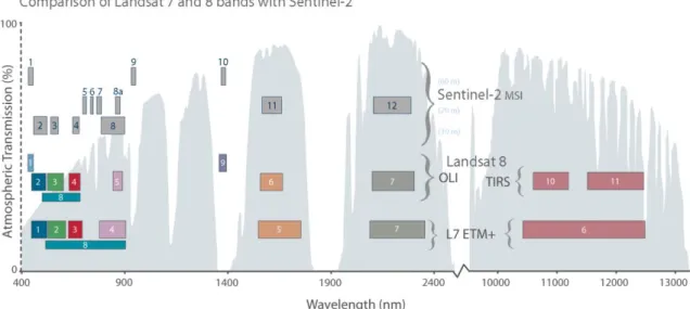
Before giving a short summary of the experiment setup, the calculations and the results, the performance influencing metadata shall be described here. Besides the radiometric layout of the datasets (Figure 1) phargitai, S2 provides the 13-band spectral data in three different spatial resolutions (10 m: Band 2-4, 8; 20 m: Band 5-8a; 11-12; 60 m: Band 1, 9, 10), while L8 provides the multi spectral information in two spatial resolutions (30 m: Band 1-7, 9; 100 m: Band 10-11) and one panchromatic band (Band 8: 15 m). Over the sample sites L8 has its pass at 9:27, S2 at 10:02 CET.

1_{Györk Fülöp}

(2)

Figure 1. Setup of Sentinel-2 and Landsat 7-8 HR multispectral bands (source of imagery: http://earth.esa.int)

2. Experiment setup – data and samples

The experiment was set up, measuring the performance of S2 and L8 high resolution imagery to a Kompsat-3 (K3) very high resolution reference image (EOPORTAL 2016). The reference image was taken 26.04.2013. In the study only the 4-band multispectral (4 m) data were used (B: 450-520 nm; G: 520-600 nm; R: 630-690 nm; NIR: 760-900 nm), 1 m panchromatic information was excluded.

First challenge of the experiment setup was to find spatially with the K3 reference imagery overlapping S2 and L8 imagery, with decent cloud cover and in time close to each other. After researching in the Sentinel Scientific Data Hub (SCIHUB 2016) and the USGS Earth Explorer (EARTHEXPLORER 2016) catalogues, a 14.01.2016 (S2) – 20.01.2016 (L8) data pair seemed to be adequate for the experiment.

S2 and L8 input data originating from the winter period (less vegetation) might influence the expected multispectral quality of the images significantly (E.g.: precision approach of S2 NIR bands might not be represented with enough power), but this discrepancy shall be ruled out by the fact that both S2 and L8 image sets are from close range in time, and that a preliminary report shall present what to expect in the active imaging period of 2016 already. However, the reference K3 image was taken almost three years earlier, showing mid-spring vegetation. With this, we arrive to the second challenge: such sample sites had to be defined in the images, where significant changes are not likely to happen.

(3)

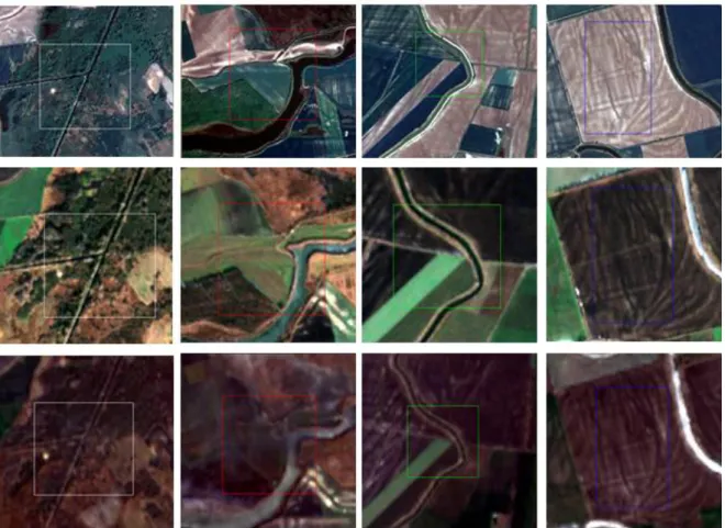
Figure 2. Sample sites; from right to left NO1-NO4; from up to down on K3-S2-L8 RGB composites It might be observed, that the primer diversity of the samples is decreasing from NO1 to NO4, while NO1-2 are basically of the same extent, NO3 is of a small extent sampling, NO4 is of a huge extent agricultural parcel, representing only bare soil (Figure 3).

Figure 3. Situation of sample sites in Google Earth with thumbnail of S2 Band-4 data; yellow AOI:

(4)

3. Primer image processing

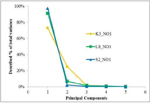
During the primer image processing we processed the input (K3, S2, L8) imagery in parallel, to achieve datasets, which can be compared to each other efficiently. During the data processing ENVI 4.7 software [1] were utilized, thus all input data was converted into ENVI .hdr format. As preliminary steps, L8’s B1-7 multispectral bands were pan-sharpened (with Band 8) and S2 bands were resampled (nearest neighbour), all to have 10 m resolution. Then, multispectral stacks were created from K3 (4 bands), S2 (13 bands) and L8 (7 bands) data. After subsetting the stacked imagery with sample AOIs, each sample were over-sampled (1 m) using cubic convolution method. After achieving uniform virtual spatial resolution, to handle the different numbers of input bands (which may influence the unsupervised classification), all samples (K3, S2, L8) were undergoing a Principal Component Analysis (PCA), and in each cases the first 3-3 PCs were saved as independent bands of a stack. 3rd PCs were preserved only for safety reasons (not to lose different amount of information), since in all samples the first two PCs described the original input with convincing power (Figure 4).

Figure 4. PCA performance in case of NO1 (K3, S2, L8)

(5)

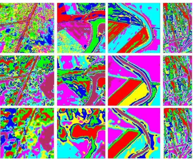
Figure 5. K-mean classified sample sites; from right to left NO1-NO4; from up to down resulted from K3-S2-L8 data input

4. Secondary image assessment

The secondary image assessment was aiming to compare the resulted classified data statistically. The difference in the resulted class-structure can be the effect of 1) error of experiment: effective changes on the surface between acquisitions; 2) effect of sensor: difference between information contain of S2 and L8 HR and K3 VHR image acquisitions; 3) effect of sites: different attributes and spatial structure of sample sites.

To gain numeric description of classified imagery, the GeoTiff sets were ingested into Fragstats 4.2 software [2] to assess their spatial pattern. During the automatic assessment, adjacency tables and landscape (sample) level statistics were created in table format. Landscape indices were computed to describe the 1) classified samples’ area and edge relations; 2) the contained patches’ shape; 3) the spatial distribution of the patches (aggregation); and 4) the landscape diversity of sample sites. Used landscape indices are presented in Table 1, with respect to their known computation and meaning (MCGARIGAL 2015).

Table 1. Applied landscape level statistics

Index group Area and edge Shape Aggregation

Diver-sity Indices AR E A L PI

TE GYRATE SHAPE PAR

(6)

It must be emphasized, that landscape metrics are not utilized in this study in their general function – to support landscape ecological and landscape planning decision making, but as mirrors of the affects, which are created by differently sensed data. This consideration gives excuse of GUSTAFSON’s

(1998) in general very accurate and valid observation on the false interpretation of landscape indices. Landscape metrics are not interpreted, only used for measuring underlying effects, thus the causal direction is opposite.

5. Results and discussion

Statistical assessment of output adjacency tables and landscape level statistics were executed in three phases. First, autocorrelation information was extracted from adjacency relations, then landscape index values were undergoing dimension reduction, finally a general linear model was used to describe the relations between the sample sites, and to define the force of utilized datasets on the spatial differences. For statistical analysis IBM SPSS Statistics 20.0 was used [3].

5.1. Assessment of classification resulted adjacency: autocorrelation for image performance

Adjacency describes a categorical map, how the neighbourhood relations of the rasters of a given class are distributed among all the classes. In Table 2 the adjacency matrices of the first sample site can be seen, as observed on the categorical maps extracted from K3, L8 and S2 data. When first observing the adjacency matrices, it can be noticed, that cells are organized symmetrically along the main diagonal of the matrix. It can also be observed, that the values of the cells are not distributed the same way, VHR K3 data resulted adjacency is expending further from the diagonal, than HR resulted adjacencies.

Table 2. Adjacency matrices of the sample site NO1, resulted from K3, L8 and S2 input data

K3_NO1

Class ID 1 2 3 4 5 6 7 backgr.

1 161230 14955 25 9 0 0 0 181

2 14955 495258 4017 37684 218 3 0 513 3 25 4017 227254 1931 6996 0 927 234 4 9 37684 1931 516116 31110 12597 1 736 5 0 218 6996 31110 326358 25637 2901 712 6 0 3 0 12597 25637 403620 13770 677 7 0 0 927 1 2901 13770 143914 163

L8_NO1

1 349056 9244 0 0 0 0 0 436

2 9244 524382 5251 5125 0 0 0 854 3 0 5251 344422 3502 3510 0 0 475 4 0 5125 3502 350214 7341 0 0 330 5 0 0 3510 7341 378316 7630 0 455

6 0 0 0 0 7630 328934 3389 447

7 0 0 0 0 0 3389 252252 243

S2_NO1

1 254434 9834 0 0 0 0 0 256

2 9834 528506 18411 1 0 0 0 792

3 0 18411 391558 18098 2 0 0 431

4 0 1 18098 327942 16376 0 0 519

5 0 0 2 16376 334952 12301 0 517

6 0 0 0 0 12301 317324 5924 419

(7)

When considering the meaning of adjacency, we can relate to spatial similarity, and after a short thinking also to autocorrelation. Autocorrelation is a phenomenon, which results that spatially close objects are more likely to be similar (LABOVITZ et al. 1980, ODLAND 1988). Autocorrelation is more valid in datasets with coarser spatial resolution (DORMANN et al. 2007). If in an adjacency matrix the values of the cells are organized more and more “leaning” to the diagonal, the class-member rasters are more and more likely to be neighboured by class-members of similar clusters. But how to interpret adjacency matrices in order to extract the degree of autocorrelation?

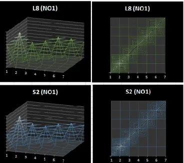
Figure 6. Surface and contour line representation of adjacency matrices of NO1 sample site

On Figure 6 surface model of adjacency table and contour line representation of adjacency relations can be seen (surface model from above). Unfortunately, even though that it describes the distributions (among classes) expressively, degree of autocorrelation cannot be observed sufficiently. A matrix transformation is needed, which gives a view of the cross-section of the introduced surfaces – with a square root transformation in favour of interpretability (Figure 7).

The “sharpness” of the averaged adjacency cross-section can describe the autocorrelation relations, thus skewness can be a well-tailored index. Figure 8 shows the measured skewness information of the adjacency matrixes, thus the degree of autocorrelation in the categorical maps of K3, S2 and L8 input data. This way, skewness of adjacency – thus degree of autocorrelation – shows how the details get lost due to the resulting data, describing the phenomena in one index, handling the effects of spatial and spectral resolution together.

(8)

Figure 8. Skewness of adjacency surfaces – a possible measure for autocorrelation

It can be observed, that the 4-band VHR K3 has at all four sample sites the lowest skewness value – thus in this data it is more likely that a given raster is neighboured by rasters of other classes (in the 1 m resampled data based categorical maps). Skewness of S2 is in between K3 and L8 values, thus Sentinel-2 data gives measurably more detailed information of the Earth surface, than Landsat 8 OLI. Power of autocorrelation can be observed best on samples with extreme primer diversity (NO1 and NO4), where the spatial resolution of initial input datasets has greater significance.

With greater number of samples – thus more detailed diversity set up – the force of spectral and spatial resolution contributing to observable autocorrelation might be extracted and quantified separately with tests of variances.

5.2. Dimension reduction of resulted landscape index values

It would be a target of a landscape ecological study to measure how utilized input data can effect individual landscape indices and to explain its consequences on resulted decision support (WALTZ

2011). Recent study is aiming to quantify how the three different sensors (the reference VHR K3 and the tested HR S2 and L8) affect the index groups, thus area and edge relations, the shape attributes, the aggregation of patches and measurable landscape diversity. With this consideration, dimension reduction of measured index values was needed.

Principal component analysis was performed on index groups, compacting the indices into one PC in each cases (Table 3) using regression method for factor scoring. That it was possible to do so, highlights the problem of correlating landscape metrics, which issue was raised already by GUSTAFSON (1998).

Table 3. PCA of index groups AREA

indices

SHAPE indices

AGGREG. indices

L. DIVERS. indices

PC containing % of variance 82,08% 87,58% 77,32% 99,60%

Number of indices 4 4 5 2

Min of communalities 76,81% 73,33% 56,77% 95,98%

Index of min. comm. LPI SHAPE ENN SHDI=SIDI

Max. force component 0,9333 0,9647 -0,9682 0,9980

(9)

5.3. Explanatory statistics, force of input data, S2 performance

A General Linear Model (GLM) was built of independent variables of sensor (K3, S2, L8) and site (NO1-4) to describe how the depending factor scores of landscape indices are influenced by them. In the model, the sensor was kept to be the fixed factor (planned effect) and site information to be the random factor, while the landscape index resulted factor scores the dependent variables. The model was designed to assess how the variances of the measured landscape index factor scores are explained by the fixed factor (sensor), the random factor (site) and their intercept, and which part is inexplicable (error) (Table 4).

Table 4. The factors’ explained % variance by index groups; force of effects

AREA SHAPE AGGREG DIVERSITY

SENSOR 50,42% 92,92% 72,45% 2,93%*

SITE 45,59% 6,04%* 21,87%* 78,68%

ERROR 4,00% 1,03% 5,68% 18,39%

* significance level above 0,05

Since the intercept elements of the models were not significant in any cases, they were excluded from the model. Table 4 also represents the factors’ force to affect the spatial structure of the sample sites. As it can be seen, in case of area, shape and aggregation relations, the applied input data (sensor) affects with more force the measured landscape metrics, then the sites themselves. In case of the two diversity metrics (SHDI and SIDI) the ratio is opposite, site has more influence on the metrics, however inexplicable error has also increased value.

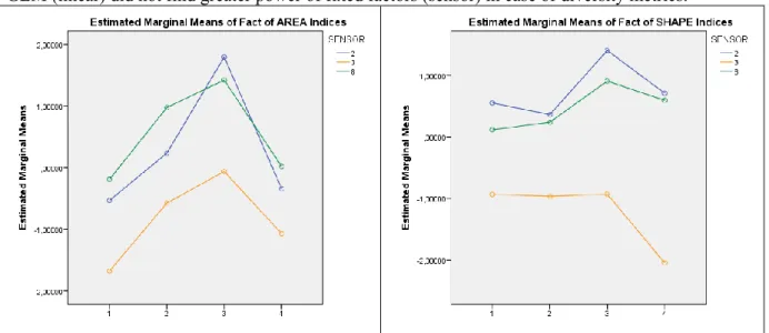
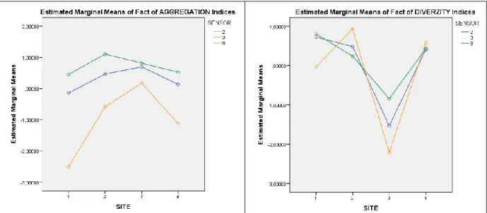
After the fixed (sensor) and random (site) factors were pruned of their co-effect (intercept) marginal means could be estimated. Figure 9-10 presents the marginal means of factor scores among sites by sensors. It can be observed that in case of area and edge metrics (except NO3 site) and aggregation metrics Sentinel-2 resulted index values is more close to the reference Kompsat-3 VHR image than values extracted out of Landsat 8 OLI data. In case of shape metrics Landsat-8 data input performs better than Sentinel-2. In case of diversity metrics the picture may be confusing, but after short examination it can be observed that K3 is taking the most extreme values (sensitive), while L8 is the most mediocre (generalizing). S2 falls in between K3 and L8. This can also be the reason why the GLM (linear) did not find greater power of fixed factors (sensor) in case of diversity metrics.

(10)

Figure 10. Estimated marginal means of the landscape metric based factor scores of aggregation and diversity metrics; sensor type: 2 (S2), 3 (K3), 8 (L8)

Table 5. Estimation of S2 performance from marginal means by landscape index groups Marg. mean

Sensor AREA SHAPE AGGREG DIV

K3 -0,847 -1,219 -1,010 -0,181

S2 0,289 0,756 0,288 0,022

L8 0,557 0,463 0,722 0,158

Marg. mean distance from reference K3

S2 1,136 1,603 1,134 0,869

L8 1,404 1,310 1,569 1,005

Marg. mean distance in % of L8

S2 80,93% 122,37% 72,29% 86,49%

L8 100,00% 100,00% 100,00% 100,00%

Perfromance of S2 measured to L8

S2 123,57% 81,72% 138,33% 115,62%

(11)

Figure 11. Performance of S2 in the percentage of L8 in reference to K3

When interpreting results presented in Figure 10, the validity of the outcomes must be questioned also by a landscape ecologist approach. Eg.: what plausibility the under-performing of patch shape detection has, when area and edge, aggregation and diversity indices show a significant difference? These questions must be raised in a separate study, which reaches out also to the interpretation of resulted index values.

6. Summary

In this paper a study has been presented, which aimed to compare the performance of unsupervised classification of high resolution multispectral Sentinel-2 and Landsat 8 OLI datasets with a reference to very high resolution multispectral Kompsat-3 imagery provided categorical maps. After the set-up of the experiments, spatially and timely overlapping imagery (reference imagery acquisitioned almost 3 years earlier) were gathered, comparable AOIs were defined. Primer image processing was applied to each dataset in parallel resulting comparable categorical maps. The statistical comparison utilized adjacency information for presentation of autocorrelation and compared spatial pattern of categorical maps with the help of landscape index groups (area and edge, shape, aggregation and diversity) on landscape (sample) level. The study resulted that the choice of input data has a significant force on the resulted spatial pattern, and that – in general – Sentinel-2 data performs better (measured to VHR reference) than Landsat 8 imagery. Degree of developed performance quality has been published, with remarks that landscape ecological approach shall interpret the long term edification of data utilization.

7. Acknowledgements

The study was carried out in the confines of MODE-EO project, funded by the Government of Hungary through an ESA Contract under the PECS (Plan for European Cooperating States). The view expressed herein can in no way be taken to reflect the official opinion of the European Space Agency.

(12)

References

DORMANN C.F., MCPHERSON J.M., ARAUJO M.B., BIVAND R., BOLLIGER J., CARL G., DAVIES R.G., HIRZEL A., JETZ W., KISSLING W.D., KÜHN I., OHLEMÜLLER R., PERES-NETO P.R., REINEKING B., SCHRÖDER B., SCHURR

F.M., WILSON R. (2007): Methods to account for spatial autocorrelation in the analysis of species distributional

data: a review. Ecography 2007 30 doi: 10.1111/j.2007.0906-7590.05171.x pp. 609-628.

EARTHEXPLORER (2016): USGS EarthExplorer [on-line] http://earthexplorer.usgs.gov/ [access: 08:13 14.03.2016]

EOPORTAL (2016): KOMPSAT-3 (Korea Multi-Purpose Satellite-3)/Arirang-3 [on-line]

https://directory.eoportal.org/web/eoportal/satellite-missions/k/kompsat-3#overview [accessed: 14.03.2016]

ESA (2016): SENTINEL-2 MSI Introduction [on-line] https://sentinel.esa.int/web/sentinel/user-guides/sentinel-2-msi [access: 14.03.2016]

GUSTAFSON E.J. (1998): Quantifying Landscape Spatial Pattern: What is the State of Art? Ecosystems. Springer 1998 1 pp. 143-156. doi: 10.1007/s100219900011

LABOVITZ M.L., TOLL D.L., KENNARD R.E. (1980): Preliminary evidence for the influence of physiography and

scale upon the autocorrelation function of remotely sensed data; NASA TM 82064; Goddard Space Flight

Center; Greenbelt; MD

MCGARIGAL K. (2015): FRAGSTATS 4.2 Help [on-line]

http://www.umass.edu/landeco/research/fragstats/documents/fragstats.help.4.2.pdf [access: 9:15 12.03.2015]

ODLAND J. (1988): Spatial autocorrelation. Sage Publications, California, 1988 ISBN: 0-8039-2652-9 pp. 15.

SCIHUB (2016): Sentinel Scientific Data Hub [on-line] https://scihub.copernicus.eu/dhus/#/home [access: 07:21 16.03.2016]

USGS (2015): Landsat 8 [on-line] http://landsat.usgs.gov/landsat8.php [last edited: 12.01.2015]

WALTZ U. (2011): Landscape Structure; Landscape Metrics and Biodiversity. Living Rev. Landscape Research. 2011 5(3) ISSN 1863-7329 doi: 10.12942/lrlr-2011-3