thesis.pdf

Magnet Simulations for ABRACADABRA

Chiara P. Salemi

Senior Honors Thesis

Department of Physics and Astronomy

University of North Carolina at Chapel Hill

March 27, 2017

Abstract

Contents

1 Introduction 2

2 Theoretical Background 4

3 ABRACADABRA 6

4 Simulation 8

4.1 Motivation and Considerations . . . 8

4.2 Methods . . . 10

4.2.1 Basic model . . . 10

4.2.2 Continuously wound model . . . 12

4.2.3 Multi-ring model . . . 15

4.3 Results . . . 20

5 Conclusions 20

1

Introduction

One of the foremost mysteries in modern physics is the nature of dark matter. Originally suggested as

an explanation for anomalous stellar velocities in galaxies [1], dark matter has gone on to successfully

explain a number of other astronomical observations including gravitational lensing, fluctuations in the

cosmic microwave background, and structure formation in the early universe, among many others. All of

these findings suggest that there is matter in the universe that interacts gravitationally but interacts only very

weakly (or not all) via electromagnetism. Observations indicate that dark matter constitutes approximately

25% of the energy of the universe and is about five times as prevalent as visible matter [2].

Such an important feature of our universe has prompted many theories of its identity. The simplest

explanation is that dark matter is extra baryonic matter that we have not detected such as MACHOs

(Massive Compact Halo Objects). This explanation could account for modified galaxy rotation curves, but

production during big-bang nucleosynthesis [3]. Recently, the most popular dark matter candidate has been

Weakly Interacting Massive Particles, or WIMPs, particles in the GeV-TeV range that would have been

produced thermally in the early universe [2]. Many experiments have been searching for WIMP dark matter,

but none have found a signal [4, 5]. As these direct detection experiments become increasingly sensitive,

they are approaching what is know as the ‘neutrino floor.’ This is the region of the parameter space in

which the WIMP couples so weakly to normal matter that neutrinos from the sun become the dominant,

irreducible background. Searches for dark matter production at accelerators have also been unsuccessful in

finding WIMP signals, even as they push to higher energies.

Another dark matter candidate that has come into increasing prominence in the last few years is the axion.

The axion was not originally proposed to explain dark matter, but rather as a part of the solution to another

issue in physics: the strong CP problem [6]. Although CP symmetry is violated in quark weak interactions,

the strong force appears to obey it to high precision. The strongest evidence for this is the measurement of

the neutron electric dipole moment, limited experimentally to<3.0×10−26 _{ecm [7]. This implies that the}

CP-violating term in the QCD Lagrangian must go to zero, a seemingly unnatural requirement. To provide a

more natural explanation for this, Robert Peccei and Helen Quinn devised a new field that causes the term to

disappear automatically and whose accompanying particle is the axion [8]. The axion comes out of the theory

as a breaking of so-called PQ symmetry and has a mass that is inversely proportional to the energy scale of the

symmetry breaking. It is predicted to couple only minimally with electromagnetism and serves as an excellent

cold dark matter candidate. Axion-like particles are also ubiquitous in string theory [9]. An attractive dark

matter candidate due to its strong theoretical motivation, the axion is becoming increasingly enticing as a

subject of future experiments. One such experiment is ABRACADABRA, A Broadband/Resonant Approach

to Cosmic Axion Detection with an Amplifying B-field Ring Apparatus, which will search for light axions

through their electromagnetic coupling [10].

I will delve more into the theoretical motivation for axions in §2. Then in §3 I will explain how

ABRA-CADABRA plans to search for axions through their coupling to magnetic fields. §4 will detail my work

on simulations of the experiment’s magnet, starting with the motivation for the simulations in §4.1 and

2

Theoretical Background

The imbalance between matter and antimatter implies that CP symmetry must be broken. This broken

symmetry is one of the Sakharov conditions that allow matter to dominate in the early universe instead of

annihilating with antimatter [11]. CP violation has indeed been found in the quark sector in flavor-changing

weak interactions, first discovered with neutral kaons [12]. These interactions cannot account for the amount

of CP violation (CPV) necessary to create the matter-dominated universe we know today, and so other

sources of CPV are being searched for. One place in the standard model that readily accommodates CPV

is in the strong interaction. The QCD Lagrangian has the term

Lstrong CP = ¯θ

αs

8πGaµν

˜

Gµν_a , (1)

with ¯θbeing the QCD vacuum angle,αsthe strong force coupling constant, andGaµνthe gluon field strength

tensor. This term would allow strong interactions to violate CP symmetry for a non-zero value of the vacuum

angle, ¯θ=θ+ Arg(detMq), that could take on any value between 0 and 2π. Experimental determinations

of the permanent electric dipole moment (EDM) of the neutron,dn∼eθm¯ q/MN2, have returned null results,

implying that ¯θmust be vanishingly small (_.10−10_{) [13]. There is no reason built into the theory as to why}

it should be so small, and so arguments of naturalness have caused this issue to be called the ‘strong CP

problem.’ One obvious way to explain the small neutron EDM is to have a massless quark (mq = 0), but

quarks have mass in the current universe [8]. An alternative proposed by Robert Peccei and Helen Quinn

in 1977 is for the standard model to obey a new symmetry, later called PQ symmetry [8]. The effect of this

new symmetry is that the constant ¯θ parameter is replaced by dynamical interactions with an axion field,

a, that cause it to be ‘naturally’ driven to zero.

The spontaneous breaking of PQ symmetry at the energy scale fa causes the creation of the axion, a

pseudo-Nambu-Goldstone boson of massma ∝1/fa. The scale of the breaking could naively be any value

up through the Planck scale. Experiments and cosmological observations have excluded portions of the

parameter space, particularly for highma, but leave considerable regions left to be searched. For a certain

serve as an excellent dark matter candidate because of their minimal coupling to electromagnetism and their

nature as a coherent field.

The most stringent limits onfacome from astronomy. A massive or strongly coupled axion would become

the dominant loss mechanism in supernovae, and observations of the neutrino burst from supernova 1987A

place upper bounds on the axion mass and coupling [14]. Experiments searching for axions produced in

the sun can also place limits on axion coupling, although these experiments have not yet reached the region

of parameter space predicted for QCD axions [15]. In addition to searching for axions from PQ symmetry

breaking, many experiments look for axion-like particles (ALPs) that could still form dark matter, although

they would not provide an answer to the strong CP problem.

Recalling that the axion mass is inversely proportional to the PQ symmetry breaking energy scale, lighter

axions correspond to formation at times closer to the Big Bang in the early universe. If the symmetry breaks

after inflation, the axion mass must be greater than∼1µeV. The Axion Dark Matter eXperiment (ADMX)

searches for axions in this classic window [16]. It has set limits on the axion coupling to photons and is

about to start a run that will either find or exclude axions in the windowma= 1.9−3.6µeV. It is currently

the only experiment to reach into the QCD axion mass/coupling window.

PQ symmetry could also break either before or during inflation, leading to an axion field that has density

fluctuations much like the fluctuations of the standard model particles from the inflaton field. Because the

light, scalar axion field would be stretched separately from the inflaton field, its density fluctuations,

δa= Hinfl

2π , (2)

are uncorrelated with the density fluctuations of the inflaton. The result of this is isocurvature, in which the

relative content of dark matter axions and the rest of the standard model particles is not constant throughout

the universe. The data from the Planck satellite places limits on the amplitude of isocurvature fluctuations

to<1%, thus limiting bothfa and the energy scale of inflation, Hinfl, under the axion model [17].

Fluctuations from an axion field with pre-inflationary PQ symmetry breaking allow the dark matter

correlated to an initial misalignment,θ, from the minimum of the axion potential before inflation as

Ωah2∝θ2fa1.184. (3)

where Ωa is the dark matter density. Anthropic arguments allow us to have our local dark matter density

be lower than average, with the small misalignment angleθ1 required for CP conservation.1 _{In this large}

fa scenario, the axion mass can range from∼10−14−10−6 eV. This range contains the interesting values

of fa on the GUT and Planck scale. Axions in this range of masses are also motivated by string theories,

many of which produce light axion-like particles. This is the region that the experiment ABRACADABRA,

A Broadband/Resonant Approach to Cosmic Axion Detection with an Amplifying B-field Ring Apparatus,

proposes to explore [10].

3

ABRACADABRA

ABRACADABRA will search for axions by exploiting their coupling to photons. The experiment will consist

of a toroidal superconducting coil that creates a region of strong magnetic field, as shown in Fig. 1. Axions

or axion-like particles from the dark matter halo can then interact inside the coil via their electromagnetic

coupling

L ⊃ −1

4gaγγaFµν ˜

Fµν (4)

with gaγγ =gαs/(2πfa) whereg is anO(1) constant. The axion field can be treated as a classical,

time-varying background field,

a(t) =a0sin(mat) =

√

2ρDM ma

sin(mat), (5)

which can modify Amp`ere’s law to the form

∇ ×B= ∂E

∂t −gaγγ

E× ∇a−E∂a

∂t

. (6)

1_{Note that this is not an ‘unnatural’ assumption similar to the requirement for a small QCD vacuum angle because deviations}

The oscillating axion field acts as an effective displacement current aligned with the azimuthal magnetic field

B0,

Jeff =gaγγ

p

2ρDMcos(mat)B0. (7)

It can then be detected via its consequent oscillating magnetic field perpendicular toB0through the center

of the toroid. The changing flux in the center of the toroid induces a real current in a pickup loop, which

is inductively coupled to a SQUID that amplifies the signal. The geometry of the setup is still under

consideration, but one early model can be seen in Fig. 2. In this model the sheath acts as the pickup loop.

a

h

R

B

r

Figure 1: ABRACADABRA detection

con-cept [10]. Azimuthal magnetic field in

toroid induces electromagnetic axion

cou-pling that can be detected via the resulting

oscillating magnetic flux through the cen-ter of the toroid marked with the dashed

red line. Overlap,)without)touching To)SQUID Main)B;Field Sheath Test)Coil Test)Coil)Leads Main)Coil)Leads Main)Coil

Figure 2: One initial experiment design [10]. The main coil

carries the current that will induceB0and the sheath allows

the detection of the effective axion current.

The inductive coupling of the pickup loop with the SQUID circuit can be either broadband or resonant

with the addition of a capacitor. Initially, broadband data will be collected so that the entire available mass

range can be sampled. Then if a signal is seen, the coupling can be modified to have a resonance frequency

corresponding to the axion mass, allowing the signal to be amplified by the Q-value of the resonator. These

L

_p

L

_i

L

M

L

L

M

Figure 3: The pickup loopLpis inductively

coupled to the SQUID, marked L. Top is

untuned broadband coupling and bottom is

resonant coupling with the addition of a

ca-pacitor [10]. ���� _���� _���� _���� ��(���) ��-�� _��-�� _��-�� _��-� _��-� ��-�� ��-�� ��-�� ��-�� ��-�� ��-�� �� ��� ��� ��� ��(��) �� γγ ( ��� -�)

ν=��/�π

����������=� ����=� �� ����������=�� ����=� �� ����������=� ����=��� �� ��������=� ����=� �� ��������=�� ����=� �� ��������=� ����=��� ��

Figure 4: Expected experimental reach of

ABRA-CADABRA running in broadband (resonant) mode for one

year of interrogation time shown as the blue (orange) lines

[10]. The diagonal red band is the theoretical prediction

for the QCD axion and the gray and green regions are the

current and future limits from ADMX and IAXO.

4

Simulation

4.1

Motivation and Considerations

The tiny axion-photon coupling means that signals in the SQUID will be small, so one of the main

chal-lenges for the experiment is noise reduction in the readout system. Higher levels of noise require longer

detection times to attain the desired signal-to-noise ratio. Calculations for one month of measurement give

an anticipated reach as shown in Fig. 4. This assumes that noise levels are dominated by current shot noise

in the DC SQUID and, for frequencies below about 50 Hz, by irreducible 1/f noise [10]. Reduction of all

other sources of noise is critical in reaching the measurement goal, and thus a strong understanding of the

signals that are not from the effective axion current but that could still be interpreted as a variation of the

magnetic flux through the center of the magnet. There are many potential sources of noise that will need

to be considered, some of which can be simulated and some of which will be quantified with the prototype

ABRACADABRA-10cm experiment.

There are two distinct versions of the toroidal magnet that are being considered. First is a single strand,

continuously wound toroid. This design has the advantage that the internal field can be easily characterized

and that there are minimal fringe fields. However, the continuously wound conductor means that a component

of the current runs azimuthally around the toroid, causing a theoretically constant flux through its center.

Any noise in the ‘constant’ field in the center could mask the axion signal, so it is desirable to reduce it. It is

possible that a compensation coil could be added to counteract the field, but this may introduce more noise

into the system. The second design is a series of conducting rings arrayed in a circle. This design is likely

easier to construct and eliminates the problem of the azimuthal current component. However, there may

be more problems with fringe fields with this design. In§4.2 I show the steady-state central and azimuthal

magnetic fields for the two designs.

Once the no-noise magnetic fields are understood, we must understand how they are affected when they

are perturbed by noise. Both designs can suffer from noise from various sources. One possible major source

of noise is from mechanical vibrations. This is particularly important to consider in the continuously wound

design, which already has a magnetic field component through the center of the toroid that could be affected

by slight changes to the toroid symmetry. An examination of the resulting field variations is dependent on

the specifics of the magnet construction and is beyond the scope of this thesis.

An additional important source of noise is thermal noise on the pickup loop and SQUID. Thermal noise

from the environment will be countered with shielding, but thermal photons from the magnet cannot be

shielded without shielding the axion signal. Typical superconducting magnets are kept at a few Kelvin,

whereas the SQUID needs to be in the tens of mK. The magnet could be cooled to the same temperature as

the readout, but this would significantly increase the thermal load on the cryogenic system. These thermal

effects will be tested with ABRACADABRA-10cm.

circuit, electromagnetic waves from the surroundings could couple to the detector. Typically, signals such

as these can be blocked by a conductive Faraday cage, but the sensitivity of the detection setup may mean

that normal conductive shield will not block outside signals well enough. A superconducting shield will be

tested with ABRACADABRA-10cm.

4.2

Methods

The magnet simulations were run in COMSOL Multiphysics, a finite element modeling software that allows

users to build a geometry and add physics modules that can interact with each other [18]. These simulations

were built using the magnetic fields ACDC module. Several versions of the toroid were constructed, starting

with a basic proof-of-concept test and continuing with more complex models that were built to reflect various

conceptions of the eventual design.

The eventual goal of simulations such as these is to provide a thorough understanding of the magnetic

fields of the possible models in order to determine the different ways for noise to enter the system. By

understanding the fields and making changes to the simulated model, decisions about the construction of

both the prototype ABRACADABRA-10cm and the full-scale ABRACADABRA-1m can be made. The

simulations described here provide initial results toward this end.

4.2.1 Basic model

The most basic model, shown in Fig. 5, was a simple, symmetric test of COMSOL’s current modeling. It was

created with a right cylindrical shell of outer radius 6 cm, inner radius 3 cm, and height 12 cm, consistent

with plans for ABRACADABRA-10cm, the prototype experiment. The shell was filled with 60 turns of

copper coil running a persistent current of 1 A, as plotted in Fig. 6. (COMSOL’s built-in copper material

was used for all of the preliminary designs.) This current flow generated the expected azimuthal magnetic

field inside the toroid (Fig. 7) as well as a remnant field in the center that is an artifact of meshing (Fig. 8).

The corners of the model also created artifacts in the field by concentrating current. This model was only

used for preliminary coil generation and mesh testing because it is clear that the corners and automatic coil

Figure 5: Basic toroid model with coil-filled

cylindrical shell. The toroid has outer radius

6 cm, inner radius 3 cm, and height 12 cm. The

thickness of the shell is 0.5 cm. 60 turns of coil

were generated inside using COMSOL’s numeric

current coil option.

Figure 6: Cross-section of toroid with

z-component of coil current in basic model. Light

blue corresponds to maximal current in the +ˆz

direction; dark blue is maximal current in −zˆ.

Dark red areas are concentrated current in the

corners.

Figure 7: Azimuthal current inside toroid,

cross-section view. As expected, the field strength

de-creases radially and drops off quickly inside the

conductor. Elsewhere, there is zero magnetic

field.

Figure 8: Remnant ˆz current in center of toroid,

top view. Corners are the result of coarse mesh-ing. Note that the symmetric pattern in the

cen-ter of the toroid aligns with the mesh corners.

We expect that finer meshing would result in a

decreased ˆz magnetic field with a different

pat-tern. The asymmetry of the ˆz field inside the

toroid may also be a result of asymmetric

4.2.2 Continuously wound model

Next, I built the more complete model shown in Fig. 9 that follows the initial experimental design of Fig. 2.

The coil was built in Solidworks and imported to COMSOL. This model was also built with 60 turns of

copper coil with height 12 cm, outer radius 6 cm, and inner radius 3 cm. The coils are 1 mm in diameter.

Figure 9: Full symmetric model with 60 turns

of copper coil. Inset shows view from top. This

version has endcaps pointed radially and the

az-imuthal part of the current in the bend of the vertical sections.

Figure 10: Zoomed in section of the toroidal coil

with tetrahedral meshing.

In this design, the magnet is formed from one continuously wrapped conductor and the in/out leads are

ignored for ease of modeling. (Note that the effect of the leads should be small while the magnet is running

in persistent mode.) The simulation was run on one loop of coil with tetrahedral meshing (Fig. 10) and with

various boundary conditions used to exploit the symmetry so that the section could be copied and rotated

around the toroid. A magnetic insulation boundary condition was applied on the outside of the air sphere,

which forces the field to be tangential to the “outside” and any electric currents to point orthogonally to

the surface. This is recommended to best approximate the air boundary being infinitely far away. Initially,

orthogonally from the face of the slice. The faces of the air slice were given perfect magnetic conductor

boundary conditions so that the field would be directed perpendicular to the cut. This simplification was

chosen based on the expectation that the majority of the field would be directed azimuthally inside the toroid.

A map of the current through the magnet is shown in Fig. 11. The current in this wrapped model is not

directed exactly how it would be in a physical model. Because of the magnetic insulation boundary conditions

on the coil faces, the current bends in the center of the verticals, shown in Fig. 12. The perfect magnetic

conductor boundary conditions on the faces also cause defects in the fields, particularly in the regions outside

the toroid. Changing the boundary conditions to be periodic (matching the fields and current on each face)

caused the simulation not to converge within the standard number of iterations. If the continuously wound

design is chosen to be built this model will need to be revisited. The fields from this preliminary version

are shown in Figs. 13 and 14. The azimuthal component of the current should make the fields in the center

non-zero, and without the defects we would expect the field to be more uniform throughout the center.

Figure 11: Current (1 A) through the

continu-ously wound conductor.

Figure 12: Zoom into current defect (small

ar-rows at bottom left) in coil verticals. Current

Figure 13: Magnetic field inside the toroid

(ab-solute value, in tesla). Note that a manual color

range has been used to be able to see the field

without being blown out by hot spots.

Figure 14: Stray magnetic field component

through center of toroid in tesla. Inset shows

zoom of field defects near the coil. The

major-ity of the central field comes from the azimuthal

component of the current through the magnet.

Some of the inhomogeneities may be a result of

the current defect in the vertical sections of the

coil in addition to the air slice boundary

condi-tions.

Another continuously wound design was tried with straight vertical components aligned with the y axis

and the azimuthal part of the current in the endcaps, as shown in Fig. 16. The geometry was also scaled

for ease of construction to have 1.9 mm diameter wires. This design had the same issues with boundary

Figure 15: Some magnetic field lines from the

continuously wound model with bent verticals

and with magnetic insulation boundary

condi-tions on slice faces. Notice that the azimuthal fields inside the toroid have a bend at the break of

each coil slice that would disappear by replacing

the boundary conditions. The wandering lines in

the center are primarily in the±y direction (into

the page).

Figure 16: Continuously wound model with

straight vertical sections. Inset shows view from

top. This version has the vertical sections of the

coil pointed straight in the z direction and the azimuthal component of the current coming from

the angle of the endcaps.

4.2.3 Multi-ring model

The second possible design has several conducting rings arrayed in a circle. The 10-ring version is shown

modeled in COMSOL in Fig. 17 (50- and 80-ring versions were also tested). The dimensions and parameters

used here follow approximations for ABRA-1m, with inner radius 0.85 m, coil diameter 0.5 cm, height

2.55 m, and 100 A of current.2 _{This geometry was meshed with swept triangular prisms along the verticals}

and tetrahedra on the coil endcaps and in the air volume (Fig. 18). In addition to testing this bare geometry,

FR4 material was added inside the coils for some versions. G10 (a version of FR4 without flame retardant)

may be used as a structural material in the final design [19]. FR4 is a rigid glass-enforced epoxy laminate

2_{The current value is subject to change, and indeed these simulations indicate that it will need to be higher to attain the}

traditionally used in the construction of printed circuit boards.

Figure 17: Multi-ring design. Shown with 10

rings for clarity, but model will likely use closer

to 80. Models of 10, 50, and 80 rings were

simu-lated.

Figure 18: Multi-ring model slice mesh. The

circular and ovoid surfaces shown were used for

magnetic flux integration. The circle is of radius

7R/8 whereRis the toroid inner radius and the

ovoid is a 7/8 scale of the coil cross section.

Various changes were made to the multi-ring model to see their effect on the strength of the field inside

the toroid and in its center. The magnetic flux in the center of the toroid and inside the body of the toroid

was calculated for each model by integrating over the surfaces shown in Fig. 18. The ratio of the toroid

flux to the center flux can then be used as a figure-of-merit for the various designs. The center flux was

integrated over a circle in the center of the toroid with radius 7/8 the inner radius of the toroid, and the

toroid flux was integrated over a 7/8 scale cross-section of the coil loop. The 7/8 shrink factor for both

surfaces was used to avoid numerical field effects near the current coil. The flux was integrated both as an

absolute value and with sign. Inside the toroid we expect the absolute value and signed fluxes to be almost

identical because the field should be pointed almost entirely in one direction azimuthally. However, in the

center some field defects may cancel out if they are pointed both in the plus and minus z direction, so the

two values may be considerably different (with the absolute value flux expected to be higher). Although

having components of the field cancel would be good to reduce total flux in the center, if noise affects the

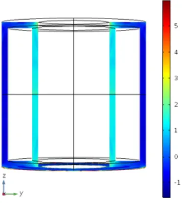
Figure 19: Magnetic field plots of the 10-ring model. From left to right, slices in theyz, xz, and xyplanes

of the orthogonal component of the field, all plots with the same scale measured in tesla. Theyz slice cuts

through coils and the xz slice cuts halfway between coils, so the latter field is weaker. This effect is visible

as a spreading of field lines in the left plot of Fig. 20. A close-up of the field defects in thexyslice is shown

in Fig. 21.

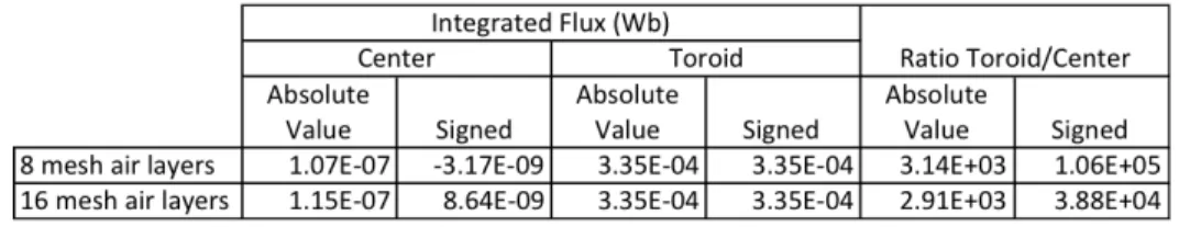
Table 1: Sample magnetic flux values for the 10-ring model with a normal-size mesh and 8 or 16 mesh layers

in the air sphere. Note that changing the mesh causes changes in the center flux. The center absolute values are higher than the signed values as expected and the toroid fluxes are unchanged.

the 10-ring model are shown in Fig. 19.

We expect that increasing the number of coils would improve the field directionality and homogeneity

and thus reduce the center field and increase the toroid field. For more coils the field lines of the left plot of

Fig. 20 would have less spillover outside the toroid region. We also expect the addition of G10 inside the coil

not to make much difference in the field, but this model has not yet been tested with the correct periodic

boundary conditions. A comparison of the fields from models with and without G10 with magnetic insulation

boundary conditions shows little change. The effect of the mesh on the field (Fig. 21 and Table 1) is not

insignificant, but is reduced for smaller mesh sizes. These numerical effects will be important to examine

more thoroughly in future simulations with noise sources to completely understand the effects of possible

Figure 20: Left, magnetic field lines in the 10-ring model with periodic boundary conditions on the slice

faces. Right, magnetic field lines in the 50-ring model (with G10) with magnetic insulation conditions on

the slice faces. The insulation in the 50-ring model prevents the field from correctly running azimuthally as 10-ring model. In both models, the streamlines were formed starting from points in the xy-plane. On the

left, the spacing between coils allows some of the magnetic field to spill out of the intended region. With

an increased number of coils and periodic conditions we expect the field lines to be approximately circular

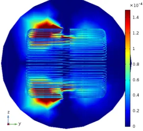
Figure 21: Comparison of mesh geometry and magnetic field defects, view over one coil slice from the +z

direction. Left, mesh elements in the xy-plane (color corresponds to mesh quality with red corresponding

to higher-quality elements). Right,z-component of the magnetic field in thexy-plane (color corresponds to

strength of the field with red corresponding to +z and blue to−z). Asterisks were placed at the corners of

4.3

Results

These studies offer a first examination of the magnet for the ABRACADABRA experiment. The primary

goal of the magnet construction is to reduce stray fields that could be a source of noise while maintaining the

strong field within the toroid that would source the axion effective current. The figure-of-merit that I used

to quantify this is the ratio of the central to toroid integrated magnetic flux. Here I explored two possible

designs, the continuously wound and multi-ring models. Although further testing is required, particularly of

the continuously wound version, the multi-ring model has the advantage of not having a built-in azimuthal

current sourcing a central field. In the multi-ring model, I tested various numbers of rings. The 10-ring

model exhibits fringing between the coils, so the eventual design would need to increase the number of rings.

The addition of G10 and changes to the current value were also tested inconclusively.

Moving forward, there are several numerical issues within COMSOL that need to be addressed. The

more complex models have issues with convergence. In addition to needing convergence in order to test

new designs, it would be useful to confirm that the models are converging to the correct field values.

Mesh-dependence of the solution is also a consideration that is addressed here and will need to continue to be

examined in the future. It appears that the mesh does affect the final value of the central field, but it will

important to check that these effects decrease for finer meshes. From here we will continue to explore these

and other aspects of the magnet design in order to reduce noise and allow ABRACADABRA be as sensitive

as it needs to be in order to search for cosmic axions.

5

Conclusions

ABRACADABRA has the potential to solve two important open questions in modern physics, the strong

CP problem and the mystery of dark matter. If it does not find axions, then it will have excluded a major

part of the axion phase space, the anthropic axion window. A positive signal would have impacts across

the globe, changing human understanding of our universe. In either case, ABRACADABRA will greatly

contribute to the knowledge of the physics community.

false signals. These magnet simulations will aid in the design of the prototype experiment, helping to ensure

that both it and the eventual full-scale experiment will be as sensitive as it needs to be to achieve the goal

theoretical limits.

References

[1] J.C. Kapteyn. First Attempt at a Theory of the Arrangement and Motion of the Sidereal System. ApJ,

55:302, may 1922.

[2] Teresa Marrod´an Undagoitia and Ludwig Rauch. Dark matter direct-detection experiments. J. Phys.,

G43(1):13001, 2016.

[3] Michael Klasen, Martin Pohl, and G¨unter Sigl. Indirect and direct search for dark matter. Prog. Part.

Nucl. Phys., 85:1–32, 2015.

[4] D S Akerib and Others. Results from a search for dark matter in the complete LUX exposure. 2016.

[5] C E Aalseth, P S Barbeau, J Colaresi, J I Collar, J Diaz Leon, J E Fast, N E Fields, T W Hossbach,

A Knecht, M S Kos, M G Marino, H S Miley, M L Miller, J L Orrell, and K M Yocum. CoGeNT:

A search for low-mass dark matter using p-type point contact germanium detectors. Phys. Rev. D,

88(1):12002, jul 2013.

[6] R. D. Peccei. QCD, Strong CP and Axions. (2):1–14, 1996.

[7] J M Pendlebury and Others. Revised experimental upper limit on the electric dipole moment of the

neutron. Phys. Rev., D92(9):92003, 2015.

[8] R D Peccei and Helen R Quinn. CP Conservation in the Presence of Pseudoparticles. Phys. Rev. Lett.,

38(25):1440–1443, jun 1977.

[9] Peter Svrcek and Edward Witten. Axions in string theory. Journal of High Energy Physics,

[10] Yonatan Kahn, Benjamin R Safdi, and Jesse Thaler. Broadband and Resonant Approaches to Axion

Dark Matter Detection. Phys. Rev. Lett., 117(14):141801, sep 2016.

[11] Andrei D Sakharov. Violation of CP invariance, C asymmetry, and baryon asymmetry of the universe.

Soviet Physics Uspekhi, 34(5):392, 1991.

[12] J. H. Christenson, J. W. Cronin, V. L. Fitch, and R. Turlay. Evidence for the 2πDecay of the K{2}ˆ{0}

Meson. Physical Review Letters, 13(4):138–140, 1964.

[13] Jonathan Engel, Michael J. Ramsey-Musolf, and U. Van Kolck. Electric dipole moments of nucleons,

nuclei, and atoms: The Standard Model and beyond.Progress in Particle and Nuclear Physics, 71:21–74,

2013.

[14] Alexandre Payez, Carmelo Evoli, Tobias Fischer, Maurizio Giannotti, Alessandro Mirizzi, and Andreas

Ringwald. Revisiting the SN1987A gamma-ray limit on ultralight axion-like particles. Journal of

Cosmology and Astroparticle Physics, 2015(02):006–006, 2015.

[15] Jihn E. Kim and Gianpaolo Carosi. Axions and the strong CP problem. Reviews of Modern Physics,

82(1):557–601, 2010.

[16] Leslie J Rosenberg. Dark-matter QCD-axion searches. InProc. Nat. Acad. Sci., 2015.

[17] Planck Collaboration. Planck 2015 results. XIII. Cosmological parameters. arXiv, page 1502.01589,

2015.

[18] COMSOL Multiphysics v. 5.2a.