Thesis.pdf

(1)

Electromagnet Design and Geometric Considerations for a

Positronium

CP

Violation Experiment

Ryan Petersburg

Senior Honors Thesis

Department of Physics and Astronomy

University of North Carolina at Chapel Hill

April 8, 2015

Abstract

Charge parity (CP) violation has not yet been definitively observed in the lepton sector. The

3-photon decay of orthopositronium has been used to search for such an asymmetry manifested

as a nonzero angular correlation ( ˆS·kˆ1)( ˆS·kˆ1×kˆ2) between the momentum vectors of the

three decay photons (|ˆk1| > |ˆk2| > |k~3|) and the orthopositronium spin ( ˆS). Current limits

on this correlation are at the 10−3 _{level. The} _CP _{Aberrant Leptons in Orthopositronium}

Experiment (CALIOPE) is attempting to improve this limit by reducing statistical uncertainties

with increased detector coverage. This thesis presents numerical studies to aid in the design of a

high-homogeneity electromagnet for use with CALIOPE. It also presents an experiment-specific

coordinate system to be considered for event geometry analysis.

(2)

1 Introduction

One of the most pressing issues in modern experimental particle physics and cosmology pertains

to the matter-antimatter asymmetry in the known universe. A requirement for this asymmetry is

charge parity (CP) violation as specified by the Sakharov conditions[13]. AlthoughCP violation has been observed in the quark sector through Kaon decay[6] and B-meson oscillations[1, 2], the

resulting CP violation is not enough to account for the disproportionate amount of matter and antimatter in the universe[11]. It is possible that some contribution to this asymmetry may come

from CP violation in the lepton sector, though this has not yet been observed despite studies with neutrinos[5] and the electron electric dipole moment[3]. Positronium could be another such

candidate, but previous experimentation has found no such asymmetry[9, 14] even to a sensitivity

of 2.2×10−3 [15]. CALIOPE (CP AberrantLeptons inOrthopositroniumExperiment) has been proposed by Dr. Reyco Henning and UNC graduate student Chelsea Bartram in order to improve

this limit.

This honors thesis begins by explaining the theoretical background of CP violation in Ps (Sec-tion 2) and then describing the experimental setup of CALIOPE to be used to more precisely

determine if such an asymmetry exists (Section 3). It then outlines the contributions of the author

to the experiment: optimization for an electromagnet (Section 4) designed around an established

detector array and development of a coordinate system (Section 5) based on the detector

configu-ration. All contributions by the author were presupposed to decrease systematic uncertainties in

the experiment resulting in the greatest possible precision.

2 CP

Violating Decay Process in Postronium

Positronium (Ps) is an unstable particle system composed of an electron and a positron. Ps can

exist in either the singlet (S = 0,ms= 0), parapositronium (p−P s), or triplet (S= 1,ms= 0,±1), orthopositronium (o−P s), quantum configuration depending on the relative spin orientations of the two bound fermions. When these two configurations are mixed, they can be distinguished

by the resulting number of gamma ray photons after decay (p−P s = even, o−P s = odd), which is inherently defined by Ps charge parity conservation. Though, the branching ratio for each

Ps configuration decay greatly favors the least possible number of resultant photons, meaning

(4)

to approximately 30 ns when Ps is placed in an external magnetic field (approximately 5 kG),

meaning the triplet ms=±1 states could be completely separated from all other states.

CP asymmetry in Ps would be manifested in the 3γ decay of o−P s with ms = ±1. If this decay ofo−P s isCP violating, there will exist a nonzero asymmetry functionA such that

A=CCPQ

withCP violation amplitudeCCP and unit-less angular correlation

Q= ( ˆS·ˆk1)( ˆS·ˆk1×kˆ2)

where ˆS is the normalized Ps spin orientation (S~) and ˆki are the normalized vectors of 3γ in order of decreasing momentum (|~k1|>|~k2|>|~k3|).

The asymmetry function A of the o−P s decay system is considered CP violating as follows. All of the five vectors that determineA change sign when undergoing time-reversal (T), therefore

AisT odd (i.e. T is asymmetric ifAis nonzero). The threeki vectors also change sign, unlike the axialS vector, when undergoing parity-reversal (P), therefore Ais also P odd. However, since the decay ofo−P sinto 3γ is defined as conserving charge parity, a charge-reversal (C) does not change

A’s sign, meaning A is C even. Combining these symmetry properties, A would be CP violating but not necessarily CP T violating ifCCP is observed to be nonzero.

A therefore denotes a small, possibly CP-violating, angular correlation that is superposed on the standard model predication for Ps decay, as computed by Bernreuther[4]. If CCP = 0, the angular distribution of 3γ will be identical to the Bernreuther distribution. But ifCCP is nonzero, there will be more events whereQ >0 and less events whereQ <0 than the number predicted by the Bernreuther distribution. More succinctly,

N( ˆS,kˆi) =NB( ˆS,kˆi)[1 +A( ˆS,ˆki)]

where N is the number of observed events with a certain ˆS and ˆki while NB is the Bernreuther

predicted number of events with the same set of ˆS and ˆki. If such a proportion (1 +A) is observed between these two distributions with A∝Q,CP violation ino−P s decay can be confirmed. The now calculableCCP =A/Qis predicted to be on the order of 10−10due to photon-photon final-state interactions[4]. This is, however, 7 orders of magnitude below current experimental limits.

3 The

CP

Aberrant Leptons in Orthopositronium Experiment

(5)

discrim-inating between the quantum states of a source of Ps, an external magnetic field that breaks the

spherical symmetry of the Ps system introducing a direction along which the spin vector (S~) can be defined, and a detector array to measure the coincident normalized momentum decay vectors

ˆ

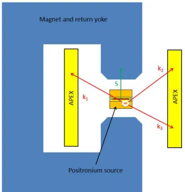
k1,ˆk2,kˆ3. These three requirements can all be fulfilled by CALIOPE which is shown in Figure 1

and further explained in the following sections. A Ps source (Section 3.2) is placed in a uniform

magnetic field created by an iron core electromagnet (Section 4) and the resultant 3γ are detected by a large angular acceptance array of scintillator detectors (Section 3.1).

Figure 1: Drawing of the CALIOPE experimental configuration, not to scale.

The primary goal for CALIOPE is to increase the number of event statistics and possibly

reduce systematic uncertainties from previous searches for CP violation in Ps which used the aforementioned experimental requirements. Previous experiments have been limited to analysis

of only a single decay plane for 3γ and an irreversible magnetic field with approximately 10% inhomogeneity. Through the CALIOPE experimental design, statistics (and therefore precision)

(6)

3.1 APEX Detector

The APEX detector (Figure 3), which was originally constructed for the ATLAS Positron

Ex-periment (APEX)[12], has been inherited by CALIOPE from the Laboratory for ExEx-perimental

Nuclear Astrophysics (LENA) and is currently housed at the Triangle Universities Nuclear

Labora-tory (TUNL) at Duke University. This detector is a cylindrical NaI(Tl) scintillator array segmented

into 24 position-sensitive bars around the circumference. A diagram of one of these bars in shown

in Figure 2, where the scintillating trapezoidal crystal has dimensions 55.0×6.0×5.5(7.0) cm3 (L ×W×H) and is surrounded by a 0.5 mm thick stainless steel container with a 4.4 cm×1.1 cm (D

× H) cylindrical quartz window on each end. Each NaI bar is ended with either two Hamamatsu

R580 or Photonis XP2012B photomultiplier tubes (PMTs) which could be magnetically shielded (a

combination of iron and mu-metal) within the PMT housing. Without the magnetic shield, these

PMTs would suffer a large gain reduction from even minimal (>1µT) longitudinal magnetic fields, as shown in Figure 4 for the Hamamatsu R580 PMTs. The NaI bars are attached to each other by

a stainless steel ring on each end, leaving an assembled detector array with 85.0 cm length, 56.7

cm outer diameter, 42.8 cm inner diameter, and 75% coverage of 4π from the geometric center[7].

(7)

Figure 3: Photograph by Stephen Daigle of the assembled APEX detector [7]

APEX will be used to determine the energy and directional components of the three ˆki photons by detecting the scintillation light of the photons interacting in the bars. The reconstructed position

along the length of the bar can be calculated as[7]

X= 1 2µln

A2

A1

(8)

Figure 4: Relative output for the Hamamatus R580, a 38 mm dia. head-on type PMT, based on

magnetic intensity both with and without shielding, taken from the manufacturer’s manual[10]].

The magnetic intensity is converted to the magnetic field in air byB =µ0H ⇒1 A/m = 4π×10−7T.

Figure 5: Schematic drawing of an NaI bar detailing the position reconstruction parameters [7]

3.2 Positronium Source

(9)

Chelsea Bartram. It will include a flat, foil-like positron source (22Na) surrounded by two layers

of cylindrical positron sensitive plastic scintillator connected to a set of PMTs by optical fiber.

These scintillators are surrounded by silica aerogel creating the cylindrical design shown in Figure

6 located at the geometric center of the APEX detector. When the positron is produced in the

source, it will pass through the plastic scintillator and set an initial timing signal to be sent by

optical fiber to the non-APEX PMTs. It will then enter the aerogel and combine with an electron

forming Ps. The Ps will migrate into the interstitial space and quickly decay into 3γ which will be subsequently detected by the APEX array and given a final time.

Figure 6: Cross-sectional drawing of the cylindrical positronium source with particle vectors, not

to scale

These two timing events are used to distinguish o−P s with ms = ±1 from p−P s and o−P s withms= 0. Those events that correspond to the 142 ns mean lifetime ofo−P sin the aerogel are kept while those that correspond to the 125 ps mean lifetime of p−P s and 30 ns mean lifetime of tripletms = 0 are rejected.

4 Electromagnet Design and Optimization

(10)

(5 kG = 0.5 T) magnetic field through the Ps source is necessary. The author’s contributions

to CALIOPE begin with the design of an electromagnet meant to accommodate for the APEX

detector and positronium source while providing such a reversible magnetic field. As detailed

in this section, the electromagnet was primarily optimized for magnetic homogeneity in the Ps

source and minimized longitudinal magnetic fields in the PMTs, while maintaining affordability

and feasibility. Throughout this section, the phrase “non-functional magnetic field” will be used

to describe the components of the magnetic field perpendicular to the “functional field” through

the Ps source which is parallel to the Ps spin orientation. All of the magnet simulation and data

analysis, including all simulated constructions and optimization plots in this section, was completed

using Radia[8], an electromagnet simulation package written for Mathematica.

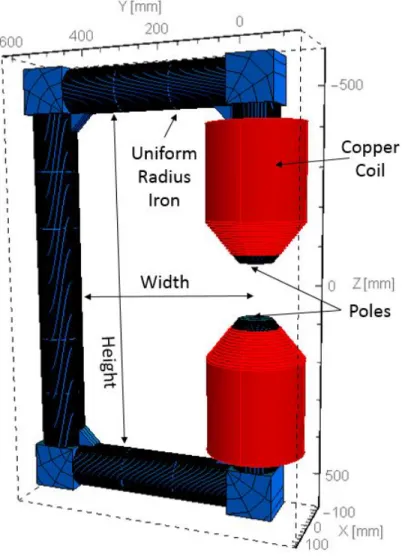
4.1 Finalized Design

The electromagnet design shown in Figure 7, where blue signifies the iron core and red signifies

the copper coils, is a highly optimized simulated construction. It has a height of 90.0 cm and a

width of 50.0 cm. The magnet’s return has a radius of 58 mm while the poles have a radius of

43 mm. This leaves a gap height of 141.5 mm and a pole chamfer height of 18.75 mm. The 5

mm diameter copper wire coils follows the angle of the magnet pole’s chamfer until the 13th layer,

where the remainder of the coil is uniformly cylindrical. The iron core, consisting of the purest iron

available (>99.9% purity), will weigh approximately 210 kg.

These parameters fulfill the geometric requirements of the Ps source and the APEX detector.

The magnet can provide a uniform magnetic field at the Ps source located at the center of the

detector array with minimized magnetic field strength at the PMTs. The magnet core’s return

will fit around the outside of the APEX detector, allowing for 360 degrees of rotation which can

be used to decrease azimuthal systematic uncertainty. Neither the iron core nor the copper coil

lies directly between the Ps source and any part of the NaI bars in the detector array, preventing

photon scattering or absorption before detection.

The general design scheme for this magnet was influenced by the magnet designs of two previous

Ps tests for CP violation[14, 15], one of which can be seen in Figure 24. The C-shape of these magnets could be easily adapted to the APEX detector geometry, therefore it was given initial

consideration. This basic design was then simulated in Radia, originally with a squared magnet

return that was eventually changed to cylindrical (more precisely, a 128-side prism, due to geometric

(11)

to decrease the required current by decreasing the coil distance to the Ps source position. The

squared corners shown in Figure 7 are artifacts of Radia and will be smoothed during manufacturing.

Figure 7: Simulated electromagnet construction

In order to increase simulation precision, all magnet simulations included 3-section lengthwise

voxelization for each segment of the magnet return, 5×5×5 voxelization for the magnet poles, and

3×3 corner voxelization for the four corners. For all magnetic field analysis and optimization studies,

the functional magnetic field at the center of the Ps source would be assumed to be 5.00±0.01 kG while the coil’s current iteratively converged to produce this field, thereby accommodating for

(12)

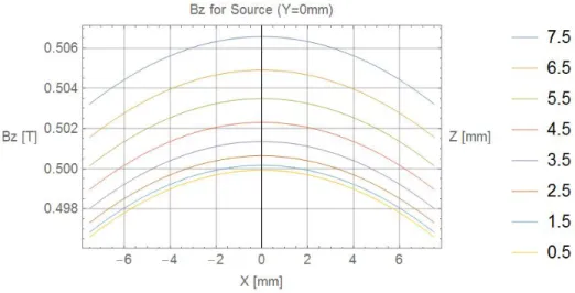
4.2 Magnetic Field at Ps Source

The plots shown in Figures 8, 9, and 10 detail the magnitude of the magnetic field’s three

components along the x-axis (defined in Figure 7) of the Ps source. Bz is defined as the functional field whileBx andBy are defined as non-functional fields. These plots show that the magnetic field throughout the Ps source is 98-99% homogenous, a large improvement from previous

experimen-tation [15]. The plot in Figure 11 further proves the directional uniformity of the magnetic field

between the magnet’s poles.

Figure 8: Simulated z-direction magnetic field throughout the xz-plane of the Ps source.

(13)

Figure 10: Simulated y-direction magnetic field throughout the xz-plane of the Ps source.

Figure 11: Simulated directional plot of magnetic field between the magnet poles. The color-coded

magnetic field magnitudes are in Tesla. The Ps source would be located at (0,0,0) with diameter

(14)

4.3 Magnetic Field at PMTs

As shown in Figure 4, the Hamamatsu R580 PMTs used in conjunction with the APEX detector

are restricted by the strength of longitudinal magnetic fields (> 1µT). Even with the standard magnetic shield cases provided by Hamamatsu that have a shielding factor of at most 103, these

PMTs would show significant gain reduction for magnetic fields greater than 10 G. Since the

optimization studies (Section 4.4) could not yield maximum PMT fields less than 100 G, a stronger

magnetic shield case made from a combination of iron and mu-metal or a fine-mesh PMT (e.g.

the Hamamatsu H8409-70) is highly recommended. A maximum PMT field strength of 300 G was

chosen for these optimization studies due to a test completed by the APEX experiment which found

only a 3% gain reduction in fine-mesh Hamamatsu R2490 PMTs coupled to the APEX detector

with a 300 G longitudinal field[12].

In Figures 12 and 13, the longitudinal field componentsBx andBy throughout the given PMT location (one of the locations with potentially maximum longitudinal fields) do not exceed 300 G,

meaning the PMTs should be usable with minimal gain reduction. The simulated directional plot

in Figure 14 gives a more complete understanding of the magnetic field directionality throughout

the experimental area.

(15)

Figure 13: Simulated y-direction magnetic field throughout the central yz-plane of a PMT.

Figure 14: Simulated directional magnetic fields throughout the yz-plane of the entire experimental

(16)

4.4 Optimization Considerations

As earlier introduced, the non-functional fields at the Ps source and in the PMTs need to be

minimized to achieve an optimized magnet design. An optimal magnet would have a non-functional

source field less than 2% relative to the functional source field and a longitudinal PMT field of less

than 300 G. Since this magnet will have a functional field of 5 kG, the longitudinal PMT field would

need to be less than 6% relative to the functional source field. However, these two fields tend to be

minimized at different ends of the range of magnet size parameters. Therefore, a weighted average

W is used between the non-functional relative source and PMT fields such that

W = 3·Source% +P M T% 4

where the constant 3 is used due to ratio between the maximum relative PMT field (6%) and

non-functional source field (2%). This weighted average has an error of approximately±0.05%. A minimized value (less than 2%) for the weighted average returns the optimal magnet parameters.

4.4.1 Height and Width

The color gradient plot shown in Figure 15 relating the height and width of the magnet design

reveals how the weighted average depends slightly on the magnet height and even less on the magnet

width. It also recommends a height just surrounding the PMTs. Therefore, the height of 90.0 cm

was definitively chosen, while the width of 50.0 cm was more arbitrarily chosen to be just outside

the large metal rings holding together the APEX detector.

Figure 15: Color gradient plot between the magnet’s height and width using a weighted average of

(17)

4.4.2 Radius and Pole Radius

The color gradient plots shown in Figure 16 and 17 give a very nice minima to the weighted

average optimization for the radius and pole radius of the magnet. They clearly recommend a

radius of 58±2 mm and a pole radius of 43±3 mm.

Figure 16: Color gradient plot between the magnet’s return radius and pole radius using a weighted

average of the relative non-functional source and longitudinal PMT magnetic fields.

Figure 17: A smaller range color gradient plot between the magnet’s return radius and pole radius

using a weighted average of the relative non-functional source and longitudinal PMT magnetic

(18)

4.4.3 Wire Diameter and Coil Size

The copper wire optimization included a greater number of tested parameters due to the limiting

nature of the copper wire’s ampacity and power dissipation which are listed in American Wire

Gauge (AWG) table in Figure 18. As seen in Figure 19, neither the wire diameter nor the number

of coil layers has a large effect on the weighted average, but the combination of both parameters

should not be too large to avoid crossing the 2% threshold. However, Figure 20 reveals that there

is a minimum number of coil layers before the current would have to exceed the wire’s ampacity

to produce the desired 5 kG magnetic field. The optimization is further hindered by the power

dissipation color gradient plot in Figure 21 which shows that larger wire diameter and greater

number of coils layers ultimately decrease the heat produced by the coil, yet the entire range of

parameters yielded greater than 1 kW.

Due to complexity of this optimization, a wire diameter of approximately 5 mm (AWG = 4)

and 13 coil layers is recommended and was used in these simulations studies, but further real world

testing should be completed to fully optimize these parameters. Addtionally, because the power

dissipation is expected to be greater than 1 kW, water-cooled copper wire coils will need to be

considered for future study.

Figure 18: Table of information regarding various copper wires based on the American Wire Gauge

(19)

Figure 19: Color gradient plot between wire diameter and number of coil layers using a weighted

average of the relative non-functional source and longitudinal PMT magnetic fields.

Figure 20: Color gradient plot between wire diameter and number of coil layers using the wire’s

current.

Figure 21: Color gradient plot between wire diameter and number of coil layers using the coil’s

(20)

4.5 Failed Designs

Figure 22: Failed magnet designs with a) ends thicker than the return, b) return thicker than the

ends, and c) no return

The three designs in Figure 22 were all previously tested and optimized to see if they showed

any significant improvement over the given finalized design. Changing the magnet’s return radius

relative to the end radius as seen in Figure 22a and b, provided a very slight (<0.1%) improvement in the relative field weighted average when the return was 5-10 mm larger than the end, but this

was not justified due to the significantly higher complexity of manufacturing such an iron core. The

return was also removed completely as seen in 22c, but this drastically increased the non-functional

magnetic field at the PMTs and would be unrealistically unsafe for the magnet’s operators due to

the unshielded magnetic field produced outside the detector array.

5 Geometrical Considerations

As explained in Section 2, the experimental asymmetry function A depends on the vectors ˆS

and ˆki which must be defined by a set of generalized parameters. These parameters are typically related to the coordinate system in which the event analysis takes place. This section describes a

(21)

altered set of parameters optimized for use in CALIOPE.

5.1 Yamazaki Coordinate System

In the Yamazaki positroniumCP violation experiment[15], they define the angular correlation Q as

Q(θ, ψ, φ) = ( ˆS·ˆk1)( ˆS·ˆk1×ˆk2) =P2sin 2θsinψcosφ,

where θ is the angle between ˆS and N~ = ˆk1×kˆ2, ψ is the angle between ˆk1 and ˆk2, and φis the

angle between ˆk1 and the projection of ˆS onto the plane defined byN~. These angles can be seen in

Figure 23. This system works well considering the experimental setup shown in Figure 24 used by

the Yamazaki group. They were able to control both θ and ψ: using the turntable at a set angle (30◦) relative to the magnetic field to defineθand having pairs of LYSO scintillator detectors with set angles (150◦) on this turntable to define ψ. Therefore, the Yamazaki group was able to define the asymmetry in Ps using only the cosφterm inQmeaningQ=Q(φ) andA=A(φ) =CCPQ(φ). Experimentally, they determinedA through a derivation beginning with the formula described in Section 2:

N(φ) =NB(φ)[1 +A(φ)]⇒N(φ+ 180◦) =NB(φ+ 180◦)[1 +A(φ+ 180◦)]

NB(φ) =NB(φ+ 180◦)⇒

N(φ) 1 +A(φ) =

N(φ+ 180◦) 1 +A(φ+ 180◦)

A(φ) =−A(φ+ 180◦)⇒N(φ)[1−A(φ)] =N(φ+ 180◦)[1 +A(φ)]

N(φ)−N(φ+ 180◦) =A(φ)[N(φ) +N(φ+ 180◦)]

where theNBequivalence exists becauseNB(ˆk1,ˆk2,kˆ3) =NB(−kˆ1,−ˆk2,−ˆk3)[4]. Thus, by counting

the number of 3γ events defined by ˆk1 hitting the detector at a determined angleφand at the exact

opposite angle φ+ 180◦, they could calculate the asymmetry term

A(φ) =CCPQ(φ) =

N(φ)−N(φ+ 180◦)

N(φ) +N(φ+ 180◦₎

which varies along only one dimension as seen in their asymmetry plot Figure 25. Their result was

(22)

Figure 23: Representation of the Yamazaki coordinate system for a single decay event

(23)

Figure 25: Asymmetry results for the Yamazaki positronium CP violation experiment. The line depicts an angular correlationA withCCP = 0.01

5.2 CALIOPE Cylindrical Geometry

Figure 26: Representation of the CALIOPE coordinate system for a single decay event

The experimental setup for CALIOPE, however, is very different from that used with the

Yamazaki experiment. CALIOPE uses a cylindrical detector made from scintillator bars that

(24)

pertaining to the 3γ events is a combination of a calculated X position using the weighted signals from two PMTs and an approximate azimuthal angle to within 15◦. From these values, CALIOPE

could reconstruct ˆk1 and ˆk2 and calculate the angular correlation Q(θ, ψ, φ) using the Yamazaki

coordinate system. However, there would be significant error correlations during these calculations,

leading to harder-to-quantify systematic uncertainties: θmust account for error with both ˆk1 and

ˆ

k2 due to theN~ calculation,ψmust also account for error with both ˆk1 and ˆk2, andφaccounts for

error with ˆk1 and again for ˆk1 and ˆk2 due to theN~ calculation.

Instead, the author suggests CALIOPE use a cylindrical coordinate system to better match

the experimental detector geometry. The z-axis is defined as the length axis of APEX and the

azimuthal angle is defined around its circumference. Using these cylindrical coordinates, (ρ, φ, z), the spin and 3γ vectors can be defined as

~

S = (0,0, zS), Sˆ= (0,0, zS,norm)

~_k_i_{= (}_r_i_{, δ}_i_{, z}_i₎_, _kˆ_i_{= (}_r_i,_norm_{, δ}_i,_norm_{, z}_i,_norm₎ where ri, δi, and zi are shown in Figure 26; ri,norm = _|_~r_ki

i|

, δi,norm = δi, and zi,norm = _|_~_kzi

i|

are the

normalized cylindrical components that define ˆki; and zS,norm = ±1 since the Ps spin orientation

is defined as parallel to the z-axis. The two coordinates ri,norm and zi,norm can be calculated using

the experimental quantities found in Figure 26 as

ri,norm=

R

q

R2₊_z2

i

= sinαi

zi,norm =

zi

q

R2₊_z2

i

= cosαi

where R is the average radius of the APEX detector,zi=Xdefined in Section 3.1 as the longitudinal position in the NaI bar for the respective photon, and αi are the angles between ˆki and the plane defined by the z-axis as the normal (−180◦< αi <180◦). The anglesαi are included to help show howri,norm and zi,norm are limited quantities. Now the angular correlationQcan be derived:

( ˆS·ˆk1) =zS,normz1,norm

( ˆS·ˆk1×kˆ2) =zS,normr1,normr2,norm(cosδ1sinδ2−sinδ1cosδ2) =zS,normr1,normr2,normsin (δ2−δ1)

(25)

whereδ =δ2−δ1 the azimuthal angle between ˆk1 and ˆk2. Converting Qto measurable quantities,

Q(z1, z2, δ) =

Rz1

R2₊_z2 1

R

p

R2₊_z2 2

sinδ= 1

2sin 2α1cosα2sinδ

Therefore, the calculation of the asymmetryAis dependent on four parameters, z1,z2,δ1, and,δ2,

which are all directly measured by the APEX detector. Using the inherent identitiesNB(z1, z2, δ1, δ2) =

NB(−z1,−z2, δ1+ 180◦, δ2+ 180◦) andA(z1, z2, δ1, δ2) =−A(−z1,−z2, δ1+ 180◦, δ2+ 180◦),Acan

be experimentally derived to be

A(z1, z2, δ1, δ2) =CCPQ(z1, z2, δ1, δ2) =

N(z1, z2, δ1, δ2)−N(−z1,−z2, δ1+ 180◦, δ2+ 180◦)

N(z1, z2, δ1, δ2) +N(−z1,−z2, δ1+ 180◦, δ2+ 180◦)

6 Conclusions

The CP Aberrant Leptons in Orthopositronium Experiment is attempting to decrease the currently established limits on the CP violation parameter CCP for the 3γ decay of o−P s. The project is set to minimize the statistical uncertainties from previous o−P s CP violation searches (2.2×10−3) using the APEX detector with large angular acceptance, and a reversible magnetic field. The electromagnet presented in this thesis was optimized to reduce non-functional magnetic

fields at the Ps source and detector PMTs. This was accomplished with 98-99% homogeneity

at the Ps source and a less than 300 G longitudinal magnetic field at the PMTs, well within

heavily shielded or fine-mesh PMT limitations. An event analysis geometry unique to CALIOPE

was also introduced in order to reduce propagation of error in the asymmetry calculation. If this

electromagnet, detector, and coordinate system are used for the CALIOPE runs, set for Fall 2015,

the measurements of CP asymmetries in the 3γ decay of o−P s will have improved systematic uncertainties.

7 Acknowledgments

This project was supported by the Gillian T. Cell Senior Thesis Research Award in the College of

Arts & Sciences, administered by Honors Carolina. This material is based upon work supported by

the U.S. Department of Energy, Office of Science, Office of Nuclear Physics under Award Numbers

DE-FG02-97ER41041 and DE-FG02-97ER41033. Special thanks is due to my advisor Dr. Reyco

Henning and UNC graduate student Chelsea Bartram for their support throughout the entire

(26)

feasibility of the unique electromagnet design. This document was written to fulfill the requirements

of the senior honors thesis at the University of North Carolina at Chapel Hill.

References

[1] A. Abashian et al. Measurement of the CP violation parameter sin 2φ1 in Bd0 meson decays.

Phys.Rev.Lett., 86:2509–2514, 2001.

[2] B. Aubert et al. Measurement of CP violating asymmetries in B0 decays to CP eigenstates.

Phys.Rev.Lett., 86:2515–2522, 2001.

[3] J. Baron et al. Order of Magnitude Smaller Limit on the Electric Dipole Moment of the

Electron. Science, 343:269–272, 2014.

[4] W. Bernreuther and O. Nachtmann. Weak Interaction Effects in Positronium. Z.Phys., C11:235, 1981.

[5] J. Burguet-Castell, M. Gavela, J. Gomez-Cadenas, P. Hernandez, and O. Mena. Superbeams

plus neutrino factory: The Golden path to leptonic CP violation. Nucl.Phys., B646:301–320,

2002.

[6] J. Christenson, J. Cronin, V. Fitch, and R. Turlay. Evidence for the 2 pi Decay of the k(2)0

Meson. Phys.Rev.Lett., 13:138–140, 1964.

[7] S. Daigle. Low Energy Proton Capture Study of the 14N(p, γ)15O Reaction. PhD thesis, University of North Carolina at Chapel Hill, 2013.

[8] European Synchrotron Radiation Facility, http://www.esrf.eu/Accelerators/Groups/

InsertionDevices/Software/Radia. Radia.

[9] M. Felcini. A Test of CP symmetry in positronium. Int.J.Mod.Phys., A19:3853–3864, 2004.

[10] Hamamatsu Photonics, https://www.hamamatsu.com/resources/pdf/etd/PMT_handbook_

v3aE.pdf. Photomultiplier Tubes: Basics and Applications, 3a edition, 2007.

[11] C. Jarlskog. A Basis Independent Formulation of the Connection Between Quark Mass

(27)

[12] N. Kaloskamis, K. Chan, A. Chishti, J. Greenberg, C. Lister, et al. The Trigger detector for

APEX: An Array of position sensitive NaI(Tl) detectors for the imaging of positrons from

heavy ion collisions. Nucl.Instrum.Meth., A330:447–457, 1993.

[13] A. Sakharov. Violation of CP Invariance, c Asymmetry, and Baryon Asymmetry of the

Uni-verse. Pisma Zh.Eksp.Teor.Fiz., 5:32–35, 1967.

[14] M. Skalsey and J. Van House. First test of CP invariance in the decay of positronium.

Phys.Rev.Lett., 67:1993–1996, 1991.

[15] T. Yamazaki, T. Namba, S. Asai, and T. Kobayashi. Search for CP-violation in Positronium

Thesis.pdf

Electromagnet Design and Geometric Considerations for a

Positronium

CP

Violation Experiment

Contents

1

Introduction

2

CP

Violating Decay Process in Postronium

3

The

CP

Aberrant Leptons in Orthopositronium Experiment

4

Electromagnet Design and Optimization

5

Geometrical Considerations

6

Conclusions

7

Acknowledgments

References