216
A new combination of multi-mode resource-constrained
project scheduling and group decision-making process
with interval-fuzzy information
M. Ghasemi
1, S.M. Mousavi
1*, S. Aramesh
11 Department of Industrial Engineering, Shahed University, Tehran, Iran
[email protected], [email protected], [email protected]
Abstract
Multi-mode resource-constrained project scheduling problem (MRCPSP) is one of the most important extensions of the basic RCPSP. In this paper, a new mathematical model for MRCPSP is presented with a time-quality trade-off approach. The model has two objectives, the first objective minimizes the project completion time, and the second objective maximizes the project quality while the quality of activities can be increased based on the reworking. In addition, in the presented model, total available resources, including renewable and non-renewable, are decision variables. The quality and duration of project activities are interval forms. For this purpose, a new expert weighting method based on interval information is presented to unify the experts’ views. The group decision-making method applies a bi-directional projection measure to the positive ideal solution and two negative ideal solutions. Moreover, a new extended interval-fuzzy solution method based on goal programming is proposed to deal with the interval information and mathematical model objectives. The presented mathematical model and group decision-making method are solved with a dataset, and some sensitivity analyses are reported. Keywords: MRCPSP, group decision-making method, bi-directional projection measure, interval information, reworks
1-Introduction
People often encounter huge decision-making challenges with respect to the field of scientific management, engineering disciplines, and our daily life (Tian et al., 2016; Peng and Liu, 2017; Zavadskas et al., 2017; Deli, 2015; Birjandi et al., 2019). Group decision-making (GDM) is defined as the act of making decisions by a group of decision-makers (DMs) faced by a decision-making problem. GDM is necessary due to increasing complexity in many real decision situations (Baudry et al., 2018; Yue, 2018). Nowadays, the GDM has been transformed into a universal and essential attribute in human communities. In fact, GDM is now considered as an inseparable component of modern decision and operational studies (e.g., Dorfeshan et al., 2019, 2020; Moghiseh et al., 2019; Mohagheghi et al., 2019a,b; Haghighi et al., 2019).
*Corresponding author
ISSN: 1735-8272, Copyright c 2020 JISE. All rights reserved
Journal of Industrial and Systems Engineering Vol. 13, No. 1, pp.216-239
217
The DMs are usually specialized in various academic disciplines. Therefore, each DM owns distinctive attributes, with respect to knowledge, skills, experience, and personality. That is why each DM usually has contrasting attitudes and inconsistent impacts on overall decision results, i.e., each DM influences on the outcome asymmetrically. Hence, the various ways in which weights of DMs are measured are promising and important research topics which have been receiving more and more attention. The nature of the problem, context, and authenticity of DMs are among primary influential factors on the quality of the decision-making processes in the problem area (Wang et al., 2013). As increasing in the complexity of socio-economic environment, it becomes harder for a DM to confront all the respective features of an obstacle (Dey et al., 2017). Many decision-making obstacles must arise in a group environment with respect to the real world. More complications will emerge in the analysis by moving from a DM to multiple DMs. As a result, approaches associated with group decision-making (GDM) problems have been recently in the center of convergence among scholars (Yang and Du, 2015; Hancerliogullari et al., 2017; Liao et al., 2017).
Among existing GDM approaches, projection measure has been advantageous in terms of taking both the distance and the included angle among evaluated alternatives. TOPSIS, as a pretty straightforward MCDA method, is an acronym that represents technique for order preference by similarity to ideal solution (Chen, 2015; Hwang and Yoon, 1981). TOPSIS is a standard methodology in decision science and GDM solutions, in which the positive and negative ideal decision(s) are designated (Yue, 2014; 2017). The Euclidean and Hamming distances are the most common measures (Das and Kar, 2014). In essence, the projection measure (Tsao and Chen, 2016; Yue, 2014; 2015; 2017), as a more comprehensive consideration for measuring the separation, highlights the angle between two decision objectives. The projection measure in decision science is implemented when a vector/matrix is close to another (Tsao and Chen, 2016; Yue and Jia, 2015). Projection methods have been greatly investigated by researchers (Zhang et al., 2013) and effectively employed to many multi-attribute decision-making (MADM) problems (Chen, 2016). To illustrate, two projection models in uncertain MADM context and a projection-based compromising method for MADM with interval-valued intuitionistic fuzzy information were suggested by Xu and Da (2004) and Tsao and Chen (2016), respectively. In addition, Xu and Hu (2010) and Wang et al. (2012) explored projection model-based strategies to MADM with intuitionistic fuzzy information. The subjects of GDM are mainly complicated, questionable, and constrained to experts’ knowledge and personal impression. It is sometimes challenging to quantify the corresponding features. Accordingly, their values should be considered as intervals (Yue, 2012). For instance, Liu (2017) proposed two GDM methods based on interval-valued intuitionistic fuzzy power Heronian aggregation operators. Besides, Yue (2016) simulated a geometric approach to categorize interval-valued intuitionistic fuzzy numbers (IVIFNs) which were applied to GDM problems. Liu et al. 2018 solved the GDM problem with the interval information in the weight of attributes. Nguyen (2016) also introduced a new interval-valued knowledge measure for interval-valued intuitionistic fuzzy sets and implementing in GDM. Determining the weight of the DMs where the individual decisions are interval is presented by Yang et al. (2018). Besides, Liu (2016) used the VIKOR to solve the GDM problem where the numbers are interval. Interval numbers are suitable for the papers with the hybrid information (Yue, 2018) or heterogeneous GDM problems (Yu et al., 2018). In most of the GDM with the interval information, the positive ideal solution is considered. But in Yue (2019) the positive ideal solution and two negative ideal solutions are used to evaluate the normalized projection of individual decisions. In this paper, bidirectional projection is used to measure the relative closeness to the individual decisions.
Project scheduling problem (PSP), as one of the most essential constituents in project management, guarantees the success of the project in terms of project final cost and makespan (Birjandi and Mousavi, 2019a). Boosting the project scheduling is considered as a delicate task owing to its required activities and demanding resources. Recently, implementation of the project scheduling has been intensified in some industry sectors, such as engineering, production, maintenance, and construction. Fulfilling the activities’ preference and assigning the adequate resources would usually result from scheduling with finite resources. The estimated and expected times for each activity’s employment during the planning
218
phase are not often matched. Nevertheless, it is crucially important to specify a time for implementation of each activity in the project management since it is advantageous for the makespan (Turner et al., 1999). Minimizing the total project duration or makespan as a result of scheduling activities’ goals to resource and technological impediments is the standard problem in the context of project scheduling (Wuliang and Chengen, 2009). This is also known as the resource-constrained project scheduling problem (RCPSP). RCPSP and its extended versions have been studied since the 1960s and considered as one of the most broadly-studied scheduling problems (Muritiba et al., 2018). Precedence- and resource-feasible schedule have been introduced as a solution to the RCPSP, in which the makespan of a project is extensively shortened. RCPSP’s fundamental assumption states that continuous activities are non-preemptable. The idea of multi-mode resource-constrained project scheduling problem (MRCPSP) is one of the well-studied RCPSP-derived concepts. In fact, MRCPSP implies that activities are able to be accomplished in various execution modes (i.e., duration and resource requirements combinations). A single mode per activity is chosen, and the project makespan is minimized subject to precedence relations and (non)renewable resource limitations. Minimum makespan must include a list of all activities in the MRCPSP. In addition, the limitations of activities precedence, non-renewable resource consumption, and allocation of renewable resources need to be considered in minimum makespan (Muritiba et al., 2018). For more information on the MRCPSP, please see Weglarz et al. (2011).
The goal for more than 90% of project managers is maximizing projects’ characteristic and their results. Consistency between a project's outcome and customer's requirements is evaluated by project managers to validate projects’ qualifications. They also measure to what extend the project completes within the defined budget and on schedule. To achieve the latter goal, project managers attempt to remove the modification with respect to poorly accomplished activities. In the traditional RCPSP formulations, on the other hand, the overall assumption claims that work will be finished as scheduled and that modification won’t be necessary. Nevertheless, this assumption is not distinctly coherent, considering many modern projects. Project managers reported (Icmeli-Tukel and Rom, 1997) at least one inconsistent activity in their implemented projects which should be modified. Although modifications or reworking as it is widely known is one of the important issues in project scheduling, there are still limited studies associated with it. These studies are required, especially when outcomes of an activity deviate from its presupposed qualifications, non-comparative cases, or defect (Arditi and Pattanakitchamroon, 2006). The effect of rework on schedule delays was investigated by Hegazy et al. (2011). They also suggested following an optimized strategy to support decisions on cost-effective corrective action strategy. In addition, Hwang et al. (2009) evaluated the impact of rework on construction cost performance for a broad spectrum of projects.
Overlapping-oriented quality problems are removed by implementing modifications to correct design flaws emerging from incomplete data. Previous studies have accounted for quality as an essential agent in trade-off problems, stating that overall project quality achieved by project activities should be maximized within the required deadline and budget. Implementing a continuous scale from zero to one to determine the quality of each activity has also been elevated by such studies (Babu and Suresh, 1996; Tareghian and Taheri, 2006). Correlation between time, cost, and quality objectives calculated by a set of functions exist in the continuous trade-off problems. By the time research attempts to progress in the field and practical needs arise, researchers start focusing on the enhancement of methodologies to resolve the segregated time-cost trade-off problems (DTCTPs) (Hazır et al., 2011; Sonmez and Bettemir, 2012; Wuliang and Chengen, 2009; Xu et al., 2012). Generally, a decrease either in time or cost, on the other hand, declines the project quality (Cheng et al., 2016).
In this paper, a new decision-making method is presented. The presented GDM method is developed based on the bidirectional projection measure. Projection-based methods in the deterministic environment, and the uncertainties are essential parts of any project, so in this paper, the extended projection-based GDM is presented using interval numbers, where the duration and quality of activities are interval. These parameters are determined by extended GDM method by considering positive ideal solution and two negative ideal solutions. In addition, a new MRCPSP model with time-quality trade-off is proposed. In the mathematical model, the quality of activities can be increased by reworking. The
219
presented model is solved with a new extended interval-fuzzy solution method. The combination of decision-making method and mathematical model with interval information is a new context that this paper has brought up.
The rest of the study is organized as follows: in section 2, some preliminary definitions are defined. Next, section 3 describes the decision-making procedure. In section 4, the problem definition is proposed. After that the result of the solved model is presented in section 5. Then, sensitivity analyses are presented in section 6. Finally, the concluding is proposed in section 7.
2-Preliminary
In this section, some basic definitions regarding bidirectional projection between interval numbers which are useful in this paper are provided.
Definition 1. Let 𝑎 = [𝑎𝑙, 𝑎𝑢] = {𝑥|𝑎𝑙≤ 𝑥 ≤ 𝑎𝑢}, then 𝑎 is known as an interval number. In addition, 𝑎 is a positive interval number if 0 ≤ 𝑎𝑙 ≤ 𝑥 ≤ 𝑎𝑢, and the 𝑎 is a real number if 𝑎𝑙 = 𝑎𝑢.
Definition 2. Let 𝑎 = {[𝑎1𝑙, 𝑎1𝑢], … , [𝑎𝑛𝑙, 𝑎𝑛𝑢]} and 𝑏 = {[𝑏1𝑙, 𝑏1𝑢], … , [𝑏𝑛𝑙, 𝑏𝑛𝑢]} be two interval vectors, then 1. ‖𝑎‖ = √∑𝑛𝑗=1[(𝑎𝑗𝑙)2+ (𝑎𝑗𝑢)2] and ‖𝑏‖ = √∑𝑛𝑗=1[(𝑏𝑗𝑙)2+ (𝑏𝑗𝑢)2] are the module of 𝑎 and 𝑏. 2. 𝑎. 𝑏 = ∑𝑛𝑗=1(𝑎𝑗𝑙𝑏𝑗𝑙+ 𝑎𝑗𝑢𝑏𝑗𝑢) is the inner product between 𝑎 and 𝑏.
3. cos(𝑎, 𝑏) =‖𝑎‖ ‖𝑏‖𝑎.𝑏 is called the cosine of the included angle between 𝑎 and 𝑏. 4. The projection of vector 𝑎 on the vector 𝑏 is 𝑃𝑟𝑜𝑗𝑏(𝑎) = ||𝑎|| cos(𝑎, 𝑏).
Definition 3. Let 𝑎 = {[𝑎1𝑙, 𝑎1𝑢], … , [𝑎𝑛𝑙, 𝑎𝑛𝑢]} and 𝑏 = {[𝑏1𝑙, 𝑏1𝑢], … , [𝑏𝑛𝑙, 𝑏𝑛𝑢]} be two interval vectors,then the bidirectional projection is obtained as follows:
𝐵𝑃𝑟𝑜𝑗𝑏(𝑎) = 1 1+|𝑎.𝑏 ||𝑎||−
𝑎.𝑏 ||𝑏|||
=‖𝑎‖‖𝑏‖+|‖𝑎‖−‖𝑏‖|𝑎.𝑏‖𝑎‖‖𝑏‖ , (1)
Where 𝑎. 𝑏 is the inner product, and ‖𝑏‖ and ‖𝑎‖ are the modules of 𝑎 and 𝑏.
3-Decision making method
In this section, an extended method for the multiple criteria group decision-making problems with the interval information by using the bidirectional projection based on Yue (2019) is presented. In the multiple attribute group decision-making problems with the interval information, let 𝐴 = {𝐴1, 𝐴2, . . . , 𝐴𝑚} be a set of alternatives, 𝐶 = {𝐶1, 𝐶2, . . . , 𝐶𝑛} be the set of criteria, and 𝐷 = {𝐷1, 𝐷2, . . . , 𝐷𝑡} be the set of DMs. The DM k (𝑘 = {1,2, … , 𝑡}) provide the evaluation of criteria J (𝐽 = {1,2, … , 𝑛}) for the alternative I (𝐼 = {1,2, … 𝑚}) by using the interval date which is shown as 𝑥𝑖𝑗𝑘 = [𝑥𝑖𝑗𝑘𝑙,𝑥𝑖𝑗𝑘𝑢]. Thus the decision matrix with the interval numbers for the 𝑘𝑡ℎ DM is called 𝑋̅
𝑘 and established as follows:
𝑋̅𝑘 = (𝑥̅𝑖𝑗𝑘)𝑚×𝑛 = [
[𝑥11𝑘𝑙, 𝑥11𝑘𝑢] [𝑥12𝑘𝑙, 𝑥12𝑘𝑢] … [𝑥1𝑛𝑘𝑙, 𝑥1𝑛𝑘𝑢] [𝑥21𝑘𝑙, 𝑥21𝑘𝑢]
⋮ [𝑥𝑚1𝑘𝑙 , 𝑥𝑚1𝑘𝑢]
[𝑥22𝑘𝑙, 𝑥22𝑘𝑢] … ⋮ [𝑥𝑚2𝑘𝑙 , 𝑥𝑚2𝑘𝑢] …
[𝑥2𝑛𝑘𝑙, 𝑥2𝑛𝑘𝑢] ⋮ [𝑥𝑚𝑛𝑘𝑙 , 𝑥𝑚𝑛𝑘𝑢]]
220
The weight vector of criteria which is obtained by 𝑘𝑡ℎ DM is (𝑤
1𝑘, 𝑤2𝑘, … , 𝑤𝑛𝑘)𝑇 with 𝑤𝑗≥ 0 and ∑ 𝑤𝑗 𝑗 = 1.
The normalized decision matrix is dependent on the effect of the criterion on the problem, so the decision for the benefit criteria is normalized based on:
{
𝑟𝑖𝑗𝑘𝑙 = 𝑥𝑖𝑗 𝑘𝑙 √∑𝑚 (𝑥𝑖𝑗𝑘𝑢)2
𝑖=1
,
𝑟𝑖𝑗𝑘𝑢= 𝑥𝑖𝑗 𝑘𝑢 √∑𝑚 (𝑥𝑖𝑗𝑘𝑙)2
𝑖=1
,
(3)
And for the cost criteria the decision is normalized by using
{ 𝑟𝑖𝑗𝑘𝑙 =
1 𝑥𝑖𝑗𝑘𝑢 ⁄
√∑ (1 𝑥𝑖𝑗𝑘𝑙 ⁄ )
2 𝑚
𝑖=1
.
𝑟𝑖𝑗𝑘𝑢= 1
𝑥𝑖𝑗𝑘𝑙 ⁄
√∑ (1 𝑥𝑖𝑗𝑘𝑢 ⁄ )
2 𝑚
𝑖=1
.
. (4)
The normalized decision matrix is converted to the weighted decision matrix as follows:
𝑌̅𝑘 = (𝑤𝑗𝑘𝑟̅𝑖𝑗𝑘) = (𝑤j𝑘𝑟𝑖𝑗𝑘). (5)
To determine the weight of DMs, the positive ideal decision (PID) is considered as follows:
𝑌̅∗= (𝑦
𝑖𝑗∗𝑙, 𝑦𝑖𝑗∗𝑢)𝑚×𝑛, (6)
Where 𝑦𝑖𝑗∗𝑙 =1
𝑡∑ 𝑦𝑖𝑗 𝑘𝑙 𝑡
𝑘=1 and 𝑦𝑖𝑗∗𝑢 = 1
𝑡∑ 𝑦𝑖𝑗 𝑘𝑢 𝑡
𝑘=1 .
In this paper, two negative ideal decision (NID) are considered. First of all, the minimum decision is obtained as follows:
𝑌̅𝑙 = (𝑦𝑖𝑗−𝑙, 𝑦𝑖𝑗−𝑢)𝑚×𝑛, (7)
Where 𝑦𝑖𝑗−𝑙 = min𝑘∈𝑇𝑦𝑖𝑗𝑘𝑙 and 𝑦𝑖𝑗−𝑢 = min𝑘∈𝑇𝑦𝑖𝑗𝑘𝑢.
Similarly, the maximum decision is another NID which is determined as follows:
𝑌̅𝐶 = (𝑦𝑖𝑗+𝑙, 𝑦𝑖𝑗+𝑢)𝑚×𝑛, (8)
Where 𝑦𝑖𝑗+𝑙 = max𝑘∈𝑇 𝑦𝑖𝑗𝑘𝑙 and 𝑦𝑖𝑗+𝑢= max𝑘∈𝑇𝑦𝑖𝑗𝑘𝑢.
221 𝐵𝑃𝑟𝑜𝑗(𝑌̅∗, 𝑌̅𝑘) =
‖𝑌̅∗‖‖𝑌̅ 𝑘‖ ‖𝑌̅∗‖‖𝑌̅
𝑘‖ + |‖𝑌̅𝑘‖ − ‖𝑌̅∗‖|𝑌̅∗. 𝑌̅𝑘
. (9)
𝐵𝑃𝑟𝑜𝑗(𝑌̅𝑙, 𝑌̅𝑘) =
‖𝑌̅𝑙‖‖𝑌̅𝑘‖
‖𝑌̅𝑙‖‖𝑌̅𝑘‖ + |‖𝑌̅𝑘‖ − ‖𝑌̅𝑙‖|𝑌̅𝑙. 𝑌̅𝑘
. (10)
𝐵𝑃𝑟𝑜𝑗(𝑌̅𝐶, 𝑌̅𝑘) =
‖𝑌̅𝐶‖‖𝑌̅𝑘‖
‖𝑌̅𝐶‖‖𝑌̅𝑘‖ + |‖𝑌̅𝑘‖ − ‖𝑌̅𝐶‖|𝑌̅𝐶. 𝑌̅𝑘
. (11)
An extended relative closeness is evaluated as follows:
𝑁𝑅𝐶
𝑘=
𝐵𝑃𝑟𝑜𝑗(
𝑌̅
∗ , 𝑌
̅
𝑘)
𝐵𝑃𝑟𝑜𝑗
(
𝑌̅
∗, 𝑌̅
𝑘)
+ 𝐵𝑃𝑟𝑜𝑗(
𝑌̅
𝑙, 𝑌̅
𝑘)
+ 𝐵𝑃𝑟𝑜𝑗(
𝑌̅
𝐶, 𝑌̅
𝑘)
(12)
Each expert’s weight is calculated based on:
𝜆𝑘=
𝑁𝑅𝐶
𝑘∑𝑘
𝑁𝑅𝐶
𝑘. (13)
The weight of DMs is used to build the decision matrix as follows:
𝑌 = ∑𝑇𝑘=1𝜆𝑘𝑌̅𝑘. (14)
To sum up, the procedure of an extended decision-making method is described as follows:
Step 1. For the interval information, the decision matrix is constructed as shown by equation (2). Step 2. The individual decisions are normalized based on equations (3)-(4).
Step 3. The weighted normalized decision is evaluated based on equation (5).
Step 4. The positive ideal decision and two negative ideal decisions are formed by equations (6)-(8).
Step 5. The bidirectional projection measurement for individual decisions is calculated based on equations (9) - (11).
Step 6. The relative closeness of each DM is evaluated by equation (12). Step 7. The DM’s weight is calculated based on equation (13).
Step 8. The aggregated decision is constructed by equation (14).
4- Problem definition
The classic MRCPSP aims to allocate resources (i.e., renewable and non-renewable) and schedule the project activities to minimize project makespan. The presented mathematical model can be defined as follows. A project comprises 𝐼 + 1 activities that each one can be operated in M modes. Note that the project start and finish are denoted by dummy activities. The dummy activities have zero duration and do not consume any resources. The set of renewable resources is shown by 𝑘 and the total renewable resources in the period 𝑡 is referred as 𝑅𝑒𝑠𝑘𝑡. In addition, the non-renewable resources are defined as 𝑙,
and the total availability of this type of resources is 𝑁𝑙. The value of 𝑅𝑒𝑠𝑘𝑡 and 𝑁𝑙 unlike the previous studies are decision variables. Each activity is operated in the mode
v
∈ {1,2, … , 𝑉}, so based on its222
execution mode the activity duration is 𝑑̅𝑖𝑣 , the renewable resource 𝑘 that this activity requires is 𝛼𝑖𝑣𝑘, and the non-renewable resource 𝑙 requirement is 𝛽𝑖𝑣𝑙. Besides, the quality level of activities can be determined by activity execution mode 𝑞̅𝑖𝑣and it can be increased by reworking 𝑞𝑤̅̅̅̅𝑖𝑣.
4-1-Mathematical model formulation
Indices:
i = 1,2, … , 𝐼 + 1 Set of activities
v = 1,2, … , V Set of modes
𝑡 = 1,2. … , 𝑇 Set of time periods
k = 1,2. … , K Set of renewable resources
𝑙 = 1,2. … , 𝐿 Set of non-renewable resources Parameters:
𝐸𝐹𝑖 Earliest finish time of activity 𝑖 𝐿𝐹𝑖 Latest finish time of activity 𝑖 𝑝̅𝑖𝑣 Duration of activity 𝑖 in mode 𝑣 𝑙𝑔𝑖𝑗 Time lag among activities
𝛼𝑖𝑣𝑘 Resource requirement of activity 𝑖 operated in mode 𝑣 for renewable- resource 𝑘
𝛽𝑖𝑣𝑙 Resource requirement of activity 𝑖 operated in mode 𝑣 for non-renewable resource 𝑘
𝐿𝐴𝑄
̅̅̅̅̅̅ Minimum acceptable quality of project 𝑀𝑟𝑖𝑣 Maximum rework of activity 𝑖 in mode 𝑣 𝑞𝑤
̅̅̅̅𝑖𝑣 Quality of activity 𝑖 in mode 𝑣 after reworking 𝐸𝐹𝑖 Earliest finish time of activity 𝑖
𝐿𝐹𝑖 Latest finish time of activity 𝑖 𝑝̅𝑖𝑣 Duration of activity 𝑖 in mode 𝑣
𝛼𝑖𝑣𝑘 Resource requirement of activity 𝑖 operated in mode 𝑣 for renewable- resource 𝑘
𝛽𝑖𝑣𝑙 Resource requirement of activity 𝑖 operated in mode 𝑣 for non-renewable resource 𝑘
𝐿𝐴𝑄
̅̅̅̅̅̅ Minimum acceptable quality of project 𝑀𝑟𝑖𝑣 The maximum rework of activity 𝑖 in mode 𝑣 𝑞𝑤
̅̅̅̅𝑖𝑣 Quality of activity 𝑖 in mode 𝑣 after reworking 𝑞̅𝑖𝑣 Quality level of activity 𝑖 in mode 𝑣
Decision variables:
Mathematical model:
The proposed mathematical model, aiming to minimize makespan and maximize the project quality, is presented as follows:
𝑦𝑖𝑣𝑡 1, If activity 𝑖 in mode 𝑣 is finished at 𝑡; otherwise 0 𝑥𝑖𝑣 1, If activity 𝑖 executed in mode 𝑣; otherwise 0 𝑅𝑒𝑠𝑘𝑡 Limited amount of renewable resource 𝑘 at period 𝑡 𝑁𝑙 Limited amount of available non-renewable resource 𝑙 𝑅𝑤𝑖𝑣 Rework amount of activity 𝑖 in mode 𝑣
223 𝑀𝑖𝑛 𝑍1= ∑ ∑ 𝑡𝑦𝑖+1,𝑣,𝑡
𝐿𝐹𝑖+1
𝑡=𝐸𝐹𝑖+1 𝑉
𝑣=1
(15)
𝑀𝑖𝑛 𝑍2= 1
𝑁× (∑ ∑ ∑ 𝑦𝑖𝑣𝑡𝑞̅𝑖𝑣+ ∑ ∑ 𝑞𝑤̅̅̅̅𝑖𝑣𝑅𝑤𝑖𝑣 𝑉 𝑣=1 𝑁 𝑖=1 𝐿𝐹𝑖 𝑡=𝐸𝐹𝑖 𝑉 𝑣=1 𝑁 𝑖=1 ) (16) Subject to:
∑ ∑ 𝑦𝑖𝑣𝑡 𝐿𝐹𝑖
𝑡=𝐸𝐹𝑖 𝑉
𝑣=1
= 1 ; ∀𝑖 (17)
∑ ∑ 𝑡𝑦𝑖𝑣𝑡 𝐿𝐹𝑖
𝑡=𝐸𝐹𝑖 𝑉
𝑣=1
≤ ∑ ∑ (t − 𝑝𝑖𝑣)𝑦𝑖𝑣𝑡 𝐿𝐹𝑖
𝑡=𝐸𝐹𝑖 𝑉
𝑣=1
; ∀(𝑖. 𝑗) ∈ 𝑃 (18)
∑ ∑ 𝑡𝑦𝑖𝑣𝑡+ 𝑙𝑔̅𝑖𝑗 𝐿𝐹𝑖
𝑡=𝐸𝐹𝑖
+ 𝑅𝑤𝑖𝑣 𝑉
𝑣=1
≤ ∑ ∑ (𝑡 − 𝑝̅𝑖𝑣)𝑦𝑖𝑣𝑡 𝐿𝐹𝑖
𝑡=𝐸𝐹𝑖 𝑉
𝑣=1
; ∀(𝑖. 𝑗) ∈ 𝑃, (19)
∑ ∑ 𝛼𝑖𝑣𝑘 ∑ 𝑦𝑖𝑣𝑏
min {𝑡+𝑝̅𝑖𝑣−1,𝐿𝐹𝑖}
𝑏=max {𝑡,𝐸𝐹𝑖}
≤ 𝑅𝑒𝑠𝑘𝑡 𝑇
𝑡=1 𝑁
𝑖=1
; ∀𝑘 ∈ 𝐾 , ∀ 𝑡 ∈ 𝑇 (20)
∑ ∑ 𝛽𝑖𝑣𝑙 ∑ 𝑦𝑖𝑣𝑏 𝐿𝐹𝑖
𝑏=max {𝑡,𝐸𝐹𝑖}
≤ 𝑁𝑙 𝑇
𝑡=1 𝑁
𝑖=1
; ∀𝑙 ∈ 𝐿 (21)
∑ ∑ ∑ 𝑦𝑖𝑣𝑡𝑞̅𝑖𝑣+ ∑ ∑ 𝑞𝑤̅̅̅̅𝑖𝑣𝑅𝑤𝑖𝑣 𝑉 𝑣=1 𝑁 𝑖=1 𝐿𝐹𝑖 𝑡=𝐸𝐹𝑖 𝑉 𝑣=1 𝑁 𝑖=1
≥ 𝑁𝐿𝐴𝑄̅̅̅̅̅̅
(22)
𝛾𝑖𝑣 = ∑ 𝑦𝑖𝑣𝑡 𝐿𝐹𝑖
𝑡=𝐸𝐹𝑖
; ∀𝑖 ∈ 𝐴 , ∀ 𝑣 ∈ 𝑉 (23)
𝑅𝑒𝑖𝑣 ≤ 𝑅𝑒𝑖𝑣𝑦𝑖𝑣 ; ∀𝑖 ∈ 𝐴 , ∀ 𝑣 ∈ 𝑉
(24)
𝑦𝑖𝑣𝑡, 𝛾𝑖𝑣 ∈ {0,1} , 𝑅𝑒𝑠𝑘𝑡, 𝑁𝑙, 𝑅𝑤𝑖𝑣∈ 𝑖𝑛𝑡+ ; ∀𝑖 ∈ 𝐴 , ∀ 𝑣 ∈ 𝑉, ∀𝑘 ∈ 𝐾 ,
∀𝑙 ∈ 𝐿, ∀ 𝑡 ∈ 𝑇 (25)
The first objective function minimizes the makespan. The project quality is maximized in the second objective. Constraint (17) ensures that project activities must be scheduled exactly once. Constraint (18) confirms the precedence relationship among the activities. Constraint (19) shows the precedence relationship for the activities with reworking. For these activities, the reworking amount and the time lag are added to the precedence relationship. Constraints (20) and (21) represent the maximum level of the renewable and non-renewable resources, respectively. Constraint (22) shows that the project quality should be higher than the predefined value. Constraint (23) guarantees that the project activities must be operated in exactly one mode. Constraint (24) imposes the maximum rework value for all activities. Finally, constraint (25) builds the feasible ranges of decision variables.
224
4-2-Proposed modified solving method
Due to the interval parameters, and the multi-objective model, an extended solution method is presented. In the multiple objective decision making (MODM) problems, the objectives have inherently conflict such that no objective has a complete dominance of other objectives. In fact, finding a solution that simultaneously optimizes each goal is nearly impossible (Konak, Coit, & Smith, 2006). Goal programming is a method to solve the MODM problems. This method is presented to solve the problems with the conflicting and no dominated objectives to determine a satisfactory solution. In this paper, to face with the multi objectives mathematical model and interval uncertainty, the DM should provide a weigh to each objective function. Based on the DMs view, the weight of the positive and negative deviations are
(𝛼1= 0.6, 𝛽2= 0.4) (Chung et al., 2018). The general form of the solving method is as follows:
min ∑(𝛼𝑘𝑑𝑘−+ 𝜔𝑘𝑒𝑘−) + ∑(𝛽𝑠𝑑𝑠++ 𝛿𝑠𝑒𝑠+) 𝑟
𝑠=1 𝑙
𝑘=1
(26)
𝑠. 𝑡.
𝑍𝑘(𝑥) + 𝑑𝑘−= 𝜑𝑘 𝑘 = 1,2, … , 𝑙 (27)
𝜑𝑘+ 𝑒𝑘−= 𝑔𝑘,𝑚𝑎𝑥 𝑘 = 1,2, … , 𝑙 (28)
𝑤𝑠(𝑥) − 𝑑𝑠+= 𝜑𝑠 𝑠 = 1,2, … , 𝑟 (29)
𝜑𝑠− 𝑒𝑠+= 𝑔𝑠,𝑚𝑖𝑛 𝑠 = 1,2, … , 𝑟 (30)
𝑔𝑘,𝑚𝑖𝑛≤ 𝜑𝑘 ≤ 𝑔𝑘,𝑚𝑎𝑥, 𝑔𝑠,𝑚𝑖𝑛≤ 𝜑𝑠 ≤ 𝑔𝑠,𝑚𝑎𝑥 (31) 𝑑𝑘−, 𝑒𝑘−, 𝑑𝑠+, 𝑒𝑠+≥ 0, 𝑘 = 1,2, … , 𝑙, 𝑠 = 1,2, … , 𝑟 (32) X ∈F , ( F is a feasible set),
Where 𝑑𝑘− and 𝑑 𝑠
+ are the negative and positive deviations attached to (𝑍
𝑘(𝑥)−𝜑𝑘 ) and ( 𝑤𝑠(𝑥) −𝜑𝑠) in equations (3) and (5) ; 𝜑𝑘and 𝜑𝑠 are continuous variables; 𝑒𝑘− and 𝑒𝑠+ are negative and positive deviations attached to (∅𝑘−𝑔𝑘,𝑚𝑎𝑥 )and (𝜑𝑠−𝑔𝑠,𝑚𝑖𝑛 ) in equations (4) and (6) ; 𝑔𝑘,𝑚𝑎𝑥 and 𝑔𝑠,𝑚𝑖𝑛 are the upper and lower bound value of the goal targets; 𝛼𝑘> 0 and 𝛽𝑠> 0 are the weights attached to the deviations of 𝑑𝑘− and 𝑑𝑠+ ; 𝜔𝑘> 0 are the upper and lower bound value of the goal target; 𝛿𝑠> 0 are the weights attached to the deviations 𝑒𝑘− and 𝑒𝑠+ ; 𝑔𝑘,𝑚𝑎𝑥 (𝑔𝑠,𝑚𝑖𝑛 ) is the upper(lower) bound of the k (s) the goal.
5- Results
One of the most commonly used RCPSP examples produced by ProGen is PSPLIB (Kolisch and
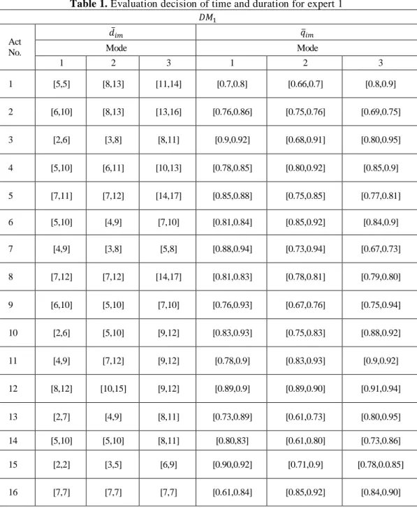
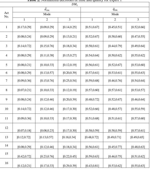
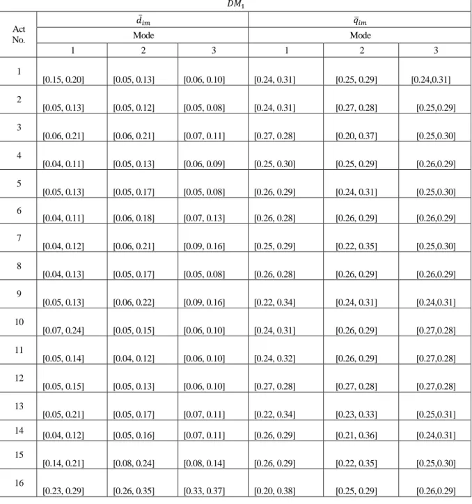
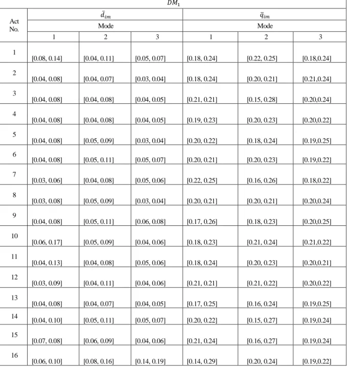
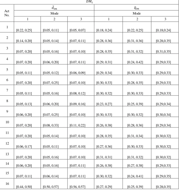
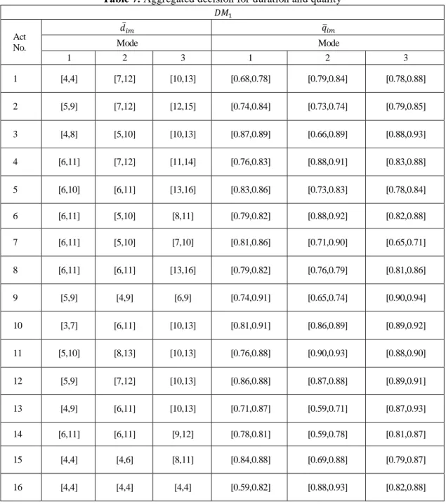
Sprecher, 1996). In this section, the presented GDM method and multi-objective model are solved with an adapted application example from PSPLIB. This application example has 18 activities. In the GDM method, the evaluations of three DMs are reported, and the result of the first DM is shown in table 2. Due to the dummy activities, the result of the 16 activities instead of 18 activities is reported. Then the normalized decision is constructed which is shown in table 1. After that the normalized weighted decision matrix is evaluated, and the result of the normalized weighted decision matrix for DM 1 is shown in table 1. In the next step, the weighted normalized decisions are evaluated which is shown in table 2. The next step is the evaluation of positive ideal decision and two negative ideal decisions which are illustrated in tables 3-5, respectively. The bidirectional projection measure, relative closeness, and the weight of DMs are reported in table 6. Finally, the collective decision is obtained which is shown in table 7.
225
Table 1. Evaluation decision of time and duration for expert 1
𝐷𝑀1 Act
No.
𝑑̅𝑖𝑚 𝑞̅𝑖𝑚
Mode Mode
1 2 3 1 2 3
1 [5,5] [8,13] [11,14] [0.7,0.8] [0.66,0.7] [0.8,0.9]
2 [6,10] [8,13] [13,16] [0.76,0.86] [0.75,0.76] [0.69,0.75]
3 [2,6] [3,8] [8,11] [0.9,0.92] [0.68,0.91] [0.80,0.95]
4 [5,10] [6,11] [10,13] [0.78,0.85] [0.80,0.92] [0.85,0.9]
5 [7,11] [7,12] [14,17] [0.85,0.88] [0.75,0.85] [0.77,0.81]
6 [5,10] [4,9] [7,10] [0.81,0.84] [0.85,0.92] [0.84,0.9]
7 [4,9] [3,8] [5,8] [0.88,0.94] [0.73,0.94] [0.67,0.73]
8 [7,12] [7,12] [14,17] [0.81,0.83] [0.78,0.81] [0.79,0.80]
9 [6,10] [5,10] [7,10] [0.76,0.93] [0.67,0.76] [0.75,0.94]
10 [2,6] [5,10] [9,12] [0.83,0.93] [0.75,0.83] [0.88,0.92]
11 [4,9] [7,12] [9,12] [0.78,0.9] [0.83,0.93] [0.9,0.92]
12 [8,12] [10,15] [9,12] [0.89,0.9] [0.89,0.90] [0.91,0.94]
13 [2,7] [4,9] [8,11] [0.73,0.89] [0.61,0.73] [0.80,0.95]
14 [5,10] [5,10] [8,11] [0.80,83] [0.61,0.80] [0.73,0.86]
15 [2,2] [3,5] [6,9] [0.90,0.92] [0.71,0.9] [0.78,0.0.85]
226
Table 2. Normalized decisions of time and quality for expert 1
𝐷𝑀1 Act
No.
𝑑̅𝑖𝑚 𝑞̅𝑖𝑚
Mode Mode
1 2 3 1 2 3
1 [0.17,0.29] [0.09,0.29] [0.14,0.25] [0.51,0.67] [0.45,0.51] [0.52,0.66]
2 [0.08,0.24] [0.09,0.29] [0.13,0.21] [0.52,0.67] [0.58,0.60] [0.47,0.55]
3 [0.14,0.72] [0.15,0.76] [0.18,0.34] [0.58,0.61] [0.44,0.79] [0.49,0.64]
4 [0.08,0.29] [0.11,0.38] [0.15,0.27] [0.54,0.64] [0.50,0.62] [0.55,0.62]
5 [0.08,0.21] [0.10,0.33] [0.12,0.19] [0.56,0.61] [0.52,0.67] [0.53,0.60]
6 [0.08,0.29] [0.13,0.57] [0.20,0.39] [0.57,0.61] [0.53,0.61] [0.55,0.63]
7 [0.09,0.36] [0.15,0.76] [0.25,0.54] [0.59,0.68] [0.46,0.76] [0.54,0.64]
8 [0.07,0.21] [0.10,0.33] [0.12,0.19] [0.57,0.60] [0.57,0.61] [0.53,0.57]
9 [0.08,0.24] [0.12,0.46] [0.20,0.39] [0.48,0.72] [0.52,0.67] [0.46,0.64]
10 [0.14,0.72] [0.12,0.46] [0.17,0.30] [0.52,0.66] [0.48,0.57] [0.55,0.59]
11 [0.09,0.36] [0.10,0.33] [0.17,0.30] [0.51,0.68] [0.51,0.61] [0.57,0.60]
12
[0.07,0.18] [0.08,0.23] [0.17,0.30] [0.58,0.59] [0.58,0.59] [0.57,0.61]
13 [0.12,0.72] [0.13,0.57] [0.18,0.34] [0.48,0.72] [0.49,0.71] [0.49,0.65]
14 [0.08,0.29] [0.12,0.46] [0.18,0.34] [0.56,0.61] [0.45,0.77] [0.48,0.63]
15
[0.42,0.72] [0.23,0.76] [0.22,0.45] [0.59,0.63] [0.46,0.75] [0.51,0.62]
16
227
Table 3. Ideal decisions of time and quality
𝐷𝑀1 Act
No.
𝑑̅𝑖𝑚 𝑞̅𝑖𝑚
Mode Mode
1 2 3 1 2 3
1
[0.15, 0.20] [0.05, 0.13] [0.06, 0.10] [0.24, 0.31] [0.25, 0.29] [0.24,0.31]
2
[0.05, 0.13] [0.05, 0.12] [0.05, 0.08] [0.24, 0.31] [0.27, 0.28] [0.25,0.29]
3
[0.06, 0.21] [0.06, 0.21] [0.07, 0.11] [0.27, 0.28] [0.20, 0.37] [0.25,0.30]
4
[0.04, 0.11] [0.05, 0.13] [0.06, 0.09] [0.25, 0.30] [0.25, 0.29] [0.26,0.29]
5
[0.05, 0.13] [0.05, 0.17] [0.05, 0.08] [0.26, 0.29] [0.24, 0.31] [0.25,0.30]
6
[0.04, 0.11] [0.06, 0.18] [0.07, 0.13] [0.26, 0.28] [0.26, 0.29] [0.26,0.29]
7
[0.04, 0.12] [0.06, 0.21] [0.09, 0.16] [0.25, 0.29] [0.22, 0.35] [0.25,0.30]
8
[0.04, 0.13] [0.05, 0.17] [0.05, 0.08] [0.26, 0.28] [0.26, 0.29] [0.26,0.29]
9
[0.05, 0.13] [0.06, 0.22] [0.09, 0.16] [0.22, 0.34] [0.24, 0.31] [0.24,0.31]
10
[0.07, 0.24] [0.05, 0.15] [0.06, 0.10] [0.24, 0.31] [0.26, 0.29] [0.27,0.28]
11
[0.05, 0.14] [0.04, 0.12] [0.06, 0.10] [0.24, 0.32] [0.26, 0.29] [0.27,0.28]
12
[0.05, 0.15] [0.05, 0.13] [0.06, 0.10] [0.27, 0.28] [0.27, 0.28] [0.27,0.28]
13
[0.05, 0.21] [0.05, 0.17] [0.07, 0.11] [0.22, 0.34] [0.23, 0.33] [0.25,0.31] 14
[0.04, 0.12] [0.05, 0.16] [0.07, 0.11] [0.26, 0.29] [0.21, 0.36] [0.24,0.31]
15
[0.14, 0.21] [0.08, 0.24] [0.08, 0.14] [0.26, 0.29] [0.22, 0.35] [0.25,0.30]
16
228
Table 4. First negative ideal decisions of time and quality
𝐷𝑀1 Act
No.
𝑑̅𝑖𝑚 𝑞̅𝑖𝑚
Mode Mode
1 2 3 1 2 3
1
[0.08, 0.14] [0.04, 0.11] [0.05, 0.07] [0.18, 0.24] [0.22, 0.25] [0.18,0.24]
2
[0.04, 0.08] [0.04, 0.07] [0.03, 0.04] [0.18, 0.24] [0.20, 0.21] [0.21,0.24]
3
[0.04, 0.08] [0.04, 0.08] [0.04, 0.05] [0.21, 0.21] [0.15, 0.28] [0.20,0.24]
4
[0.04, 0.08] [0.04, 0.08] [0.04, 0.05] [0.19, 0.23] [0.20, 0.23] [0.20,0.22]
5
[0.04, 0.08] [0.05, 0.09] [0.03, 0.04] [0.20, 0.22] [0.18, 0.24] [0.19,0.25]
6
[0.04, 0.08] [0.05, 0.11] [0.05, 0.07] [0.20, 0.21] [0.20, 0.23] [0.19,0.22]
7
[0.03, 0.06] [0.04, 0.08] [0.05, 0.06] [0.22, 0.25] [0.16, 0.26] [0.18,0.22]
8
[0.03, 0.08] [0.05, 0.09] [0.03, 0.04] [0.20, 0.21] [0.20, 0.21] [0.20,0.24]
9
[0.04, 0.08] [0.05, 0.11] [0.06, 0.08] [0.17, 0.26] [0.18, 0.23] [0.20,0.25]
10
[0.06, 0.17] [0.05, 0.09] [0.04, 0.06] [0.18, 0.23] [0.21, 0.24] [0.21,0.22]
11
[0.04, 0.13] [0.04, 0.08] [0.05, 0.06] [0.18, 0.24] [0.20, 0.23] [0.20,0.21]
12
[0.03, 0.09] [0.04, 0.11] [0.04, 0.06] [0.21, 0.21] [0.21, 0.22] [0.20,0.22]
13
[0.04, 0.08] [0.04, 0.07] [0.04, 0.05] [0.17, 0.25] [0.16, 0.24] [0.19,0.25] 14
[0.04, 0.10] [0.05, 0.11] [0.05, 0.07] [0.20, 0.22] [0.15, 0.27] [0.19,0.24]
15
[0.07, 0.08] [0.06, 0.09] [0.04, 0.06] [0.21, 0.24] [0.16, 0.27] [0.19,0.24]
16
229
Table 5. Second negative ideal decisions of time and quality
𝐷𝑀1 Act
No.
𝑑̅𝑖𝑚 𝑞̅𝑖𝑚
Mode Mode
1 2 3 1 2 3
1
[0.22, 0.25] [0.05, 0.11] [0.05, 0.07] [0.18, 0.24] [0.22, 0.25] [0.18,0.24]
2
[0.14, 0.20] [0.05, 0.14] [0.07, 0.11] [0.28, 0.36] [0.31, 0.36] [0.28,0.35]
3
[0.07, 0.20] [0.05, 0.16] [0.07, 0.10] [0.28, 0.35] [0.31, 0.32] [0.31,0.35]
4
[0.07, 0.20] [0.06, 0.20] [0.07, 0.11] [0.29, 0.31] [0.24, 0.42] [0.29,0.33]
5
[0.05, 0.11] [0.05, 0.12] [0.06, 0.09] [0.29, 0.34] [0.30, 0.33] [0.29,0.33]
6
[0.07, 0.20] [0.07, 0.25] [0.07, 0.10] [0.30, 0.33] [0.28, 0.35] [0.29,0.33]
7
[0.05, 0.11] [0.05, 0.16] [0.08, 0.12] [0.30, 0.32] [0.30, 0.33] [0.29,0.33]
8
[0.05, 0.13] [0.06, 0.20] [0.09, 0.16] [0.23, 0.27] [0.25, 0.39] [0.29,0.34]
9
[0.06, 0.20] [0.07, 0.25] [0.07, 0.10] [0.30, 0.33] [0.30, 0.32] [0.30,0.34]
10
[0.07, 0.20] [0.08, 0.33] [0.11, 0.22] [0.26, 0.38] [0.28, 0.36] [0.29,0.34]
11
[0.07, 0.20] [0.05, 0.14] [0.07, 0.10] [0.28, 0.35] [0.31, 0.34] [0.30,0.32]
12
[0.06, 0.17] [0.05, 0.11] [0.07, 0.10] [0.27, 0.36] [0.30, 0.33] [0.30,0.32]
13
[0.07, 0.20] [0.05, 0.16] [0.07, 0.10] [0.31, 0.31] [0.31, 0.32] [0.30,0.32] 14
[0.06, 0.20] [0.05, 0.16] [0.07, 0.11] [0.26, 0.38] [0.27, 0.38] [0.29,0.33]
15
[0.07, 0.11] [0.06, 0.14] [0.07, 0.11] [0.30, 0.32] [0.24, 0.41] [0.29,0.35]
16
230
Table 6. Bi-directional projection, relative closeness, and weight of experts 𝐵𝑃𝑟𝑜𝑗(𝑌̅∗, 𝑌̅𝑘) 𝐵𝑃𝑟𝑜𝑗(𝑌̅𝑙, 𝑌̅𝑘) 𝐵𝑃𝑟𝑜𝑗(𝑌̅𝐶, 𝑌̅𝑘)
𝑁𝑅𝐶
𝑘 𝜆𝑘𝐷𝑀1 0.768 0.479 0.865 0.364 0.32
𝐷𝑀2 0.739 0.312 0.917 0.375 0.33
𝐷𝑀3 0.694 0.557 0.523 0.391 0.35
Table 7. Aggregated decision for duration and quality
𝐷𝑀1 Act
No.
𝑑̅𝑖𝑚 𝑞̅𝑖𝑚
Mode Mode
1 2 3 1 2 3
1 [4,4] [7,12] [10,13] [0.68,0.78] [0.79,0.84] [0.78,0.88]
2 [5,9] [7,12] [12,15] [0.74,0.84] [0.73,0.74] [0.79,0.85]
3 [4,8] [5,10] [10,13] [0.87,0.89] [0.66,0.89] [0.88,0.93]
4 [6,11] [7,12] [11,14] [0.76,0.83] [0.88,0.91] [0.83,0.88]
5 [6,10] [6,11] [13,16] [0.83,0.86] [0.73,0.83] [0.78,0.84]
6 [6,11] [5,10] [8,11] [0.79,0.82] [0.88,0.92] [0.82,0.88]
7 [6,11] [5,10] [7,10] [0.81,0.86] [0.71,0.90] [0.65,0.71]
8 [6,11] [6,11] [13,16] [0.79,0.82] [0.76,0.79] [0.81,0.86]
9 [5,9] [4,9] [6,9] [0.74,0.91] [0.65,0.74] [0.90,0.94]
10 [3,7] [6,11] [10,13] [0.81,0.91] [0.86,0.89] [0.89,0.92]
11 [5,10] [8,13] [10,13] [0.76,0.88] [0.90,0.93] [0.88,0.90]
12 [5,9] [7,12] [10,13] [0.86,0.88] [0.87,0.88] [0.89,0.91]
13 [4,9] [6,11] [10,13] [0.71,0.87] [0.59,0.71] [0.87,0.93]
14 [6,11] [6,11] [9,12] [0.78,0.81] [0.59,0.78] [0.81,0.87]
15 [4,4] [4,6] [8,11] [0.84,0.88] [0.69,0.88] [0.79,0.87]
231
The aggregated decision determines the duration and quality of the project activities in the presented mathematical model. The proposed mathematical model is solved by the extended solving method, and the result of the time quality trade-off is shown in table 8.
Table 8. The result of time quality trade-off
Z1(Time) Z2(Quality)
optimistic pessimistic optimistic pessimistic
81 127 0.88 0.85
82 128 0.89 0.86
83 129 0.91 0.87
84 130 0.92 0.9
86 131 0.93 0.92
87 132 0.94 0.93
88 133 0.96 0.94
89 134 0.97 0.95
6- Sensitivity analysis
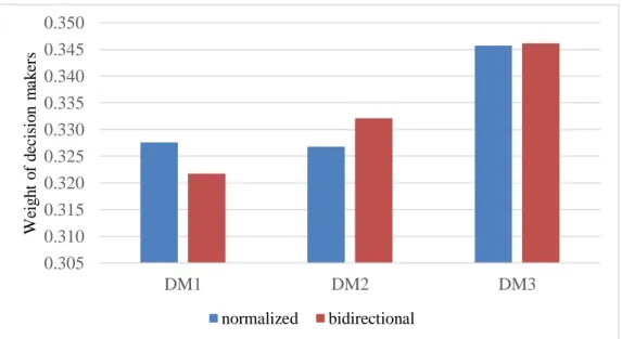
According to figure 1 in both methods DM3 gained the highest weight. The result of using bidirectional and normalized projection shows that the place of DM2 and DM1 are changed. It means by using the bidirectional projection DM2 is gained a higher than DM1 while using the normalized projection DM1 gained a higher weight than DM2. But the difference between these weights can be ignored.
Fig 1. Comparing the result of GDM with the bidirectional and normalized projection
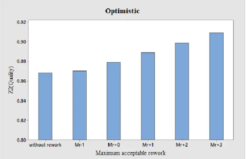
The sensitivity analyses on the maximum acceptable quality level and the time-quality trade-off are provided. First, the increase in maximum acceptable rework (Mr) against the project quality in the optimistic situation is analyzed in figure 2. As the figure 2 shows, when the maximum acceptable rework increases, the project quality becomes higher. This issue happens because of the increase in the maximum
0.305 0.310 0.315 0.320 0.325 0.330 0.335 0.340 0.345 0.350
DM1 DM2 DM3
W
ei
g
h
t
o
f
d
ec
is
io
n
m
a
k
er
s
232
acceptable rework allows activities to have more reworking days. As the reworking leads to a higher quality level for the activities, thus the project quality increases.
Fig 2. Effect of change in acceptable rework on the project quality in optimistic situation
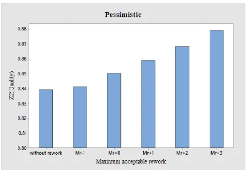
The next analysis is similar to the first one but in the pessimistic situation. Figure 3 shows the effect of the change in the maximum acceptable rework value against the project quality. The result of this figure indicates that the increase in the allowed rework value leads to higher project quality. Although the results of figure 2 and figure 3 illustrate the increasing trend for the project quality but the quality range in the pessimistic and optimistic situations is different. Totally, the result of the optimistic situation shows 3% higher quality level than pessimistic situations.
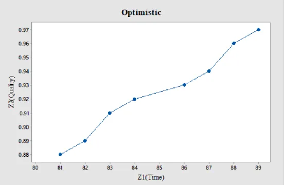
Two remained analyses are about objectives trade-off. First, the effect of time quality trade-off in the optimistic situation is shown in figure 4. Based on figure 4, the higher project quality needs more time. The longer project makespan is due to the more reworking, so this extra reworking in an activity increases the project quality. In all of the real projects, the time-quality trade-off happens, and DMs have significant attention to this issue. As the time and quality of the activities are intervals, the effect of the time quality trade-off in the pessimistic situation should be analyzed too. The result of the time quality trade-off in the pessimistic situation is shown in figure 5.
Figure 5 confirms that higher project quality needs longer makespan. Actually, the increase in the project quality in the longer project completion time is verified in both situations, optimistic and pessimistic. But the range of the project quality and completion time are different in pessimistic and optimistic situations. For example, in the optimistic situation the project quality by completing project in 86 days is 0.93 while in the pessimistic situation the project needs 132 days to reach the same quality level. To sum up, when the project completion time increases, the project quality increases, and the range of this increase in the pessimistic situation and optimistic situations are different.
233
Fig 3. Effect of change in acceptable rework on the project quality in pessimistic situation
234
Fig 5. Time quality trade-off in the pessimistic situation
7- Conclusions
In this paper, a new combination of group decision making and MRCPSP is presented. In the first step, the duration and quality of the activities are determined based on new group decision-making method with the interval information. In the group decision-making method, the weight of DMs is obtained based on the bidirectional projection between individual decisions with a positive ideal solution and two negative ideal solutions. Then, based on the relative closeness to the positive ideal solution and distance from negative solutions, weight of the experts evaluated and a collective decision made. The collective decision determines the quality and duration of the activities. The presented MRCPSP model has two objectives, minimizing the project completion time, and maximizing the project quality. In the mathematical model, the quality of activity can be increased via reworking. The reworking amount has a direct effect on the precedence constraint, so the effect of the reworking is considered in the mathematical model. The presented mathematical model has two objectives, and some parameters are interval, so the extended solving method based on the goal programming is presented. In this paper, an adapted application example is solved, and some analyses are clearly explained. The results show that higher project quality needs longer makespan. Besides, the maximum acceptable reworking value has a direct effect on the project quality.
For future researches, it is suggested to extend the mathematical model in a multi-project environment. Besides, the budget and cost of the resources can be added to the model. Future research can be also continued on projection-based methods with hybrid information. In addition, more efficient methods for solving the mathematical model can be developed in real-world applications.
235
References
Arditi, D., & Pattanakitchamroon, T. (2006). Selecting a delay analysis method in resolving construction claims. International Journal of project management, 24(2), 145-155.
Babu, A. J. G., & Suresh, N. (1996). Project management with time, cost, and quality considerations.
European journal of operational research, 88(2), 320-327.
Baudry, G., Macharis, C., & Vallee, T. (2018). Range-based Multi-Actor Multi-Criteria Analysis: A combined method of Multi-Actor Multi-Criteria Analysis and Monte Carlo simulation to support participatory decision making under uncertainty. European Journal of Operational Research, 264(1), 257-269.
Birjandi, A., & Mousavi, S. M. (2019). Fuzzy resource-constrained project scheduling with multiple routes: A heuristic solution. Automation in Construction, 100, 84-102.
Birjandi, A., Mousavi, S. M., Hajirezaie, M., & Vahdani, B. (2019). Optimizing and Solving Project Scheduling Problem for Flexible Networks with Multiple Routes in Production Environments. Journal of Quality Engineering and Production Optimization, 4(1), 175-196.
Bodily, S. E. (1979). Note—A delegation process for combining individual utility functions. Management Science, 25(10), 1035-1041.
Bruni, M. E., Beraldi, P., Guerriero, F., & Pinto, E. (2011). A heuristic approach for resource constrained project scheduling with uncertain activity durations. Computers & Operations Research, 38(9), 1305-1318.
Chen, T. Y. (2015). The inclusion-based TOPSIS method with interval-valued intuitionistic fuzzy sets for multiple criteria group decision making. Applied Soft Computing, 26, 57-73.
Chen, T. Y. (2016). An interval-valued intuitionistic fuzzy permutation method with likelihood-based preference functions and its application to multiple criteria decision analysis. Applied Soft Computing, 42, 390-409.
Cheng, M. Y., Tran, D. H., & Cao, M. T. (2016). Chaotic initialized multiple objective differential evolution with adaptive mutation strategy (CA-MODE) for construction project time-cost-quality trade-off. Journal of Civil Engineering and Management, 22(2), 210-223.
Chung, C. K., Chen, H. M., Chang, C. T., & Huang, H. L. (2018). On fuzzy multiple objective linear programming problems. Expert Systems with Applications, 114, 552-562.
Das, S., & Kar, S. (2014). Group decision making in medical system: An intuitionistic fuzzy soft set approach. Applied soft computing, 24, 196-211.
Deli, I. (2015). npn-Soft sets theory and their applications. Ann Fuzzy Math Inform, 10(6), 847-862. Dey, B., Bairagi, B., Sarkar, B., & Sanyal, S. K. (2017). Group heterogeneity in multi member decision making model with an application to warehouse location selection in a supply chain. Computers & Industrial Engineering, 105, 101-122.
236
Dorfeshan, Y., & Mousavi, S. M. (2019). A group TOPSIS-COPRAS methodology with Pythagorean fuzzy sets considering weights of experts for project critical path problem. Journal of Intelligent & Fuzzy Systems, 36(2), 1375-1387.
Dorfeshan, Y., Tavakkoli-Moghaddam, R., Mousavi, S. M., & Vahedi-Nouri, B. (2020). A new weighted distance-based approximation methodology for flow shop scheduling group decisions under the interval-valued fuzzy processing time. Applied Soft Computing, 106248.
Haghighi, M. H., Mousavi, S. M., Antuchevičienė, J., & Mohagheghi, V. (2019). A new analytical methodology to handle time-cost trade-off problem with considering quality loss cost under interval-valued fuzzy uncertainty. Technological and Economic Development of Economy, 25(2), 277-299. Hancerliogullari, G., Hancerliogullari, K. O., & Koksalmis, E. (2017). The use of multi-criteria decision making models in evaluating anesthesia method options in circumcision surgery. BMC medical informatics and decision making, 17(1), 14.
Hazır, Ö., Erel, E., & Günalay, Y. (2011). Robust optimization models for the discrete time/cost trade-off problem. International Journal of Production Economics, 130(1), 87-95.
Hegazy, T., Said, M., & Kassab, M. (2011). Incorporating rework into construction schedule analysis.
Automation in construction, 20(8), 1051-1059.
Hwang, B. G., Thomas, S. R., Haas, C. T., & Caldas, C. H. (2009). Measuring the impact of rework on construction cost performance. Journal of construction engineering and management, 135(3), 187-198. Hwang, C. L., & Yoon, K. (1981). Methods for multiple attribute decision making. In Multiple attribute decision making (pp. 58-191). Springer, Berlin, Heidelberg.
Icmeli-Tukel, O., & Rom, W. O. (1997). Ensuring quality in resource constrained project scheduling.
European journal of operational research, 103(3), 483-496.
Kolisch, R., & Sprecher, A. (1997). PSPLIB-a project scheduling problem library: OR software-ORSEP operations research software exchange program. European journal of operational research, 96(1), 205-216.
Kolisch, R., Sprecher, A., & Drexl, A. (1995). Characterization and generation of a general class of resource-constrained project scheduling problems. Management science, 41(10), 1693-1703.
Konak, A., Coit, D. W., & Smith, A. E. (2006). Multi-objective optimization using genetic algorithms: A tutorial. Reliability Engineering & System Safety, 91(9), 992-1007.
Liao, H., Li, Z., Zeng, X. J., & Liu, W. (2017). A comparison of distinct consensus measures for group decision making with intuitionistic fuzzy preference relations. International Journal of Computational Intelligence Systems, 10(1), 456-469.
Liu, P. (2017). Multiple attribute group decision making method based on interval-valued intuitionistic fuzzy power Heronian aggregation operators. Computers & Industrial Engineering, 108, 199-212. Liu, W. (2016). VIKOR method for group decision making problems with ordinal interval numbers'. International Journal of Hybrid Information Technology, 9(2), 67-74.
237
Liu, Y., Dong, Y., Liang, H., Chiclana, F., & Herrera-Viedma, E. (2018). Multiple attribute strategic weight manipulation with minimum cost in a group decision making context with interval attribute weights information. IEEE Transactions on Systems, Man, and Cybernetics: Systems, 49(10), 1981-1992.
Moghiseh, H., Mousavi, S. M., & Patoghi, A. (2019). A new project controlling approach based on earned value management and group decision-making process with triangular intuitionistic fuzzy sets.
Journal of Industrial and Systems Engineering, 12(3), 177-195.
Mohagheghi, V., & Mousavi, S. M. (2019). A new framework for high-technology project evaluation and project portfolio selection based on Pythagorean fuzzy WASPAS, MOORA and mathematical modeling.
Iranian Journal of Fuzzy Systems, 16(6), 89-106.
Mohagheghi, V., Mousavi, S. M., Antuchevičienė, J., & Dorfeshan, Y. (2019). Sustainable infrastructure project selection by a new group decision-making framework introducing MORAS method in an interval type 2 fuzzy environment. International Journal of Strategic Property Management, 23(6), 390-404. Muritiba, A. E. F., Rodrigues, C. D., & da Costa, F. A. (2018). A Path-Relinking algorithm for the multi-mode resource-constrained project scheduling problem. Computers & Operations Research, 92, 145-154. Nguyen, H. (2016). A new interval-valued knowledge measure for interval-valued intuitionistic fuzzy sets and application in decision making. Expert Systems with Applications, 56, 143-155.
Peng, X., & Liu, C. (2017). Algorithms for neutrosophic soft decision making based on EDAS, new similarity measure and level soft set. Journal of Intelligent & Fuzzy Systems, 32(1), 955-968.
Sonmez, R., & Bettemir, Ö. H. (2012). A hybrid genetic algorithm for the discrete time–cost trade-off problem. Expert Systems with Applications, 39(13), 11428-11434.
Tareghian, H. R., & Taheri, S. H. (2006). On the discrete time, cost and quality trade-off problem.
Applied mathematics and computation, 181(2), 1305-1312.
Tian, Z. P., Zhang, H. Y., Wang, J., Wang, J. Q., & Chen, X. H. (2016). Multi-criteria decision-making method based on a cross-entropy with interval neutrosophic sets. International Journal of Systems Science, 47(15), 3598-3608.
Tsao, C. Y., & Chen, T. Y. (2016). A projection-based compromising method for multiple criteria decision analysis with interval-valued intuitionistic fuzzy information. Applied Soft Computing, 45, 207-223.
Turner, J. R., & Keegan, A. (1999). The versatile project-based organization: governance and operational control. European management journal, 17(3), 296-309.
Wang, G. A., Jiao, J., Abrahams, A. S., Fan, W., & Zhang, Z. (2013). ExpertRank: A topic-aware expert finding algorithm for online knowledge communities. Decision support systems, 54(3), 1442-1451. Wang, L., & Fang, C. (2012). An effective estimation of distribution algorithm for the multi-mode resource-constrained project scheduling problem. Computers & Operations Research, 39(2), 449-460.
238
Wang, Z. J., & Li, K. W. (2012). An interval-valued intuitionistic fuzzy multiattribute group decision making framework with incomplete preference over alternatives. Expert Systems with Applications, 39(18), 13509-13516.
Weglarz, J., Józefowska, J., Mika, M., & Waligóra, G. (2011). Project scheduling with finite or infinite number of activity processing modes – A survey. European Journal of Operational Research, 208, 177–205.
Wei, G., Lin, R., Zhao, X., & Wang, H. (2014). An approach to multiple attribute decision making based on the induced Choquet integral with fuzzy number intuitionistic fuzzy information. Journal of Business Economics and Management, 15(2), 277-298.
Wuliang, P., & Chengen, W. (2009). A multi-mode resource-constrained discrete time–cost trade-off problem and its genetic algorithm based solution. International journal of project management, 27(6), 600-609.
Xu, J., Zheng, H., Zeng, Z., Wu, S., & Shen, M. (2012). Discrete time–cost–environment trade-off problem for large-scale construction systems with multiple modes under fuzzy uncertainty and its
application to Jinping-II Hydroelectric Project. International Journal of Project Management, 30(8), 950-966.
Xu, Z., & Da, Q. (2004). Projection method for uncertain multi-attribute decision making with preference information on alternatives. International Journal of Information Technology & Decision Making, 3(03), 429-434.
Xu, Z., & Hu, H. (2010). Projection models for intuitionistic fuzzy multiple attribute decision making. International Journal of Information Technology & Decision Making, 9(02), 267-280.
Yang, Q., & Du, P. A. (2015). A straightforward approach for determining the weights of decision makers based on angle cosine and projection method. International Journal of Social, Behavioral, Educational, Economic, Business and Industrial Engineering, 9(10), 3127-3133.
Yang, Q., Du, P. A., Wang, Y., & Liang, B. (2018). Developing a rough set based approach for group decision making based on determining weights of decision makers with interval numbers. Operational Research, 18(3), 757-779.
Yu, G. F., Li, D. F., & Fei, W. (2018). A novel method for heterogeneous multi-attribute group decision making with preference deviation. Computers & Industrial Engineering, 124, 58-64.
Yue Z (2014) TOPSIS-based group decision-making methodology in intuitionistic fuzzy setting. Inf Sci 277:141–153.
Yue, C. (2016). A geometric approach for ranking interval-valued intuitionistic fuzzy numbers with an application to group decision-making. Computers & Industrial Engineering, 102, 233-245.
Yue, C. (2018). A novel approach to interval comparison and application to software quality evaluation.
Journal of Experimental & Theoretical Artificial Intelligence, 30(5), 583-602.
Yue, C. (2018). Normalized projection approach to group decision-making with hybrid decision information. International Journal of Machine Learning and Cybernetics, 9(8), 1365-1375.
239
Yue, C. (2019). An interval-valued intuitionistic fuzzy projection-based approach and application to evaluating knowledge transfer effectiveness. Neural Computing and Applications, 31(11), 7685-7706.
Yue, Z. (2011). Deriving decision maker’s weights based on distance measure for interval-valued intuitionistic fuzzy group decision making. Expert Systems with Applications, 38(9), 11665-11670. Yue, Z. (2012). Developing a straightforward approach for group decision making based on determining weights of decision makers. Applied Mathematical Modelling, 36(9), 4106-4117.
Yue, Z. (2013). An intuitionistic fuzzy projection-based approach for partner selection. Applied Mathematical Modelling, 37(23), 9538-9551.
Yue, Z. (2014). TOPSIS-based group decision-making methodology in intuitionistic fuzzy setting.
Information Sciences, 277, 141-153.
Yue, Z., & Jia, Y. (2015). A group decision making model with hybrid intuitionistic fuzzy information.
Computers & Industrial Engineering, 87, 202-212.
Yue, Z., & Jia, Y. (2017). A direct projection-based group decision-making methodology with crisp values and interval data. Soft Computing, 21(9), 2395-2405.
Zavadskas, E. K., Bausys, R., Kaklauskas, A., Ubarte, I., Kuzminske, A., & Gudiene, N. (2017). Sustainable market valuation of buildings by the single-valued neutrosophic MAMVA method. Applied Soft Computing, 57, 74-87.
Zhang, X., Jin, F., & Liu, P. (2013). A grey relational projection method for multi-attribute decision making based on intuitionistic trapezoidal fuzzy number. Applied Mathematical Modelling, 37(5), 3467-3477.