Development of PSPO Simulation Optimization Algorithm

Vol. 5, No. 3, pp128-141 Fall 2011

Development of PSPO Simulation Optimization Algorithm

Zohreh Omranpour1*, Farhad Ghassemi-Tari2

Industrial Engineering Department, Sharif University of Technology, Tehran 14588-89694, Iran 1_{[email protected],} 2_{[email protected]}

ABSTRACT

 

In this article a new algorithm is developed for optimizing computationally expensive simulation models. The optimization algorithm is developed for continues unconstrained single output simulation models. The algorithm is developed using two simulation optimization routines. We employed the nested partitioning (NP) routine for concentrating the search efforts in the regions which are most likely contained the global optimum, and we used the experimental design concept for selecting most promising points. Then we integrated the Particle Swarm Optimization (PSO) routine as the searching mechanism of the developed algorithm to single out the best point (optimal or a near optimal solution). Through these integrations, an algorithm was developed which is capable of optimizing digital simulation models. The efficiency of the developed algorithm was then evaluated through a computational experiment. Ten test problems were selected from the literature and the efficiency of the PSPO algorithm was compared by two well-known algorithms. The result of this experiment revealed that the developed algorithm provided a more accurate result comparing to these algorithms.

Keywords: Simulation optimization, Nested Partition Algorithm, Sequential Experimental

Design, Particle Swarm Optimization Algorithm.

1.INTRODUCTION

Systems designers and decision makers usually employ a designing tool which has the highest performance at lowest cost. Modeling and simulation of system design tradeoff is good preparation for design and engineering decisions in real world jobs. Using Digital computer simulation models for designing a system or performing sensitivity analysis, has been very successful. However procedures for obtaining the best performance measures of computer simulation models has not yet been reached to a unified robust approach.

In the digital computer simulation models, analytical expression for input/output relationship is generally unavailable and therefore conducting the performance evaluation is very difficult. Based on Barton and Meckesheimer(2006), simulation optimization is defined as a repeated analysis of simulation models with different values of design parameters, in an attempt to identify best simulated system performance. Since 1950, when simulation optimization has introduced as a new

       

*_{Corresponding Author}

research area, many practical problems formulized as simulation optimization problems and a quite number of research efforts were conducted to solve these problems. Some recent efforts are the works of Santos and Santos (2009), Liu and Maghsoodloo (2011), Liu (2010) and Kleijnen (2010). Also a number of softwarepackages have been developed with the ability of simulation optimization and have been added to some well-known simulation software. However it seems there is still needs to conduct more research for developing new robust high performance methods. Recent surveys in this field are accomplished by Fu and Glover (2005), Tekin andSabuncuoglu (2004), Henderson and Nelson (2006) and Kleijnen (2008).

Since simulation models have stochastic responses, simulation optimization approaches are considered as difficult tasks. Due to its stochastic nature, the output must be estimated by making some replications and then calculating the average value of the outputs over these replications. These types of problems combine the existing difficulties of deterministic optimization, with the stochastic nature of simulation outputs (Hurrion, 1997). In practice, the objective function relations are not expressed explicitly. Therefore the simulation models are considered the black-box models, in which determining the best combination of input variables that provides the best performance measure is often computationally expensive.

Using metamodel search method for optimizing simulation models has been focused on some well-known algorithms like the genetic, simulated annealing, neural network, and particle swarm optimization algorithms. Although nested portioning (NP) has been used in different areas with successful results, the number of similar works which conducted for NP algorithm is very low. Based on Shi and Ólafsson (2008) the NP results significantly depend on the method of sampling and low quality samples can affect the final result.

In this article we focus on the simplest optimization problem which is an unconstrained simulation model with continuous variables and a single output. We aim to minimize the expected value of this univariate output. Despite the simplicity, these kinds of problems have many applications in practice. Examples are (s,Q)inventory management simulation, inventory production simulation models in logistics and operation management and queuing simulation models (Kleijnen, 2008). The mathematical presentation of the problem is as follow:

)) ( ( minE Y x

x (1)

d j

u x

lj ≤ j ≤ j for 1,2,..., (2)

Wherex=[x1, x2,…,xd]T denotes a d-dimensional input vector andYindicates the output value. The

expected value in the objective function is estimated by simulation and we consider only box constraints whereljanduj are the lower and upper bounds of the input variablesxj respectively. Since

the output of the simulation models is stochastic, we consider this problem and we artificially add some noises to its objective function in order to consider a more realistic problem.

Having this type of problem, we developed an algorithm for optimizing the stochastic version of this problem. Since the main structure of the developed algorithm is the particle swarm optimization algorithm,and since we partition the feasible space iteratively for conduction the search mechanism, we named our algorithm as Particle Swarm Partitioning Optimization algorithm or PSPO algorithm. The rest of this article is organized as follow. In section 2 we review the pure nested partition

method briefly. In section 3 the particle swarm optimization method which will be used in sampling part of NP algorithm is described. In section 4, we present a thorough discussion of the developed algorithm. Finally, section 6 presents a computational experiment, in which the efficiency of the developed algorithm is evaluated.

2.NESTEDPARTITION METHOD

One of the powerful population based metaheuristics which can be used for solving large-scale optimization problems is nested partition method. This method is first introduced by Shi and Ólafsson (1998) inspired by adaptive partitioned random search (Tang, 1994) and branch and bound algorithm. Portioning the solution space and concentrating the search in some regions, which are most likely contain the global optimum, has been the key idea in developing NP algorithm.

In each iteration, the space solution is split into two regions, a “most promising region” and a “complementary region”. By the use of a predetermined partitioning method, the most promising region by itself is partitioned into some sub-regions.

We use the following notations for representing the solution space. Let:

 The whole feasible region

K Number of iterations

(k) Most promising region in the kth _iteration

 /(k) Complementary or surrounding region of the most promising region

M The number of sub-region obtained by reapportioning the most promising region

I Promising index; which is an index showing the best objective value of each region. In each iteration of the algorithm, the feasible space is partitioned into(k)and /(k). Then,(k) is reapportioned into the M sub-regions. These new sub-regions with complementary region form

M+1 regions. In order to find the next most promising region which has the best output value, some samples are taken randomly from each region and their function values are calculated. The best function value in each region is designated as the best index of that region. If one of the sub-regions has the best I, this sub-region is selected as the next promising region. Otherwise if the best I

belongs to the complimentary region, it shows that this iteration has had incorrect move, and algorithm backtrack to the union of(k)and /(k).

It should be noted that, in the initial iteration, we usually do not have any information regarding the output vale and therefore we partition the feasible region into M regions with equally likely of being promising region. Since in this iteration there is no complimentary region, algorithm just partitions feasible region in to M sub-regions and it performs the above procedure in these M+1 regions. Shi and Ólafsson (1998) proved that for any combinatorial optimization problem (COP) their method converges with probability of one to a global optimum in a finite computational time. One of the advantages of this algorithm which provides high-quality solutions is applying both global search by sampling from the entire feasible region and local search by calculating the promising index for all regions. Their method also can be run in parallel processors and so has the ability to use parallel processing systems.

NP method has been used in both deterministic (Shi and Ólafsson, 1998) and stochastic (Shi and Ólafsson, 2000) optimization problems. It also has been successfully applied in many areas, such as planning and scheduling, logistics and transportation, supply chain design, data mining and health

care and task assignment. This method also is used for solving some difficult optimization problems like traveling sales man problem (Shiet al., 1999) and production scheduling problems (Ólafsson and Shi, 1998). More details discussion regarding its applications can be found in Shi and Ólafsson (2008) and Chen (2009).

Prior works considering NP hybrid show that incorporating other heuristics in sampling stage of the NP is considerably more efficient than a simple random generation of feasible solutions.

Using linear programming or some metaheuristic algorithms like Genetic algorithm or Ant colony for improving the quality of initial samples is common in the NP literature. The latest article in this area is Al-Shihabi and Ólafsson (2010). Other efforts are Pi et al.(2008) which used the linear relaxation (LR) solution for generating high quality samples, Shi and Ólafsson (2008),Shi et al.(1999), and Al-Shihabi (2004).

3. PARTICLESWARMOPTIMIZATION

The PSO method is a global population-based metaheuristicwhich developed by Kennedyand Eberhart (1995), Kennedy and Eberhart (1995) and Eberhart and Kennedy (1995) for optimizing nonlinear programming problems. The key idea of this algorithm was derived from movement of flying birds.

In each iteration, there is a population (swarm) which consists of some particles. These particles are representative of solution points in the feasible region. Each particle position and velocity of its movement is updated based on the performance of the last recognized particle with the best performance and the best performance obtained by any other particles.

The most important advantage of this method comparing with other population based algorithms is its flexibility for balancing local and global search. Other advantages like robustness, its simplicity, quicker convergence, and computationally lower required memory are justifications of using this method in a wide range of optimization problems.

In first iteration of PSO algorithm, a population of solutions is randomly produced. Then a random velocity is allocated to each elements of this population. In ith _{iteration, the best result of particle j is}

represented by Pbestiand the best global result shows by Gbesti. By repeating the iterations n times,

we will have:

}

,

,

,

{

_{i1 i2 in}

i

optimum

Pbest

Pbest

Pbest

Pbest





}

,

,

,

{

Gbest

₁

Gbest

₂

Gbest

_n

optimum

Gbest





The particle’s velocity plays the most important role in searching process. A velocity is assigned to particle r based three factors as below:

 Current position (which depends on previous velocity).

 Movement toward the best position of particle r.

 Movement toward the best position of all other particles in the population. The position ( t

r

X ) and velocity ( t r

)

(

)

(

1 1

2 2 1 1 1 1

1    



_

_

_

_

_

_

_

_





t r t r t r t r t r t

r

w

V

c

rand

Pbest

X

c

rand

Gbest

X

V

(3)

1 1  

_



t r t r t

r

X

V

X

(4)

Where wis called inertia weight which balances local and global search, i.e. it controls exploration and exploitation, and it has an important effect on algorithm convergence (Shi and Eberhart, 1998). The value ofwis calculated as below:

t

t

w

w

w

w

t    







max min max max

)

(

(5) Where t is the iteration number andtmaxis the maximum number of iterations. Shi and Eberhart

(1998) assigned the values of 0.9 and 0.4 towmaxandwminrespectively. c1 and c2 are acceleration

coefficients which called cognitive (the private thinking of particles) and social (collaboration between particles) parameters respectively. They are positive constant and are not independent of each other while the summation of these two should be less than a constant value. Shi and Eberhart (1998) state that c1 and c2 can be fine-tuned if we assign them an equal valueof 2 (c1=c2= 2). Finally

rand1and rand2 are two random numbers with a uniform distribution.

4. DEVELOPMENTOF PSPO ALGORITHM

Thedeveloped algorithm is a hybrid metheuristic algorithm of nested partition method, which benefits of quick convergence for large scale problems with high computational efforts. We also used the advantages of the PSO algorithm for its simplicity and its good local search ability.

Assuming simulation runs are computationally time consuming, we use a sequential experiment design for selecting most promising pints and also we select the number of simulation replications based on a relative precision requirement.

Figure 1 demonstrates a flow diagram for the developed algorithm. According to Figure 1, PSPO algorithm is an iterative process which starts by an initial experiment design (step1). Then it partitions the feasible space (step 2) and samples from each partition considering previous design and using max-min Latin Hyper Cube Sampling (LHS) design (step3). The sample points are then improved by PSO algorithm (step4). Using the method of Liu (2010), the algorithm determines the number of simulation iterations and then executes simulation model for the sample points (step5). Computing the fitness value for each partition and determining the best partition (the most promising partition) and consequently the best point are conducted in the next step of the algorithm (step 6). Actually this point is used for re-partitioning space and adds this space to the experiment design, which is used for the next sampling process (step7). In step 8 we check whether there is any significant improvement in the objective function value. If there is any improvement the algorithm loop back to step 3, otherwise it check whether the value ofImax

, which is the maximum number of replications for the unimproved objective function value, is reached. If theImax_{criterion is satisfied,}

computation process is stopped, otherwise it loop back to step3.

In the remaining of this section, each step of the developed algorithm will be described in more detail.

Figure 1 The flow diagram of PSPO

Step1: Performing the initial experiment design

The first step of the PSPO algorithm is designed for generating the initial simulation observations, based on a statistical sampling. Selecting an efficient experiment design is an important step in the process of optimizing expensive simulation models and can affect the PSPO algorithm performances.

Based on the assumption that there is no former information about output values, we employed a space-filling experimental design, which called max-min LHS (Kleijnen, 2008), while checking the box constraints. This initial experimental design will then be updated sequentially, since there would be the possibility of adding some more design points based on the complexity of the response surface.

Step2: Initial partitioning

In this step, experimental area is partitioned. Most of the articles that have been developed based on NP method are applied for discrete problems. We used the idea proposed by Kabirian (2006) and modified the NP method for using in the continuous cases. For initial partitioning we divided the range of each variable, which is defined by the box constraint, into two halves. Through this way each variable’s dimension is divided into two equal parts. More detail description of this partitioning method is presented in step7.

Step3: Sampling from partitions

After defining partitions boundaries,

N

uniform random sampling procedure is used for each partition. For this sampling we consider previous experiment design and add more design points (if needed) to them using max-min LHS. The max-min LHS design helps us to place new points such that the minimal distance to any other points is maximized. By this method we construct a set of best design points which will be used in next iterations.

Our main motivation for using max-min LHS for generating samples is twofold. First, the max-min design is certainly space-filling, but not necessarily non-collapsing (Husslag, 2006). Second, it has been widely used in the area of computer simulation because by the use of the sequential experimental design the number of simulation evaluation is reduced.

Step4: Improving samples using PSO

The PSO algorithm is used to improve the quality of initial samples and generate feasible solutions which improve the effectiveness and efficiency of NP algorithm. Suppose we show N initial random samples in the jth _{partition by}



jN



I j I j I j

I

x

x

x

D

_

1

,

2

,...,

_{. Using PSO method, we generate a sequence}

of improving solutions until no further improvement is possible. The final solutions which are more likely to be near optimal region is shown by

D

_Fj

_



x

_Fj1

,

x

_Fj2

,...,

x

_FjN



_{. By using high quality samples}

we increase the probability of selecting correct partition and making correct moves. It should be considered that in next iterations we will have five partitions for sampling. More details provide in step7.

Step5: Simulating the design points

In this step the population obtained in the previous step is simulated. Due to the stochastic nature of simulation models, the output values have some noises. We therefore should obtain an average of simulation outputs over the number of replications. If we denoteni as the number of simulation runs

in a design pointxi, the average will be obtained by:

 

 

i n

k i k i

k

n x w x

W

i





 1 ₍₆₎

simulation run (replication) in order to reduce the output variance, we used the method which was developed by Liu (2010). In this method at first we performed

n

₀ replications for every design pointxi. Then we calculated meanݓഥሺݔ௜ሻand the varianceS2(xi) of these replications. We targeted a

relative precision for simulation outputγ and then determined the total replication sizeniin each

design point. The relative precision forni replication in design pointxi was calculated

by

l

(

xi,ni;α)/|w(xi)| which we required it to be less thanγ. Where

l

(

xi,ni;α) is a half-width of the(1-α)

confidence interval for outputw(xi). We then let: (Kelton, 2007)











  1 ) ( ; , i i i x W n x l ₍₇₎

And finally we calculatednias follow:





 

 

_                            2 0 2 1 , 1 0 1 , max i i n i x W x S t n n





_ (8)

As the result,ni-n0more replication runs in the design pointxishould be executed. After determining

design points and number of replications in each design point, simulation of all the design points can be executed.

Step6: Determining winner partition and near optimal solution

For estimating promising index and finally determining the winner partition (the next most promising region), let us first use the results of simulation runs which is obtained from previous step and showed it by

Y

 

x

_Fj for ith sample in jth partition. The best answer for each partition is designated as the fitness coefficient for that partition. The fitness coefficient for minimization problems it is computed as follow:

 

 

 N

i ji F

j Y x

Y ,.., 2 , 1 min  



forj_=1,2,3,4,5. (9)

The partition with the best overall fitness coefficient is chosen as the next most promising partition:

 

j

k Y

j arg



ˆ _{ forj=1,2,3,4,5. (10)}

If this index corresponds to a sub region of(k),



ˆj_k4



we let this to be the next most promising

partition:



k



 

k

k j

ˆ

1





  (11)

But if it belongs to complementary region we backtrack to previous iteration:



k



1

 





k



1



We save all partitions features including a backtrack-flag for each iteration. If in one of the iterative process, it is backtracked to previous partition, we set this flag on. This flag is used for calculating the number of iterations that algorithm is backtracked, and is used for terminating the iterative process.

We also record the best point which is obtained in each iteration. The index of the best point in jth

partition is obtained as follow:

 

ji F N i

i

x

j

,..., 2 , 1

min

arg

ˆ





forj_=1,2,3,4,5. (13)

We designate the best overall point as jkijk F opt

k x

x  ˆˆ which will be used in next partitioning (step 7). We also compare this point with the best answer which is obtained so far (xopt_{) and we record the}

point which has the best performance measure.

Step7: re-partitioning solution space

In this step the best answer point which is obtained from previous step (xopt_{) will be added to the}

experimental design. This new experimental design is used promising samples in next iterations.If the current best point belongs to the complementary region we back track and we use previous partitioning; but if this point belongs to the promising region, we use this point for partitioning the promising region into four new partitions (four rectangles) somehow that the point becomes one of the corner of these rectangular while the other corners are kept as the corners of the promising region. It is clear that these regions may not have equal area. All the remaining parts of the region except these four partitions are aggregated together and will be formed as the complementary partition. Having these five partitions, we proceed to step 8.

Step 8: Checking stopping rule

The PSPO algorithm is iteratively proceeds until no significant improvement is reached. In order to check this condition, we compare objective function value of current best point

 

opt

k

x

W with the

best point obtained so far



_W

 

_xopt



_{. For this aim we compute the t -student prediction error as}

follow:

   





 



opt





 

opt



k

opt opt

k

x W x

W

x W x

W t





ˆ ˆ

0

 

 (14)

Current best point is accepted as the best near optimum point, only ift0≤t1-α,df wheredfis degree of

freedomand calculated as follow:



n

k

n

opt



df



min

,

In our experiments we setα=0.1 and also set a threshold for maximum number of iterations for the un-improvement replications (Imax_{), by which we terminate the iterative process. The values of these}

parameters set by user considering the problem type. In our experiment we assigned the value of 30 to this threshold (Imax_{=30). If this threshold is reached, the iterative process is terminated and the}

goes to Step3.

5.COMPUTATIONAL EXPERIMENT

In simulation optimization literature a list of test problems has been introduced which can be used for evaluating the efficiency of the developed algorithm. Unfortunately, none of these test problems have the stochastic nature. In the other hand we know that the simulation output has stochastic nature and these test problems can not directly be used for the evaluation purposes. In order to employ these test problems for the simulation environment, we used these test problems and we added some artificial noise to their objective function relations. However the important advantages of using these test problems are: they represent an unbiased list of problems as a benchmark and their functional relations have enough complexity to represent a simulation model output.

The computational experiment was conducted using 10 unconstraint test problems which were presented in the literature. These test problems are as follows:

1. P1; which has just one global minimum, with the following mathematical form:



1



1 _{2 2}

1 2 1 x P x x 

  ,  2 xj 2, for j 1, 2

2. P2; which has one local minimum and one global minimum with the following mathematical form:

















 









2

2 2 ₁ 3 5 2 2

2 1 1 2 1 2 1 2

2 2

1 2

1

3 1 exp 1 10 ₅ exp ₃

exp 1 -3 _j 3 for 1, 2

x

P x x x x x x x

x x x j

  

      __ _  _   

      

3. P3; which has two local minimum and one global minimum, with the following mathematical form:





















 









2

2 2 ₁ 3 5 2 2

3 1 1 2 1 2 1 2

2 2

1 2

1

10 1 exp 1 15 ₅ exp ₃

exp 1 -3 _j 3 for 1,2 x

P x x x x x x x

x x x j

  

       _{ }  _   

 

 

      

4. P4; which is called Six Hump Camelbalck (SHC) has six local minimum and two global minimum, with the following mathematical form:





4

2 ₁ 2 2 2

4 4 2.1 1 x ₃ 1 1 2 4 4 2 2 3 j 3 for 1, 2

P _  x  _x x x    x x  x  j 

 

5. P5; which called Himmelblau function (Hmb) and has several local minimum and one global minimum with the following mathematical form:



11

 

7



0.1





3

 

2



2



-6 6 for 1,2

2 2 1 2 2 2 1 2 2 2 1

5 x x   x x   x   x   x  j

6. P6; which has several local minimum and one global minimum, with the following mathematical form:





2 2

6 1 2 2 0.3cos 3 2 0.7 100 j 100 for 1, 2

P x  x  x   x  j 

7. P7; which called Booth function and has several local minimum and one global minimum with the following mathematical form:



 

2



2

7 1 2 2 7 2 1 2 5 100 j 100 for 1, 2

P  x  x   x x   x  j 

8. P8; which called Michalewics function and has several local minimum and one global minimum with the following mathematical form:

 

20 ₁2

 

20

 

22

8 1 2

2

sin sin x sin sin x -100 _j 100 for 1, 2

P   x _{  } x _{ } _ x  j 

  _{ }

9. P9; which called Sphere function and has no local minimum except the global one with the following mathematical form:

2 2 2 1 9

x

x

P





, 5.12xj 5.12, for j 1, 2

10. P10; which called Brownian function and has three global minimum with the following mathematical form:

 

 



 



 

2 2

10 2 5 ₄ 2 1 5 1 6 10 1 1₈ cos 1 10 -5.12 j 5.12 for 1, 2

P x x _ x _ x x j



   

 

 _ _        

 _{ } 

 

Each test problem was solved using the developed algorithm and two well-known algorithms, NP algorithm and PSO algorithm, selected from literature. To overcome the problem of stochastic output of the simulation models, twenty replication of simulation model was considered and the test problems are solved by each method.

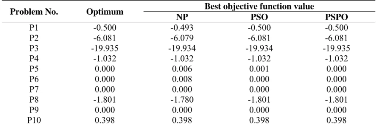
Tables 1 and 2 summarize the results of the computational experiments. Table1 represents the optimal values of the test problems and the best objective function value of twenty replications, which was obtained by using three algorithms. As it is seen, the developed algorithm provides the best results comparing to the other two well-known algorithms. It is interesting to note that, the developed algorithm provides the optimal value of the objective function for all the test problems. Table 2 represents the optimal values of the test problems and the average objective function value over twenty replications, which was obtained by using three algorithms. As it is seen, the developed algorithm also provides the best results comparing to the other two well-known algorithms. It is also interesting to note that, the developed algorithm on average provides the optimal value of the objective function for six of the test problems, and for the rest it provides the average objective function value very close to the optimal value (the deviation from optimal value is less than .0007 or 0.07 percent).

Table 1 Best objective function value obtained comparing to other methods

Problem No. Optimum Best objective function value

NP PSO PSPO

P1 -0.500 -0.493 -0.500 -0.500 P2 -6.081 -6.079 -6.081 -6.081 P3 -19.935 -19.934 -19.934 -19.935 P4 -1.032 -1.032 -1.032 -1.032 P5 0.000 0.006 0.001 0.000 P6 0.000 0.008 0.000 0.000 P7 0.000 0.000 0.000 0.000 P8 -1.801 -1.780 -1.801 -1.801 P9 0.000 0.000 0.000 0.000 P10 0.398 0.398 0.398 0.398

Table 2 Average objective function value obtained comparing to other methods Problem No. Optimum Average objective function over replications

NP PSO PSPO

P1 -0.500 -0.344 0.498 -0.500 P2 -6.081 -6.080 -5.670 -6.080 P3 -19.935 -19.916 -19.935 -19.935 P4 -1.032 -1.031 -1.031 -1.031 P5 0.000 1.350 1.506 0.002 P6 0.000 0.000 0.488 0.000 P7 0.000 0.080 0.000 0.000 P8 -1.801 -1.733 -1.681 -1.800 P9 0.000 0.000 0.000 0.000

P10 0.398 0.498 0.399 0.398

10. CONCLUSION

In this paper, a heuristic algorithm was developed for conducting the optimization process of the stochastic simulation models. We integrated two algorithmic concepts of the nested portioning routine and particle swarm optimization routines for developing this algorithm. We called our developed algorithm particle swarm portioning optimization (PSPO) algorithm.

The efficiency of the PSPO algorithm was then evaluated through computational experiment. Two well-known algorithms, NP algorithm and PSO algorithm was used for comparing their objective function values by the PSOP algorithm. 10 test problems are selected from the literature and solved via the PSOP algorithm and these two algorithms. The results obtained from this experiment were revealed that the PSOP algorithm can provide much better objective function values comparing to these two algorithms. It also revealed that PSPO can mostly provide the optimal objective value or provide the results which are very close to the optimal objective value (the maximum deviations of the test problems’ results from optimal was less than 0.0007).

References

[1] Al-shihabi S. (2004), Ants for sampling in nested partition algorithm; Proceeding of 16th _European Conference on Artificial Intelligence, Valencia, Spain; 11-18.

[2] Al-shihabi S., Ólafsson S. (2004), A hybrid of Nested Partition, Binary Ant System, and linear programming for the multidimensional knapsack problem; Computer & Operation Research 37(2); 247-255.

[3] Barton R.R., Meckesheimer M. (2006), Metamodel-based simulation optimization; Handbooks in Operations Research and Management Science13, Elsevier/North Holland.

[4] Chen W., Pi L., Shi L. (2009), Optimization and logistics challenges in the enterprise; Springer Optimization and its Application 30(2); 229-251.

[5] Eberhart R.C., Kennedy J. (1995), A new optimizer using particle swarm theory; Proceeding of 6th International Symposium on Micro Machine and Human Science, Nagoya, Japan; 39-43.

[6] Fu M.C., Glover F.W., April J. (2005), Simulation optimization: a review, new developments, and applications; Proceedings of the 2005 Winter Simulation Conference, New Jersey, USA; 83-95. [7] Henderson S.G., Nelson B.L. (2006), Handbooks in Operations Research and Management Science13,

Elsevier/North Holland.

[8] Hurrion RD. (1997), An example of simulation optimization using a neural network metamodel: finding the optimum number of kanbans in a manufacturing system; Journal of the Operational Research Society 48(11); 1105-1112.

[10] Kabirian A. (2006), A review of current methodologies and developing a new heuristic method of simulation optimization; M.Sc. Dissertation, Sharif University of Technology, Tehran, Iran.

[11] Kelton W.D., Sadowski R.P., Sturrock D.T. (2007), Simulation with Arena, 4th Ed.; McGraw-Hill. [12] Kennedy J., Eberhart, R.C. (1995), Particle swarm optimization; Proceeding of the IEEE International

Conference on Neural Network4; 1942-1948.

[13] Kleijnen J.P.C., van Beers W., van Nieuwenhuyse I. (2010), Constrained optimization in expensive simulation: Novel approach; European Journal Of Operation Research 202(1); 164-174.

[14] Kleijnen J.P.C. (2008), Design and Analysis of Simulation Experiments; New York: Springer Science, Business Media.

[15] Kleijnen J.P.C. (2008), Response surface methodology for constrained simulation optimization: An overview; Simulation Modeling Practice and Theory 16(1); 50-64.

[16] Liu H., Maghsoodloo S. (2011), Simulation optimization based on Taylor Kriging and evolutionary algorithm; Applied soft Computing 11(4); 3451-3462.

[17] Liu M., Nelson B.L., Staum J. (2010), Simulation on demand for pricing many securities; Proceedings of the 2010 Winter Simulation Conference; 2782-2789.

[18] Shi Y., Eberhart RC. (1998), Modified particle swarm optimizer. THE 1998 IEEE International Conference on Evolutionary Computation, (ICEC’98); 69-73.

[19] Shi L., Ólafsson S. (1998), Nested partitions method for global optimization; Operation Research 48(3); 390-407.

[20] Shi L., Ólafsson S., and Sun N. (1999), New parallel randomized algorithms for the traveling salesman problem; Computer and Operation Research 26(4); 371-394.

[21] Shi L., Ólafsson S., and Chenn Q. (1999), A new hybrid optimization algorithm; Computer & Industrial Engineering 36(2); 409-426.

[22] Shi L., Ólafsson S. (2000), Nested partitions method for stochastic optimization; Methodology and Computing in Applied Probability 2(3); 271-291.

[23] Shi L., Ólafsson S. (2008), Nested partitions method, theory and applications; International Series In Operations Research & Management Science, Springer.

[24] Tang Z. B.(1994), Adaptive partitioned random search to global optimization; IEEE Transactions on Automatic Control 39(1); 2235-2244.

[25] Tekin E., Sabuncuoglu I. (2004), Simulation optimization: a comprehensive review on theory and applications; IIE Transactions 36(11); 1067–1081.