FACULTAD DE CIENCIAS FÍSICAS
TESIS DOCTORAL
New soft-computing algorithms in atmospheric physics
Nuevos algoritmos de soft-computing en física atmosférica
MEMORIA PARA OPTAR AL GRADO DE DOCTOR
PRESENTADA POR
Sancho Salcedo Sanz
Director
Ricardo Francisco García Herrera
Madrid
Ed. electrónica 2019
Programa de Doctorado en Física
NEW SOFT-COMPUTING ALGORITHMS IN
ATMOSPHERIC PHYSICS
Tesis Doctoral presentada por
SANCHO SALCEDO SANZ
Programa de Doctorado en Física
NEW SOFT-COMPUTING
ALGORITHMS IN ATMOSPHERIC
PHYSICS
Tesis Doctoral presentada por
SANCHO SALCEDO SANZ
Director:
PROF. DR. RICARDO FRANCISCO GARCÍA HERRERA
Universidad Complutense de Madrid Dpto. de Física de la Tierra y Astrofísica Plaza de Ciencias, 1 28040 Madrid Telf: +34 91 394 44 90 Fax: +34 91 394 46 35
Dr. D. Ricardo Francisco García Herrera, Catedrático de Universidad del Departamento de Física de la Tierra y Astrofísica de la Universidad Complutense de Madrid,
CERTIFICA
Que la Tesis Doctoral titulada “New Soft-Computing Algorithms in Atmospheric
Physics”, presentada por D. Sancho Salcedo Sanz y realizada bajo mi dirección, reúne méritos suficientes para optar al grado de Doctor, por lo que puede procederse a su depósito y defensa.
Madrid, 14 de enero de 2019.
Esta Tesis Doctoral está dedicada al Profesor Emiliano Hernández Martín, Maestro de maestros.
Abstract
This Ph.D. Thesis elaborates and analyzes several hybrid Soft-Computing algorithms for optimization and prediction problems in Atmospheric Physics. The core of the Thesis is a re-cently developed optimization meta-heuristic, the Coral Reefs Optimization Algorithm (CRO), an evolutionary-based approach which considers a population of possible solutions to a given optimization problem. It simulates different procedures mimicking real processes occurring in coral reefs in order to evolve the population towards good solutions for the problem. Alterna-tive modifications of this algorithm lead to powerful co-evolution meta-heuristics, such as the
CRO-SL, in which Substrates implementing different search procedures are included. Another
modification of the algorithm leads to the CRO-SP, which considers Species in the evolution
of the population, and it is able to deal with different encodings within a single population. These approaches are hybridized with other Machine Learning and traditional algorithms such as neural networks or the Analogue Method (AM), to come up with powerful hybrid approaches able to solve hard problems in Atmospheric Physics.
Different applications are tackled with these approaches:
• Feature selection problems for machine learning prediction algorithms. We deal with
problems of selecting the best set of features which mostly improve the performance of a given regressor, usually a fast-training neural network such as Extreme Learning Machines (ELMs). We evaluate different alternatives for this, such as hybrid CRO-ELM, CRO-SL-ELM or CRO-SP-CRO-SL-ELM, in comparison with other possibilities. With these algorithms we tackle two problems of wind speed prediction and a problem of global solar radiation prediction. In both applications the hybrid algorithms have obtained results which improve the performance of alternative algorithms, and of those systems without feature selection process.
• Representative Selection of measuring points for optimal field reconstruction of
atmos-pheric variables. In this case, we state this problem as an integer-encoding optimization task, in which the objective function is a measure of the error field reconstruction given by the AM. We evaluate the performance of the CRO-SL in this problem, with two specific applications: representative selection of the best points to reconstruct air temperature and wind speed fields in Europe. In the case of temperature, we show that the method is able
significant. In the case of the wind speed field, we only deal with gridded data from ERA-Interim Reanalysis. The results obtained have shown that the best representative points are mainly located over the North Atlantic Ocean.
These methodologies are fully detailed and analyzed in the context of previous works in the two first chapters of the Thesis, whereas there are four chapters devoted to explore the performance of the hybrid approach in the different applications considered. The work is closed by a final Conclusions and Remarks section, where future lines of research are also discussed.
Resumen en Castellano
En esta Tesis Doctoral se elaboran y analizan en detalle diferentes algoritmos híbridos de
Soft-Computing para problemas de optimización y predicción en Física de la Atmósfera. El núcleo central de la Tesis es un algoritmo meta-heurístico de optimización recientemente
desa-rrollado, conocido como Coral Reefs Optimization algorithm (CRO). Este algoritmo pertenece
a la familia de la Computación Evolutiva, de forma que considera una población de soluciones a un problema concreto, y simula los diferentes procesos que ocurren en un arrecife de coral para evolucionar dicha población hacia la solución óptima del problema. Recientemente se han propuesto diferentes versiones del algoritmo CRO básico para obtener mecanismos potentes de optimización co-evolutiva. Una de estas modificaciones es el CRO-SL, en la que se definen un
conjunto de Sustratos en el algoritmo, de manera que cada sustrato simula un mecanismo de
evolución diferente, que son aplicados a la vez en una única población. Otra modificación ha
dado lugar al conocido como CRO-SP, un algoritmo donde se definen diferentesEspecies, capaz
de manejar varias codificaciones para un mismo problema a la vez. Estas versiones del CRO han sido hibridadas con varias técnicas de Aprendizaje Máquina, tales como varios tipos de redes neuronales de entrenamiento rápido, sistemas de aprendizaje tales como Máquinas de Vectores Soporte, o sistemas de predicción vinculados totalmente al área de la Física Atmosférica, tales como el Método de los Análogos (AM). Los algoritmos híbridos obtenidos son muy robustos y capaces de obtener excelentes soluciones en diferentes problemas donde han sido probados. Específicamente:
• Problemas de Selección de Características para algoritmos de predicción basados en
Apren-dizaje Máquina. Este tipo de problemas tiene como objetivo el obtener un subconjunto de las mejores características (variables de entrada) en un sistema de predicción, usualmente dominado por un algoritmo de aprendizaje de tipo neuronal o similar. La idea es obtener el mejor conjunto de características de forma que el rendimiento del sistema de predicción se maximice. En el caso particular discutido en esta Tesis, la predicción se lleva a cabo a partir de redes de entrenamiento rápido, fundamentalmente Máquinas de Aprendizaje Extremo (ELMs). En la Tesis se evalúan diferentes alternativas para estos problemas de Selección de Características, tales como modelos híbridos CRO-ELM, CRO-SL-ELM o CRO-SP-ELM, en contraposición con otro tipo de predictores alternativos y sistemas sin estructuras de Selección de Características. Los algoritmos híbridos se evalúan en dos
obtenido excelentes resultados, mejorando el rendimiento de las técnicas alternativas con las que han sido comparados.
• Problemas de Selección de puntos Representativos para la reconstrucción óptima de
cam-pos de variables atmosféricas. Este caso puede ser tratado como un problema de opti-mización con codificación entera, en el que la función objetivo viene dada por la salida del Método de los Análogos, que se usa para realizar la reconstrucción del campo en fun-ción de la informafun-ción de los puntos representativos seleccionados. Se evalúa en detalle el rendimiento del algoritmo CRO-SL para este problema, donde un conjunto de operadores que funcionan bien en problemas con codificación entera ha sido seleccionado. Se han abordado dos problemas diferentes, uno de ellos sobre obtención de los puntos representa-tivos para reconstrucción del campo de temperatura y un segundo basado en campos de velocidad de viento. En el primero de ellos se evalúa el algoritmo, mostrándose que puede funcionar con alto rendimiento en datos sobre grids regulares o irregulares. Se discuten asimismo ciertas peculiaridades del método, como su capacidad para encontrar los puntos con menos información para la reconstrucción, simplemente maximizando la salida de la función objetivo, o la coherencia climatológica de los resultados obtenidos. En el caso del campo de velocidad de viento, se estiman los mejores puntos para la reconstrucción del campo, lo que puede tener aplicaciones en energía eólica.
Las diferentes metodologías híbridas presentadas en la Tesis son descritas con detalle y analizadas en profundidad en los dos primeros capítulos, donde también se ofrece un estudio sobre trabajos previos en los ámbitos de algoritmia y aplicación discutidos en la Tesis. Los siguientes capítulos están centrados en la aplicación de los algoritmos, tanto en problemas de Selección de Características como en el problema de Selección de puntos Representativos en campos de variables atmosféricas. La Tesis se cierra con un capítulo final de conclusiones y líneas futuras de trabajo, donde es establece la posible continuidad de esta investigación.
Acknowledgements
• The research of this Ph.D. Thesis has been partially supported by projects
TIN2014-54583-C2-2-R and TIN2017-85887-C2-2-P of theSpanish Ministerial Commission of Science and
Technology (MICYT), and by Comunidad de Madrid, under project number S2013/ICE-2933.
• We acknowledge the use of ECA&D and HISTALP projects’ data in Chapter 5. Data
and metadata are available at http://www.ecad.eu and http://www.zamg.ac.at/histalp, respectively. ERA-Interim reanalysis data were used in Chapters 5 and 6. The basic reference to ERA-Interim reanalysis is [Dee2011]. Wind speed data used in Chapter 3 were provided by Iberdrola. Solar radiation data used in Chapter 4 were obtained from AEMET, whereas the WRF variables were obtained by the Remote Sensing Laboratory (LATUV, Universidad de Valladolid).
• The rights of the images that appear in the cover of this Thesis belong to the following
film distributors/authors: Warner Bros. Pictures (A.I.), Lightning Entertainment (The Reef), Carl-A. Fechner (Die 4. Revolution), Loews Cineplex Entertainment (Gone with the Wind), and Fox Searchlight Pictures (The Sunshine).
Agradecimientos
Hace 16 años estaba a unos pocos kilómetros de aquí escribiendo algo parecido a esto. Todo
el mundo sabe que 16 años no son nada: tan cierto como que vivimos en Matrix... y como que
mis nuevos doctorandos son muuucho peores que los de antes, por supuesto. La verdad es que, para no ser nada, este tiempo ha dado bastante de sí. Lo suficiente como para que un buen
día me plantera dejar de ser el prota de la canción de X-ambassadors, e intentara agenciarme
una nueva muceta de color azul. Más que nada porque la color caldero con la que voy a las aperturas de curso en Alcalá es fea. Pero fea con ganas. Además el gorrito con dos colores lo va a petar, claramente. Bueno, también está el hecho de que me apetecía mucho volver a los orígenes en la investigación, que los problemas en Física de la Atmósfera son verderamente retadores y, finalmente, que tenía muchas ganas de poder mostrar que los algoritmos de Soft-Computing tienen bastante que decir en este campo. Pero no hay que desenfocarse: estos son detalles menores comparados con los que he mencionado anteriormente.
Como no podía ser de otra manera, ya puestos a meterme en este jardín, al menos hacerlo al lado de uno de los mayores expertos en Física de la Atmósfera: Mi director de Tesis, el Dr. Ricardo García Herrera. Gracias, Ricardo, por tus consejos, tus sabias interpretaciones, tu increible intuición y tu guía en el proceso: no sólo durante este tiempo reciente, sino desde que nos conocimos cuando yo era estudiante de Licenciatura. La verdad es que en este nuevo
tiempo de Tesis me he vuelto a sentir un poco como mis queridos mindundis Laura y Carlos,
(sin tranchetes, no os paséis, que soy Catedrático)... además no hay ninguna diferencia: yo sigo escribiendo todos los papers... ¡Miserables! Eso sí, Ricardo los corrige bien, bien. En boli rojo, siempre.
En estos 16 años que mencionaba antes he llegado lejos. Nunca me imaginé que lo con-seguiría tan pronto. Es imposible agradecer a todo el mundo que ha contribuido a esto, no acabaría nunca. Sí que me gustaría, sin embargo, mencionar a algunos a los que considero completamente imprescindibles. Mis Amigos: Antonio Portilla, Silvia Jiménez, Lucas Cuadra y Enrique Alexandre, de la UAH. Antonio Caamaño y Mihaela Chidean, de la URJC (Antonio, es la segunda vez que apareces en los agradecimientos de una Tesis Doctoral mía. Esto se está convirtiendo en una mala costumbre. Vas a ir al mar con un peso de 500 kilos.). César Hervás y Pedro Gutiérrez de la UCO. Carlos Casanova de AEMET. Luis Prieto, de Iberdrola. David Camacho de la UAM. Javier Del Ser y Sergio Gil, de Tecnalia. Gracias a todos por enseñarme,
Bruno y Olivia. Gracias a mi tía Mari y a mi tío Vitín. Gracias a mis suegros, cuñados, mi sobrino Rubén y a la tía Polo.
Contents
1 Introduction 1
1.1 Motivation and objective . . . 1
1.2 Soft-Computing algorithms and methods used . . . 3
1.2.1 Neural Computation-based approaches . . . 3
1.2.2 The Coral Reefs Optimization Algorithm . . . 6
1.2.3 Advanced CRO models . . . 7
1.3 Feature Selection in Machine Learning . . . 10
1.4 Representative measuring points selection . . . 13
1.5 Structure of the Thesis . . . 15
2 Methodsand algorithms: Previous work 17 2.1 A review of FSP methods in renewable energy prediction problems . . . 17
2.1.1 Feature selection in wind energy prediction systems . . . 17
2.1.2 Feature selection in solar energy prediction systems . . . 21
2.1.3 Feature selection in energy-related problems . . . 24
2.1.4 Remarks on the FSP for energy related problems . . . 25
2.2 Long-term wind speed variability . . . 26
2.3 A review on applications of the CRO algorithm . . . 27
2.3.1 Applications of the CRO in energy-related problems . . . 27
2.3.2 Alternative applications of the CRO algorithm . . . 33
3 Feature section in wind energy prediction systems 37 3.1 Introduction . . . 37
3.2 FSP with the CRO-ELM algorithm . . . 39
3.2.1 Data used, variables considered and methodology . . . 40
3.2.2 Algorithms for comparison . . . 41
3.2.3 CRO-ELM results . . . 42
3.2.4 Further analysis on the CRO-ELM approach and discussion . . . 44
3.3 FSP with the CRO-SL-ELM algorithm . . . 45
3.3.1 CRO-SL-ELM results . . . 46 i
4.2 Problem formulation . . . 56
4.3 Objective variable data and predictive variables considered . . . 56
4.3.1 Objective variable data . . . 57
4.3.2 Predictive variables provided by the WRF . . . 57
4.4 Methodology . . . 58
4.4.1 Results . . . 59
5 Representativeselection for robust temperature fields reconstruction 67 5.1 Introduction . . . 67
5.2 CRO-SL for RS in temperature fields reconstruction . . . 68
5.2.1 Problem encoding in the CRO-SL . . . 68
5.2.2 Substrates considered in the CRO-SL . . . 68
5.3 Experimental evaluation . . . 70
5.3.1 Temperature datasets used . . . 70
5.3.2 Results I: CaseN = 2 . . . 71
5.3.3 Results II: general experimental performance . . . 73
5.3.4 Discussion I: consistency of the CRO-SL performance and the results ob-tained . . . 77
5.3.5 Discussion II: details on temperature fields reconstructions obtained . . . 79
5.3.6 Discussion III: Consistency of the reconstructions from a climate perspective 82 5.3.7 Discussion IV: Results at different time scales . . . 84
5.3.8 Discussion V: CRO-SL computational performance . . . 85
6 Representativeselection for wind speedfields reconstruction 91 6.1 Introduction . . . 91
6.2 Experimental evaluation . . . 92
6.2.1 Data, algorithms for comparison and experimental parameters . . . 92
6.2.2 Results and discussion . . . 92
7 Conclusions and future research 103 7.1 Conclusions . . . 103
List of Figures
1.1 Implantation percentage of Renewables, Fossil Fuels and Nuclear energy at global
level by 2016 [REN21-2017]. . . 2
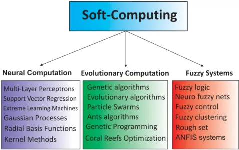
1.2 Soft-Computing sub-branches, including Neural Computation and Learning
Sys-tems, Evolutionary Computation and Fuzzy Systems. . . 3
1.3 An scheme of Artificial Neural Network model. . . 4
1.4 Flowchart diagram of the original CRO algorithm. . . 8
1.5 Example of reef in the CRO-SL, where there are five substrate layers associated
with the broadcast spawning process. Each substrate layer represents now a
different exploration process to carry out in that substrate. . . 10
1.6 (a) Outline of a Wrapper method; (b) Outline of a Filter method. . . 11
1.7 AM calculation process. From a selection of measuring points to be evaluated
(marked in red), the AM approach works by calculating the field reconstruction error for all the evaluation period, by looking for the most similar situation in the training period, considering only the information provided by the selected
measuring points. . . 15
2.1 Wikinger wind farm (North sea); (a) Wind farm contour and possible location
points; (b) Best solution obtained with an EA; (c) Best solution obtained with
the CRO approach. . . 28
2.2 Evolution comparison between the CRO-SP and CRO-SL in the problem of energy
prediction from macro-economic variables in Spain; (a) CRO-SP; (b) CRO-SL. . 32
2.3 Evolution of the number of corals within generations (CRO-SP) in the problem
of energy prediction from macro-economic variables in Spain. . . 33
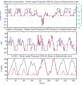
2.4 Comparison of the results obtained using the proposed CRO-SL (blue line) and the
deterministic approach (red line) for a winter week in the micro-grid considered; (a) Consumption from the main grid, (b) Battery power scheduling and (c)%
SOC (State of Charge) in the battery. . . 33
2.5 Comparison of the effect of the different substrates of the CRO-SL in the Winter
week considered (percentage of times in which a given substrate gives the best
larva (new solution) in each generation). . . 34
3.2 Example of the grid and measuring tower in a wind farm. . . 39
3.3 Location of the wind farm considered to test the CRO-ELM algorithm. . . 40
3.4 Best CRO-ELM and CRO-LR evolution (see text for details); (a) CRO-ELM; (b)
CRO-LR. . . 43
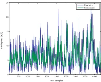
3.5 Wind speed prediction obtained with the CRO-ELM algorithm and real wind speed. 43
3.6 Wind farm considered for the experiments in the CRO-SL-ELM case. . . 45
3.7 Scatter plots of the wind speed hourly estimation by the ELM method for the
test data set: (a) without feature selection; (b) with CRO-SL for the selection. . 51
3.8 Temporal evolution of the wind speed hourly estimation by the ELM method for
the test data set: (a) without feature selection; (b) with CRO-SL for the selection. 51
4.1 GSR prediction scheme used. . . 56
4.2 Location of: (a) Toledo’s measuring station in Spain and (b) the M = 2 WRF
grid points considered for the downscaling . . . 57
4.3 Scatter plot of the global solar radiation: (a) Experiment E1, (b) Experiment E2
and (c) ExperimentE3. . . 61
4.4 Experiment E3. (a) GSR over time. (b) Deviation in time of the predicted GSR
from the measured GSR. Note that only a random time frame of 100 samples is
presented for clarity purposes. . . 62
4.5 ExperimentE3. Evolution with the number of iterations of the best coral’s RMSE.
Note that the best coral belongs to speciesS2. . . 62
4.6 ExperimentE3. Evolution of the species present in the reef after a certain number
of iterations (k): (a) k = 1; (b) k = 10; (c) k = 25; (d) k = 50; (e) k = 150.
Each color pixel stands for a different coral species and free cells in the reef (free
(black),S1 (magenta),S2 (blue), S3 (green),S4 (red) and S5 (cyan)). . . 63
4.7 Experiment E1. Evolution with the number of iterations of: (a) The RMSE of
each species’ best coral, and (b) The number of corals per species. . . 63
4.8 Experiment E2. Evolution with the number of iterations of: (a) The RMSE of
each species’ best coral, and (b) The number of corals per species. . . 64
4.9 Experiment E3. Evolution with the number of iterations of: (a) The RMSE of
each species’ best coral, and (b) The number of corals per species. . . 64
5.1 An example of the integer encoding of solutions chosen for the RS problem at
hand in the CRO-SL. . . 69
5.2 Location of measuring stations (ECA) and reanalysis points (ERA); (a) Measuring
stations of ECA and HISTALP dataset (un-grided measuring stations) for the first temperature RS problem considered; (b) Location of the ERA-Interim reanalysis
5.3 RMSE landscape in the ECA dataset, for all combinations (pairs) of measuring
stations (special case N = 2); (a) Landscape (3D); (b) Contour plot (2D). . . 72
5.4 RMSE landscape in the ERA dataset, for all combinations (pairs) of measuring
stations (special case N = 2); (a) Landscape (3D); (b) Contour plot (2D). . . 73
5.5 Best representative station (caseN = 1) for the ECA dataset and greedy approach
construction; (a) Reconstruction error for (N = 1); (b) Greedy (construction
based) solution obtained for the caseN = 10. . . 73
5.6 Best solution found by the CRO-SL (red points stand for the selected
represen-tative measuring stations), for the ECA dataset; (a) N = 5; (b) N = 10; (c)
N = 15 and (d)N = 20. . . 76
5.7 Best solution found by the CRO-SL (red points stand for the selected
represen-tative nodes), for the ERA dataset; (a) N = 5; (b) N = 10; (c) N = 15 and (d)
N = 20. . . 77
5.8 Best solution found (red points) by the CRO-SL, for the ECA dataset (hindcasting
problem); (a) N = 5; (b)N = 10; (c)N = 15 and (d) N = 20. . . 79
5.9 Best solution found (red points) by the CRO-SL, for the ERA dataset (hindcasting
problem); (a) N = 5; (b)N = 10; (c)N = 15 and (d) N = 20. . . 80
5.10 Set of least representative stations (red points) as inferred by the CRO-SL for
N = 10 in ECA (a) and ERA (b) datasets. . . 81
5.11 Reconstruction RMSE ◦C per station/node in the test period (e(sk,s10) =
q
1
tV PtV
T=1(F(sk, T∗)−F(sk, T))2), in ECA and ERA datasets (N = 10 case). . 81
5.12 Reconstruction error (F(s∗, T∗)−F(s∗, t)) in ECA and ERA datasets (best station
(s∗), N = 10 case); (a) ECA dataset; (b) ERA dataset. . . 82
5.13 Real and reconstructed (AM method) temperature in the best station (N = 10
case) for the ECA abd ERA dataset (complete test period and zoom in the last
two years); (a) ECA dataset; (b) ERA dataset. . . 83
5.14 Best solution found (red points) by the CRO-SL, for the ERA dataset with
dif-ferent temporal scale (N = 5); (a) daily; (b) Monthly; (c) Quarterly and (d)
Annual. . . 85
5.15 Best solution found (red points) by the CRO-SL, for the ERA dataset with
dif-ferent temporal scale (N = 10); (a) daily; (b) Monthly; (c) Quarterly and (d)
Annual. . . 86
5.16 Best solution found (red points) by the CRO-SL, for the ERA dataset with
dif-ferent temporal scale (N = 15); (a) daily; (b) Monthly; (c) Quarterly and (d)
Annual. . . 87
5.17 Best solution found (red points) by the CRO-SL, for the ERA dataset with
dif-ferent temporal scale (N = 20); (a) daily; (b) Monthly; (c) Quarterly and (d)
for the ECA and ERA datasets in the caseN = 10; (a) Number of new larvae in the reef (ECA); (b) Percentage of best larvae formed (ECA); (c) Number of new
larvae in the reef (ERA); (d) Percentage of best larvae formed (ERA). . . 89
6.1 Location of the measuring points in the ERA-Interim reanalysis nodes considered. 92
6.2 RMSE (m/s) obtained with the CRO-SL approach for different values of N. . . . 95
6.3 Best solution found by the CRO-SL (red points stand for the selected
represen-tative nodes); (a) N = 5; (b) N = 10; (c) N = 15 and (d)N = 20. . . 96
6.4 Reconstruction error of the wind speed field (normalized by the average wind
speed of each point) with the Analogue method, for different number of selected
representative points; (a)N = 5; (b) N = 10; (c)N = 15 and (d)N = 20. . . 97
6.5 Reconstruction error for the best measuring point reconstructed with the
Ana-logue method, for different number of selected representative points; (a) N = 5;
(b)N = 10; (c)N = 15 and (d) N = 20. . . 98
6.6 Best solution found by the CRO-SL (20 representative points), in different seasons;
(a) Spring; (b) Summer (c) Autumn and (d) Winter. . . 99
6.7 Least representative points for the wind speed field reconstruction; (a) N = 5;
(b)N = 10; (c)N = 15 and (d) N = 20. . . 100
6.8 Percentage of best larvae obtained in the CRO-SL from each substrate, in the
case N = 20. . . 101
6.9 Evolution of the number of new larvae in the CRO-SL which are able to get into
List of Tables
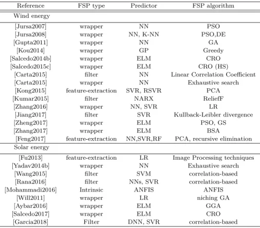
2.1 Summary of the most important articles applying feature selection methods in
energy applications. . . 26
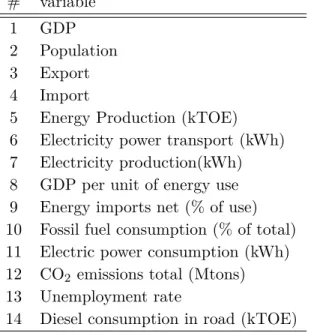
2.2 Variables considered in the problem of energy demand estimation at a nation level. 29
3.1 Predictive meteorological variables used in the short-term wind speed prediction
problem considered. . . 41
3.2 Results obtained with the CRO-ELM and EA-ELM in the FSP problem associated
with short-term wind speed prediction. . . 42
3.3 Results obtained (RMSE in m/s) with the ELM and SVR approaches as prediction
algorithms, using the features selected by the CRO-ELM and CRO-LR algorithms. 44
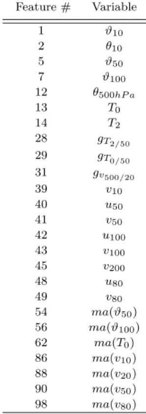
3.4 Complete set of predictive features from the WRF model for wind speed prediction. 47
3.5 Results of the hourly and daily wind speed estimation by the ELM and MLR
with all features considered (98). . . 48
3.6 Comparative best results of the hourly wind speed prediction by the ELM and
MLR, with different fitness functions in the CRO and CRO-SL algorithms. . . . 48
3.7 Best set of features selected by the CRO-SL (f1(x), 25 features). . . 49
3.8 Comparative best results of the daily wind speed estimation by the ELM and
MLR, with different fitness in the CRO-ELM and CRO-SL-ELM algorithm. . . . 50
3.9 Comparative best results of the hourly wind speed estimation by a SVR and
MLP regressors, with all features, CRO-ELM and CRO-SL-ELM, considering
fitness functionf1. . . 50
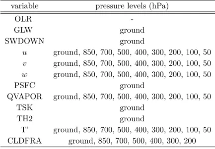
4.1 Outputs of the WRF model used in the experiments as predictive variables (58
variables per point of the WRF model). . . 59
4.2 CRO-SP optimization parameters. . . 60
4.3 Experiments run considering different species. Each speciesis represented bySi. 60
4.4 Best predictive variables found for each experiment. Those variables present in
all three experiments’ results have been highlighted in bold face. . . 65
4.5 Comparison of the results obtained with other metaheuristic techniques. . . 65
5.1 CRO-SL optimization parameters. . . 74
5.3 Results in terms of the RMSE for the field reconstruction (◦C) obtained in ECA and ERA datasets (hindcasting problem), by the CRO-SL, HS, DE, Hill Climbing
and greedy approaches. . . 78
6.1 Parameters of the optimization meta-heuristics compared in this paper: CRO-SL,
HS, EA, PSO and SA. . . 93
6.2 Results in terms of the RMSE for the wind speed field reconstruction (m/s)
obtained in the Europe reanalysis data, by the CRO-SL, HS, EA, PSO and SA
2Px 2-points crossover
AFWA Air Force Weather Agency (USA)
AI Artificial Intelligence
AM Analogue Method
ANFIS Adaptive Neuro-fuzzy Inference System
ANN Artificial Neural Network
AO Antarctic Oscilation
ARMA Auto-Regressive Moving Average model
ARIMA Auto-Regressive Integrated Moving Average model
BSA Backtracking Search Algorithm
CNN Convolutional Neural Networks
CRO Coral Reefs Optimization algorithm
CRO-SL Coral Reefs Optimization with Substrate Layer algorithm
CRO-SP Coral Reefs Optimization with Species algorithm
DECRO Differential Evolution Coral Reefs Optimization algorithm
DNN Deep Neural Network
DE Differential Evolution
EA Evolutionary Algorithm
ECMWF European Centre for Medium-Range Weather Forecasts
ELM Extreme Learning Machine
EMD Empirical Mode Decomposition
ENSO El Niño/Southern Oscilation
FAA Federal Aviation Administration (USA)
FSL Forecast Systems Laboratory (USA)
FSP Feature Selection Problem
GA Genetic Algorithm
GFS Global Forecasting System
GGA Grouping Genetic Algorithm
GP Gaussian Process
GS Gravitational Search algorithm
GSR Global Solar Radiation
GHI Global Horizontal Irradiance
HS Harmony Search
k-NN k-Nearest Neighbors
LA-CRO Learning Automata Coral Reefs Optimization algorithm
LR Linear Regression
MASL Metres Above Sea Level
MCP Measure Correlate Predict approaches
MERRA Modern-Era Retrospective analysis for Research and Applications
ML Machine Learning
MLP Multi-Layer Perceptrons
MPx Multi-points crossover
MLR Multi-Linear Regression
MSE Mean Squared Error
MSVR Multi-output Support Vector Regression
NARX Nonlinear Auto-Regressive eXogenous model
NCAR National Center for Atmospheric Research (USA)
NCEP National Center for Environmental Prediction (USA)
NDBC National Data Buoy Center of the USA
NN Neural Network
NOAA National Oceanic and Atmospheric Administration (USA)
NWP Numerical Weather Prediction models
NC Neural Computation
PAR Pitch Adjusting Rate
PCA Principal Component Analysis
PSO Particle Swarm Optimization
PV Photo-Voltaic sytems
RBF Radial Basis Function networks
RE Renewable Energy
RF Random Forest
RMSE Root Mean Square Error
RS Representative Selection
RSVR Reduced Support Vector Regression
SA Simulated Annealing
SM Standard integer Mutation
SURFRAD NOAA Surface Radiation Network (USA)
SVM Support Vector Machine
SVR Support Vector Regression
TOE Tons Oil Equivalent
WEKA Waikato Environment for Knowledge Analysis
Chapter 1
Introduction
1.1
Motivation and objective
In the last decade, global energy demand has increased to non-previously seen levels, pushed by the increase in global population, fierce urbanization in developed countries and aggressive industrial development all around the world [Suganthi2012]. Conventional fossil-based energy sources have limited reservoirs and a deep environmental impact (contributing to global warm-ing) [Bauer2015], and therefore they cannot satisfy this global demand for energy in a sustainable way [Rowland2016]. These issues related to fossil-based sources have led to a very important development of RE sources in the last years, mainly in renewable technologies such as wind or solar-based. The main problem with RE resources is their dependency on meteorological conditions, sometimes extreme, such as in the case of wind and solar energy [Kumar2016]. The fact that individual renewable sources cannot provide continuous power supply because of their uncertainty and intermittent nature is also an important issue which must be solved to improve the penetration of these resources in the electric system. Note that nowadays renewable energy resources cover approximately 19% of the total World energy demand [REN21-2017] (see Figure 1.1). This figure is still far from the non-renewable sources, which are estimated to cover almost 78% of the total demand, specially in developing countries. A huge amount of research is being conducted to obtain a higher penetration of renewable resources into the electric system.
Currently, the development of Information Technologies has led to a new era in
computa-tion, mainly ruled byData Science. Data science and related technologies are nowadays of major
importance in our society, since they play the highest roles in the development of a global, fully-connected, economy. In this regard, Soft-Computing and its related paradigms (Machine Lear-ning, Computational Intelligence, etc.) have proven to be excellent tools to cope with difficult problems arisen in Data Science, in a huge variety of applications such as Medicine [Bisaso2017], Manufacturing [Sharp2018] or social networks [Bello2016], among many others. In this sense, Soft-Computing techniques have also been successfully applied to RE and atmospheric-related problems [Gardner1998, Renani2016, Kalogirou2006, Heinermann2016, Jha2017, Voyant2017,
78.3%
Fossil Fuels
19.2%
All Renewables
Nuclear
2.5%
Figure 1.1: Implantation percentage of Renewables, Fossil Fuels and Nuclear energy at global level by 2016 [REN21-2017].
Sharma2018].
Soft-Computing is a branch of AI whose objective is to obtain robust problem solving tech-niques which emulate the human thinking. It is a huge research area, which merges different paradigms and lines of research including statistical learning, neural and cognitive signal pro-cessing, natural computing or fuzzy logic, among others. Moreover, Soft-Computing is a live research field, where new approaches are proposed for dealing with very hard problems which arise every day in Engineering and Science. Figure 1.2 shows a scheme of Soft-Computing which includes a first classification of techniques, such as Neural Computation and Learning Systems, dealing with regression and classification problems, or any type of supervised prediction pro-blem, Evolutionary computation, a wide area which includes natural computing approaches, mainly devoted to optimization problems and systems, and finally Fuzzy systems, a line more linked with robotics and control systems.
This Ph.D. Thesis discusses new hybrid Soft-Computing approaches to solve problems re-lated to RE and atmospheric science. We explore new approaches that merge a new type of Evolutionary Algorithm (the CRO algorithm), in different versions, with some kind of predic-tion or reconstrucpredic-tion approaches, such as NNs or the AM. The motivapredic-tion of this work is the necessity for obtaining new powerful approaches which lead to better solutions in difficult problems (those that cannot be properly solved with traditional methods). The application of Soft-Computing techniques is fully justified in these cases, offering an alternative which is cur-rently being exploited by many researchers and practitioners, with paradigms such as Big Data or Deep Learning [LeCun2015]. In this sense, hybrid approaches mixing Soft-Computing with alternative ML algorithms or methods is a line followed in the last years by many researchers [Tasci2014].
1.2. Soft-Computing algorithms and methods used 3
Soft-Computing
Evolutionary Computation Fuzzy Systems
Fuzzy logic Neuro fuzzy nets Fuzzy control Fuzzy clustering Rough set Multi-Layer Perceptrons
Support Vector Regression
Extreme Learning Machines
Gaussian Processes Radial Basis Functions Kernel Methods Genetic algorithms Evolutionary algorithms Particle Swarms Ants algorithms Genetic Programming Coral Reefs Optimization
Neural Computation
ANFIS systems
Figure 1.2: Soft-Computing sub-branches, including Neural Computation and Learning Systems, Evolutionary Computation and Fuzzy Systems.
proposed and alternative methods applied. At the end of the chapter, the structure of the rest of this Thesis will be discussed, where the main algorithms proposed and problems tackled are outlined.
1.2
Soft-Computing algorithms and methods used
1.2.1 Neural Computation-based approaches
Neural Computation is a part of Soft-Computing that includes algorithms inspired on how the human brain learns. It is based on algorithms usually known as ANNs. Neural Compu-tation includes a large amount of different NNs, which have been mainly used in classification
and regression problems. In this work, we consider feed forward neural networks, a type of
neural processing approach which processes the information in different layers, with a privileged direction. MLPs are the most used feed forward neural approaches, and will be described next, together with ELMs, a kind of feed forward network with a very fast training scheme, perfect for constructing hybrid algorithms.
Multi-layer perceptrons
A MLP is a particular kind of ANN which is massively parallel. It is considered a distributed information-processing system, which has been successfully applied in modelling a large variety of nonlinear problems [Haykin1998, Bishop1995]. The MLP consists of an input layer, a number of hidden layers, and an output layer, all of which are basically composed by a number of special
processing units called neurons, as Figure 1.3 shows. As important as the processing units themselves is their connectivity, i.e. how the neurons within a given layer are connected to those of other layers by means of weighted links. These weight values are closely related to the learning ability of the MLP, and also with its ability to generalize the learning from enough number of
examples. Thus, note that such a learning process demands a proper database containing
a variety of input examples or patterns with the corresponding known outputs (tags). The adequate values of the neuron weights minimize the error between the output generated by the MLP (when fed with input patterns in the database), and the corresponding expected output in the database. The number of neurons in the hidden layer is a parameter to be optimized when using this type of neural network [Haykin1998, Bishop1995].
Figure 1.3: An scheme of Artificial Neural Network model.
The input data for the MLP consists of a number of samples arranged as input vectors,
x={x1, . . . , xN}. Once a MLP has been properly trained, validated and tested using an input
vector different from those contained in the database, it is able to generate a proper output y.
The relationship between the output and the input signals of a neuron is the following:
y=ϕ n X j=1 wjxj −θ , (1.1)
wherey is the output signal,xj forj= 1, . . . , nare the input signals,wj is the weight associated
with the j-th input, and θis a threshold [Haykin1998, Bishop1995]. The transfer function ϕis
usually considered as the logistic function,
ϕ(x) = 1
1 +e−x. (1.2)
The process to obtain an accurate output is related to the training procedure as it was mentioned before. During the training process, the error between the estimated output and its
1.2. Soft-Computing algorithms and methods used 5
corresponding real value in the database will determine to what degree the weights in the network should be adjusted. Hence, the objective of the network training is to find the combination of weights which results in the smallest training error with the best possible generalization of the result. There are different algorithms that can be used to train a MLP. One possible technique is the back-propagation training algorithm [Bishop1995] which uses the procedure known as
gradient descent to try to locate the global minimum of the error [Gardner1998]. Another approach is the well-known Levenberg-Marquardt [Hagan1994].
Extreme Learning Machine
An ELM [Huang2015, Huang2006] is a novel and fast training method based on the structure of MLPs, shown in Figure 1.3. The most significant characteristic of the ELM training is that it is carried out just by randomly setting the network weights, and then obtaining a pseudo-inverse of the hidden-layer output matrix. The advantages of this technique are its simplicity, which makes the training algorithm extremely fast, and also its outstanding performance when compared to alternative sequential learning methods, usually better than other established approaches such as classical MLPs. Moreover, the universal approximation capability of the ELM network, as well as its classification capability, have been already proven [Huang2012].
The ELM algorithm can be summarized as follows: given a training set T =
(xi,yi)|xi∈Rn,yi∈R, i= 1,· · ·, l, an activation function g(x), which a sigmoidal function is
usually used, and number of hidden nodes ( ˜N),
1. Randomly assign inputs weights wi and biasbi,i= 1,· · · ,N˜.
2. Calculate the hidden layer output matrix H, defined as
H= g(w1x1+b1) · · · g(wN˜x1+bN˜) .. . · · · ... g(w1xl+b1) · · · g(wN˜xN +bN˜) l×N˜ (1.3)
3. Calculate the output weight vectorβ as
β=H†yt, (1.4)
where H† stands for the Moore-Penrose inverse of matrix H [Huang2006], and yt is the
training output vector,yt= [yt1,· · ·,ytl]T.
Note that the number of hidden nodes ( ˜N) is a free parameter of the ELM training, and
must be estimated for obtaining good results. Usually, scanning a range of ˜N values is the
best solution. The Matlab extreme learning machine implementation by G. B. Huang, freely available at [ELM2018], is often considered for ELM implementation.
1.2.2 The Coral Reefs Optimization Algorithm
The CRO is a novel evolutionary-type meta-heuristic approach for optimization, recently developed in [Salcedo2014d], which is based on simulating the corals’ reproduction and coral reefs’ formation processes. The CRO algorithm tackles optimization problems by modeling and
simulating all the distinct processes in a real coral reef. Let R be a model of reef, consisting
of a N ×M square grid. We assume that each square (i, j) of Ris able to allocate a coral (or
colony of corals) Ξi,j, representing different solutions to our problem, using a given encoding for
the problem at hand (an encoding is a representation of the optimization problem’s variables,
usually in the form of a chain of numbers, leading to a givensearch space). The CRO algorithm is
first initialized at random by assigning some squares inRto be occupied by corals (i.e. solutions
to the problem) and some other squares in the grid to be empty, i.e. holes in the reef where new
corals can freely settle and grow. The rate between free/occupied squares inRat the beginning
of the algorithm is a parameter of the CRO algorithm denoted as ρ, and note that 0< ρ0 <1.
After the reef initialization, a second phase of reproduction and reef formation is carried out. First, a simulation of the corals’ reproduction in the reef is done by sequentially applying different operators for modeling sexual reproduction (broadcast spawning and brooding), asexual reproduction (budding), and polyps depredation:
1. Broadcast Spawning (external sexual reproduction): the modeling of coral
repro-duction by broadcast spawning consists of the following steps:
1.a. In a given stepkof the CRO algorithm, select uniformly at random a fraction of the
existing corals ρk in the reef to be broadcast spawners. The fraction of broadcast
spawners with respect to the overall amount of existing corals in the reef will be
denoted as Fb. Corals that are not selected to be broadcast spawners (i.e. 1−Fb)
will reproduce by brooding later on in the algorithm.
1.b. Select couples out of the pool of broadcast spawner corals in step k. Each of such
couples will form a coral larva by means of a given crossover mechanism or any other exploration strategy. Note that once two corals have been selected to be the parents
of a larva, they are not chosen anymore in step k (i.e. two corals are parents only
once in a given step). This couple selection can be done uniformly at random or by resorting to any fitness proportionate selection approach (e.g. roulette wheel).
2. Brooding (internal sexual reproduction): at each step kof the reef formation phase
in the CRO algorithm, the fraction of corals that will reproduce by brooding is 1−Fb.
The brooding modeling consists of the formation of a coral larva by means of any kind of mutation mechanism, in order to simulate of the brooding-reproductive coral (self-fertilization considering hermaphrodite corals).
1.2. Soft-Computing algorithms and methods used 7
3. Larvae setting: once all the larvae are formed at stepkeither through broadcast spawn-ing (1.) or by broodspawn-ing (2.), they will try to set and grow in the reef. First, the health function (fitness) of each coral larva is computed. Second, each larva will randomly try to
set in a square (i, j) of the reef. If the square is empty (free space in the reef), the coral
grows therein no matter the value of its health function. By contrast, if a coral is already occupying the square at hand, the new larva will set only if its health function is better
than that of the existing coral. We define a numberκ of attempts for a larva to set in the
reef: afterκ unsuccessful tries, it is considered as depredated by the animals in the reef.
4. Asexual reproduction: the modeling of asexual reproduction (budding or fragmenta-tion) is the CRO is carried out in the following way: the overall set of existing corals in
the reef are sorted as a function of their level of health (given by f(Ξij)). Then a small
fractionFaduplicate themselves and are mutated in order to obtain variability. These new
corals try to settle in a different part of the reef by following the setting process described in Step 3.
5. Depredation in polyp phase: corals may die during the reef formation phase of the
CRO algorithm. At the end of each reproduction step k, a small number of corals in
the reef can be depredated, thus liberating space in the reef for next coral generation.
The depredation operator is applied with a very small probabilityPd at each step k, and
exclusively to a fractionFd of the worse health corals in R.
Figure 1.4 illustrates the flowchart diagram of the CRO algorithm, with the different CRO phases (reef initialization and reef formation), along with all the operators described above.
1.2.3 Advanced CRO models
The basic CRO can be improved to obtain stronger versions of the meta-heuristic, based on alternative processes that occur in coral reefs. We describe here two different modifications of the CRO algorithm which improve its performance in specific applications. First, we describe the CRO with species, which helps tackle optimization problems with variable length encodings. It is also useful for managing different encodings of problems within the same population, obtaining a competitive co-evolution algorithm. The second version is the CRO with substrates layer. It has been useful to obtain a competitive co-evolution algorithm in which different models are applied to the same problem. These models can be either exploration models, repairing mechanisms, etc., and the only pre-requisite is that the objective function to evaluate corals in the reef must be the same for the different models considered.
Reef initialization
Coral larvae formation by broadcast spawning Coral larvae formation by brooding
Larvae setting Budding or fragmentation stopping condition fulfilled? yes No Coral predation Finish Re ef forma tion simula tion
Figure 1.4: Flowchart diagram of the original CRO algorithm.
CRO with species
The first modification of the CRO consists in considering different coral species within a single coral community (CRO-SP). The objective of this modification is that each coral species
represents a different model (or its hyper-parameters) out ofT possible models. In this context,
modelis generic, so it can represent either a different encoding for the problem, a different way of calculating the objective function, etc. The CRO-SP is a new powerful way of managing opti-mization problems with variable or different encodings. In this case, each species will represent a different encoding, and the idea is that only corals of the same species can reproduce in the broadcast spawning operator. Note however, that all the models compete together in the larvae setting, since the objective function in all cases should be the same for all the species.
The CRO-SP was first introduced in [Salcedo2017b] as a methodology to deal with a Model
Selection Problem, in an application of total energy consumption prediction in Spain. In
[Salcedo2017b] each species represents a different way of calculating the total energy consump-tion (a different model), and the idea was to build a competitive co-evoluconsump-tion approach that obtained the best possible model in addition to alternative parameters such as the best predic-tion variables to feed the predicpredic-tion model. Note that the CRO-SP could be also used to evolve a competition of different regressions for a given problem, for example neural networks, support vector machines, etc., in which the CRO encodes the parameters of each regressor.
1.2. Soft-Computing algorithms and methods used 9
that the competition among species will produce emerging behavior, so the best model (species) eventually will dominate, and will occupy the majority of spaces in the reef.
Require: Valid values for CRO parameters.
Ensure: The best model out ofT possible.
1: Algorithm initialization (T different species)
2: for each iteration of the CROdo
3: Update values of influential variables: mortality probability and the probability of
asexual reproduction
4: Asexual reproduction (budding or fragmentation)
5: Sexual reproduction 1 (broadcast spawning, only same species can reproduce)
6: Sexual reproduction 2 (brooding, only same species can reproduce)
7: Settlement of new larvae (competition among species)
8: Mortality process
9: Evaluate the new population in the reef (with the specific model given for each species)
10: end for
CRO with Substrate Layers
The second important modification of the CRO is the incorporation of substrate layers (CRO-SL). It is based on the fact that there are many more interactions in real reef ecosystems which can be also modelled and incorporated to the CRO approach to improve it. For example, different studies have shown that successful recruitment in coral reefs (i.e., successful settlement and subsequent survival of larvae) depends on the type of substrate on which they fall after the reproduction process [Vermeij2005]. This specific characteristic of the coral reefs was first included in the CRO in [Salcedo2017b], in order to solve different instances of the Model Type Selection Problem for energy applications. In [Salcedo2016c, Salcedo2017b], different substrate layers were defined in the CRO, in such a way that each layer represents a different model to evaluate the energy demand estimation in Spain, from macro-economic variables.
As in the case of the CRO-SP, the CRO-SL is a very general approach: it can be defined as an algorithm for competitive co-evolution, where each substrate layer represents different processes (different models, operators, parameters, constraints, repairing functions, etc.). The inclusion of substrate layers in the CRO can be done in a straightforward manner: we redefine the artificial
reef considered in the CRO in such a way that each cell of the reefRis now defined by 3 indices
(i, j, t), whereiandjstand for the cell location in the grid, and indext∈T defines the substrate
layer, by indicating which structure (model, operator, parameter, etc.) is associated with the
cell (i, j). Each coral in the reef is then processed in a different way depending on the specific
substrate layer in which it falls after the reproduction process. Note that this modification of the basic algorithm does not imply any change in the corals’ encoding (all the corals in the algorithm are encoded in the same way).
The CRO-SL has been applied in [Salcedo2016c] to obtain a competitive co-evolution al-gorithm in which each substrate is assigned to a different implementation of an exploration procedure. Thus, each coral will be processed in a different way in the reproduction step of the algorithm depending on the substrate it occupies. Figure 1.5 shows an example of the CRO-SL, with different substrate layers. Each one is assigned to a different exploration process, Harmony Search based, Differential Evolution, 1-point crossover or Gaussian mutation (alternative as-signment and different exploration processes can be used in the substrate layer of the CRO-SL approach).
HS DE 1-Point
Crossover Gaussian
mutation 2-PointsCrossover
Figure 1.5: Example of reef in the CRO-SL, where there are five substrate layers associated with the broadcast spawning process. Each substrate layer represents now a different exploration process to carry out in that substrate.
The CRO-SL is a general procedure to co-evolve different models, operators, parameter va-lues, etc., with the only requisite that there is only one health function defined in the algorithm. In other words, each substrate can include a different processing of problem’s constraints, ex-ploration or exploitation procedures etc.
1.3
Feature Selection in Machine Learning
Feature selection is an important task in ML-related problems because irrelevant features, used as part of the training procedure of different prediction systems, can increase the cost and running time of the system, and make its generalization performance much poorer [Blum1997, Weston2000]. In its more general form, the FSP for a learning problem from data can be defined
as follows: given a set of labeled data samples (x1, y1), . . . ,(xl, yl), where xi ∈ Rn and yi ∈R
(or yi ∈ {±1} in the case of classification problems), choose a subset of m features (m < n),
that achieves the lowest error in the prediction of the variableyi.
Thus, note that there are many different algorithms which can be used to solve a FSP. In general, they can be structured in two different families or paradigms:
algo-1.3. Feature Selection in Machine Learning 11
ML classifier/regressor
Feature Selection Algorithm
101101011
Initial data base
Training and test
feature selection 100100011 Final solution (a) Feature Selection Algorithm 101101011
Initial data base
Training and test
100100011
Final solution
feature selection
External measure Mutual Information, etc.
(b)
Figure 1.6: (a) Outline of a Wrapper method; (b) Outline of a Filter method.
part of the evaluating function. Figure 1.6 (a) shows the idea behind the wrapper approach: the classifier/regression technique is run on the training dataset with different subsets of features. The one which produces the lowest estimated error in an independent but rep-resentative test set is chosen as the final feature set. For further reading on wrappers me-thods, the following classical works can be consulted [Kohavi1997, Yang1998, Salcedo2002]. In the case of the wrapper method, the FSP admits a mathematical definition as follows:
The FSP consists of finding the optimum n-column vector σ, where σi ∈ {1,0}, that
defines the subset of selected features, which is found as
σo =arg min σ,α Z V(y, f(x∗σ,α))dP(x, y) , (1.5)
whereV(·,·) is a loss functional, P(x, y) is the unknown probability function the data was
sampled from and we have defined x∗σ = (x1σ1, . . . , xnσn). The functiony=f(x,α) is
the classification/regression engine that is evaluated for each subset selection, σ, and for
each set of its hyper-parameters,α.
• In the filter approach to the FSP, the feature selection is performed based on the data,
ignoring the classifier algorithm. An external measure calculated from the data must be defined to select a subset of features. After the search, the best feature subset is evaluated on the data by means of the classifier/regression algorithm. Note that filter algorithms performance completely depends on the measure selected for comparing sub-sets. Figure 1.6 (b) shows an example of how a filter algorithm works. Filter methods are usually faster than wrapper methods. However, their main drawback is that they totally ignore the effect of the selected feature subset on the performance of the classifica-tion/regression algorithm during the search. So, usually their performance is poorer than wrapper approaches. Further analysis and application of filter methods can be found in [Torkkola2000, Torkkola2002].
• There are different works which have combined both wrapper and filter methodologies
to build hybrid approaches. They have shown good performance in specific applications [Ferreira2014, Huda2014, Huda2016, Solorio2016].
For both wrapper and filter methods, a binary representation can be used for the FSP, where
a 1 in theithposition of the binary vector means that the featureiis considered within the subset
of features, and a 0 in thejthposition means that featurej is not considered within the subset.
Note that using this notation is equivalent to encode the problem as the vector σ included in
expression (1.5). Note also that there are 2n different subsets (where n is the total number
of features), and the problem is to select the best one in terms of a certain measure, which can be either internal (wrapper methods) or external (filter methods) to the classifier/regressor. Alternative encodings, such as integer vectors, are however also possible, and even more adequate in some specific applications.
1.4. Representative measuring points selection 13
1.4
Representative measuring points selection
In ML, a Representative Selection (RS) problem consists of finding exemplar samples from
a given data, points or items collection, in such a way that the selected exemplars accurately summarize the complete set of starting data [Wang2017]. RS problems appear in many differ-ent Science and Engineering problems, such as Computer Science [Wang2017], Bio-mechanics [Katrin2012] or Networking [Poorter2017]. In Climatology, RS problems have been faced in different applications, such as dynamical climate downscaling [Rife2013], selecting regional cli-mate scenarios [Wilcke2016], selecting the most representative subset of global clicli-mate models in terms of a given error measure [Ruane2017], selecting the most representative models for climate change studies [Lutz2016], or optimizing the position of weather monitoring stations [Amorim2012].
Let F(s, t) be a field of a climatological variable, defined in a set of |S|measuring points or
stations s, during an observation period ˆt. Such period can be split into a training period, tT,
and a validation or test period of duration tV, in such a way that ˆt=tT +tV. Letχ be a given
reconstruction algorithm for the field F(s, t). χ operates in a subset of measuring stationssN,
where N (N <|S|) represents the number of measuring points or stations selected. Moreover,
note that χ only uses the data in the training period to obtain the best reconstruction of the
initial field F(s, t), in terms of an error measure e(sN) evaluated in the test period. The RS
problem we face in this Thesis consists of obtaining the best possible subset of N measuring
pointss∗N, which minimizese(s∗N) (usuallyestands for a mean square or absolute error function).
Note that the subset s∗N stands for the N most representative measuring stations for the field
F(s, t), in terms of the reconstruction algorithm χ considered. We have chosen the well-known
Analogue Method as the reconstruction algorithm χ.
The Analogue Method in RS
The AM is a prediction/reconstruction algorithm very used in atmospheric sciences. It is based on the principle that two similar states of the atmosphere lead to similar local effects [Lorentz1969]. More specifically, two states of the atmosphere are considered as “analogues”, when there is a resemblance between them, in terms of an analogy criterion and objective variables. Thus, the AM consists of searching for a certain number of past situations in a meteorological archive, in such a way that they present similar properties to that of a target situation for any chosen predictors or variables.
Different versions of the AM can be found in the literature, with a wide range of
mete-orological and climatological applications. In [Gibergans2007] the AM method is improved
by using local thermodynamic data to predict autumn precipitation in Catalonia, Spain. In [Chardon2014], the AM was applied to downscale precipitation in France, including the novelty of spatial similarity in the algorithm. In [DMonache2011] the AM was improved with a Kalman filter in order to improve numerical weather predictions. In [Yiou2014] the AM was applied to a palaeo-climatic problem, specifically, the meteorological reconstruction using circulation
ana-logues in the late Eighteen Century. In [Lguensat2017] the analog data assimilation technique was presented. It combines the AM with ML techniques based on the k-NN to obtain the most important data to be assimilated for numerical prediction systems. AM ensembles have also been applied to different forecasting problems. One of the original works proposing AM en-sembles is [DMonache2013], where the method and its main characteristics have been presented and compared to alternative state-of-the-art numerical weather prediction ensemble systems. In [Junk2015] the statistics of the AM ensemble model are fully described. The AM ensemble has also been applied to specific prediction problems, such as in [Alessandrini2015], where an analog ensemble has been applied to probabilistic solar power forecast in three solar farms in Italy. A comparison with a quantile regression algorithm and persistence ensembles has proven the goodness of the AM approach in this problem. Another work dealing with AM ensembles is [Alessandrini2015b], with application to short-term wind power prediction. In this case the AM ensemble has been applied to the wind power production prediction of a wind farm in northern Sicily (Italy), comparing the performance with alternative algorithms such as quantile regression and numerical weather models. In [Vanvyve2015] another AM ensemble approach is presented, with application in wind resource estimation. The paper analyzes the wind resource of different locations in Europe and USA by applying an AM ensemble.
Finally, note that very recently the AM has been mixed with meta-heuristics algorithms. In [Horton2017] a genetic algorithm has been used to tune the parameters of an AM. The accuracy of this evolutionary-AM approach has been shown in a case study of probabilistic precipitation forecast in Switzerland.
In this Thesis we apply the AM to the RS problem, as follows: Given a subset of measuring
points of stationssN, the AM process starts by obtaining the most similar situations in the past
for the fieldF(sN, tV) (considering all the evaluation period). In other words, this is equivalent
to, for each time T ∈ tV, obtaining the most similar situation (or average of k most similar
situations) in the past (training period), located in time T∗ ∈tT, considering only the selected
measuring points sN (note that T∗ depends on the T considered, i.e. T∗ =T∗(T)). Then, the
complete reconstruction of the fieldF is calculated by using the past situationF(s, T∗) and the
objective situation F(s, T), and a reconstruction error is obtained. The final functione(sN) is
calculated as the root mean square error (RMSE) in the field reconstruction:
e(sN) = v u u u t 1 |S| ·tV tV X T=1 |S| X k=1 (F(sk, T∗)−F(sk, T))2 (1.6)
Figure 1.7 graphically shows the process for the AM application (χ field reconstruction
1.5. Structure of the Thesis 15
Encoded solution
Training period Evaluation period
t=1 t=t t=t
t=T Most similar situation (t=T*)
Reconstruction Error (with all nodes)
e(x)
t=1 T V
(x=SN)
Figure 1.7: AM calculation process. From a selection of measuring points to be evaluated (marked in red), the AM approach works by calculating the field reconstruction error for all the evaluation period, by looking for the most similar situation in the training period, considering only the information provided by the selected measuring points.
1.5
Structure of the Thesis
The rest of this Thesis is organized in a state-of-the-art chapter, where previous works related to the Thesis content are reviewed and analyzed, and two different technical parts:
1. First, contributions with results in RE-related problems are described, which include new hybrid algorithms involving different CRO versions and ELM for problems of feature se-lection in wind and solar resource prediction problems.
2. Second, results in two different RS problems are discussed: optimal measuring points selection for Temperature and Wind fields reconstruction with a hybrid CRO-SL algorithm and the AM reconstruction approach.
To conclude, some final remarks and future research lines are summarized in the last part of the document, with a list of publications produced by the research carried out in this Thesis
Chapter 2
Methods and algorithms: Previous
work
This section presents a description of the state-of-the-art in the technological fields addressed in this Thesis. The idea of this chapter is to focus on the discussion of previous works dealing with the techniques applied in the Thesis.. First, a review of Feature Selection in renewable energy systems is carried out. Wind and solar resources short-term forecasting are first consi-dered, though references in other energy-related problems have also been reviewed. A review of literature devoted to long-term wind speed variability is then discussed. The section is closed with a review of previous work dealing with the CRO algorithm and its variants, with special focus on the results of the algorithm in renewable energy problems.
2.1
A review of FSP methods in renewable energy prediction
problems
This section presents a review of the main works dealing with FSP in renewable energy prediction problems. The section is structured in FSP in wind energy, FSP in solar energy and FSP in energy-related problems.
2.1.1 Feature selection in wind energy prediction systems
Wind energy is the most developed renewable energy technology, and, thus, research on its prediction has been carried out during more than 20 years. FSPs have also been tackled in wind energy during more than a decade. For example, Jursa in [Jursa2007], first proposed a feature selection in wind power prediction systems. Specifically, a PSO approach was introduced in order to obtain the optimal set of features which provided the best prediction. That work was further completed in another paper by Jursa and Rohrig, [Jursa2008], where NN and k-NN algorithms were used as prediction models, and two wrapper feature selection models were