ABSTRACT
The first deep imaging of the southern Appalachians has revealed a double Moho from the Blue Ridge Escarpment towards the North Carolina Piedmont, raising questions of what material is convoluting the crust-mantle boundary (Wagner et al. 2012). We’re presenting work that seeks to test if an eclogite root situated between 40 and 60km depth is permitted with the Bouguer gravity anomaly in this region. Results from this gravity modeling show that two
profiles from Tennessee to North Carolina and from West Virginia to Virginia can include such a root, although small adjustments can be made to support a model without eclogite. We favor the eclogite models over the latter due to their ability to explain the seismic discontinuity found in Wagner et al. (2012) and the density anomaly found in Mooney and Kaban (2010).
INTRODUCTION
Previous tomography in the southern Appalachians by Wagner et al. (2012) reveals a deviation in the expected Mohorovičić (Moho) discontinuity (Figure 1). The authors concluded that an eclogite slab could explain the discontinuity observed in this area due to its density and its associated geologic story. The two current models for the deep structure of the Appalachians that came from this study show a complicated architecture with differing interpretations of how the continental plates merged together. A map of the region published by GSA (1991) also provides several suggested models for the crust and upper mantle in its cross-sections along this transect. In addition to these interpretations, gravity modelling of North America by Mooney and Kaban (2010) has revealed an unexplained density anomaly underneath the southern
Figure 1. Proposed cross-section A – A’ given in Wagner et al. (2012). The doubled Moho can be seen at the base of the Grenville eclogitic root.
These studies have all shown hypothesized structures at the Moho, but no work has been done yet to test if an eclogite root is consistent with the gravity anomaly in the area. This study seeks to improve these models by building crustal and mantle structures to match the Bouguer gravity anomaly profiles along two different transects of the southern Appalachians. Testing these models by looking at their generated gravity profiles will show if a large eclogite slab can exist between 40 and 60 km depth or if a homogenous mantle can fully explain the regional gravity anomaly.
GEOLOGIC SETTING
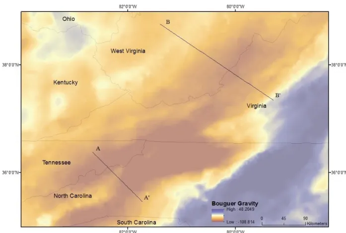
This study looks at the gravity along two different transects across the southern
Cross-section A is the transect that Wagner et al. (2012) imaged the double Moho down to 60km depth, distinguishing this as the location of a possible eclogite root.
During the Appalachian orogeny, the closing of the Iapetus Ocean trapped a subducting oceanic plate underneath Laurentia. While descending, this oceanic slab would experience greater pressures and temperatures to partially eclogitize it, possibly confining it under the existing Grenville basement rocks. At a depth of 60km, the eclogite would have a density of approximately 3.35g/cm3 (Groppo and Castelli 2010). If this did not happen, the plate would have continued descending deeper into the mantle and wouldn’t have much of an effect on the gravity profiles.
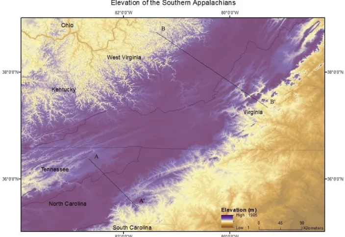
Figure 3. Relatively higher elevation in the southern Appalachians exist where the crust is thinner, which can’t be explained with traditional isostatic compensation models if the crust is homogenous down to 60km.
METHODS
I looked at the general shape of the gravity profiles in this area since that was more informative to the deep structure than seeking to explain every small-wavelength deviation in the profile. Kaban (2010) showed that generalized interpretations of the upper crust are adequate to image deeper structures, but the largest sources of error in this study likely come from an inability to determine precise locations of the different rock units and their corresponding densities. Even small (<0.05g/cm3) changes in a rock unit’s density can substantially alter the experimental gravity curve in that area. Using densities close to the average crustal density of 2.67g/cm3 with informed nonconformities to that average minimized this error. The Carolinia interpretation of the basement rock as explained in Wagner (2012) was used in cross-section A – A’ to illustrate this region’s gravity profile as it was the favored explanation of the tectonic history. Models with a consistent 2.73g/cm3, a lateral extension of the interpreted density for the Grenville basement, also supported the presence of eclogite.
Kaban et al. (2010) cautions that even with ideal data coverage, the standard deviations of residual gravity sources can be over 30mGal. This could substantially impact the accuracy of models where the amplitude of the profiles is small, such as in this field area (50-60mGal). Keeping a consistent upper-crustal structure between the various models helps to mitigate these errors, especially since they would likely be a shorter wavelength than we are interested in here.
See Appendix A for step-by-step instructions to replicate this study.
RESULTS
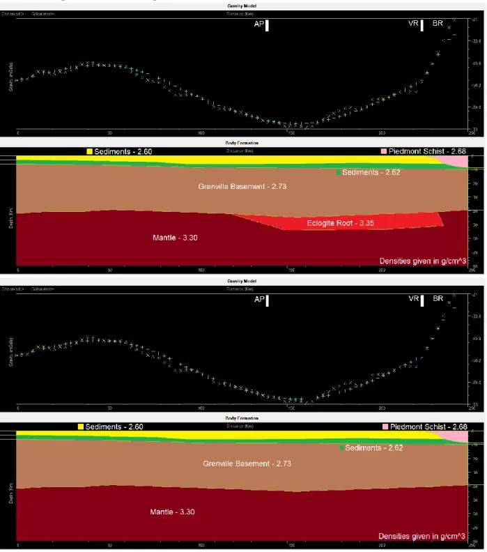
mantle in the area by raising the Moho less than a kilometer. The high density contrast between the crust and mantle compared to the low density contrast between the mantle and eclogite means that the Moho location has much more influence on the gravity signature.
et al. (2012) and Mooney and Kaban (2010). The lower model shows that we can match the gravity profile without an eclogite root. The depth of the Moho near A’ was changed less than a kilometer to provide the lower profile.
We tested these models by replacing the eclogite root with mantle to see how difficult it was to explain the Bouguer gravity in the area. Adjusting the Moho upward by less than a kilometer allows the relatively dense mantle material to displace the lighter crustal material, providing sufficient gravitational pull to match the observed gravity. This illustrates that the Bouguer gravity anomaly does not provide a unique solution to the regional gravity.
DISCUSSION
Figure 6. Taken from Mooney and Kaban (2010), this density anomaly map shows the location of a 0.04 to 0.06 g/cm3 density increase underneath the southern Appalachians.
In addition to the geophysical evidence, an eclogite root would help to explain the regional isostatic compensation. The additional dense material wedged together with the lower crust would pull down on the rest of the plate, significantly lowering the surface elevation. The thinner crust towards A has no such root in these models, and it follows that this lack of dense material pulling it down corresponds to a higher elevation.
CONCLUSION
results of Wagner et al. (2012) and Mooney and Kaban (2010) and the isostatic compensation of the area, we have good evidence to believe that this eclogite root exists at 40 to 60km depth along strike of the Appalachians. The Bouguer gravity profiles could support interpretations of a homogenous mantle on their own, but they would not be able to explain the other phenomena mentioned above.
REFERENCES CITED
Aldouri, R, 2003. Gravity Database of the US, accessed Nov. 7, 2013, available at <http://research.utep.edu/default.aspx?tabid=37229>.
Geological Society of America, 1991. Central Kentucky to the Carolina Trough [map]. Decade of North American Geology Project, Map G 3301 C55 SVAR G4 No. 16. Sheet 1. Scale 1:500,000.
Groppo, C., and Castelli, D., 2010. Prograde P-T evolution of a lawsonite eclogite from the Monviso meta-ophiolite (Western Alps): Dehydration and redox reactions during subduction of oceanic FeTi-oxide gabbro, Journal of Petrology, vol. 51, no. 12: 2489-2514.
Kaban, M.K., Tesauro, M., Cloetingh, S., 2010. An integrated gravity model for Europe’s crust and upper mantle. Earth and Planetary Science Letters, vol. 296: 195-209.
King, E.R., Daniels, D.L., Hanna, W.F., Snyder, S.L., 1998. Magnetic and gravity anomaly maps of West Virginia [map]. U.S. Geological Survey Miscellaneous Investigations Series, Map I-2364-H. Sheet 2. Scale 1:1,000,000.
Mooney, W. D., and M. K. Kaban, 2010. The North American upper mantle: Density,
composition, and evolution, J. Geophys. Res., 115, B12424, doi:10.1029/2010JB000866. Wagner, Lara S., Stewart, Kevin, Metcalf, Kathryn, 2012. Crustal-scale shortening structures
Wilson, Thomas H., 2010. Seismic evaluation of differential tectonic subsidence, compaction, and loading in an interior basin. The American Association of Petroleum Geologists, vol 84, no. 3: 376-398.
This research was funded by a Summer Undergraduate Research Fellowship from the Office for Undergraduate Research at the University of North Carolina at Chapel Hill.
APPENDIX A
Gravity Modeling How-To Programs needed, with recommended version:
ArcGIS 10.1 (Through school) R 3.0.3 (http://www.r-project.org/)
Talwani 2.2 (http://research.utep.edu/Default.aspx?tabid=45290) Notepad ++ 6.5 (http://notepad-plus-plus.org/)
1. Go to the “new application” for downloading gravity and magnetic data here: http://research.utep.edu/default.aspx?tabid=37229
-Download up to 150,000 points at a time. You can download about 8 states’ worth of gravity data at a time.
2. Open the gravity data with excel
-copy the nad83 lat and lon columns, as well as the Bouguer anomaly column -open a new Excel document, fill the first three columns with all the data like this:
Lon Lat Bouguer
83.873219 36.83273 -47.39
-save as .csv 3. Open ArcMap
-Connect to the folder with this file in it -File>Add Data>Add X Y Data
-Lon and Lat should be filled out automatically, select Bouguer as your z value -Select Nad83 as your projected coordinates if not automatically selected -Hit OK
4. Now we need to rasterize the data
-ArcToolbox window > 3D Analyst > Raster Interpolation > IDW (or your favorite raster)
-z value field: Bouguer
-Output raster: Choose a location for the file
-Hit OK, and your file should be added. Right click it and go to Properties > Symbology to play with the color ramp and classification
5. In ArcMap, click “Interpolate Line” from the 3D Analyst toolbar. Click on the starting point of the gravity cross-section that you want to extract, double click at the endpoint. This will draw a line that you can extract with the Profile Graph button, found on the drop-down menu of the point profile button.
-Right click on the graph > Export > Data > Excel > Save -Right click on the line itself > Length
-Check that this is in decimal degrees, then copy the start point and end point locations. We will use this to calculate the true distance between the points. 6. Open up a new excel document and copy in the values like so:
pt1lon pt1lat pt2lon pt2lat
-82.9831 36.13213 -81.3425 35.2438
-Save as a .csv file you will replace in the code below 7. Open up the data you saved from the profile graph in Excel
-Delete the title and organize it like so:
X Y
0 -45.327
0.07213 -48.213
-Save this as a .csv file that you will replace in the code below 8. Open Notepad++
-Add the following code and save it somewhere:
##You need to install the geosphere package. Do this with Packages > Install Packages in R. This only needs to be done once.
##Should be 3 files you need to change each time here
##Set your working directory in the line below, where you have stored all your files you will load in. This will not need to be changed again once it has been set. To find this, navigate to the file in your computer and copy the pathway to that folder in Properties.
setwd("C:/") ##Add your working directory here library(geosphere)
##Your data file from step 8 goes here, with .csv, in the quotes A=read.csv("",head=TRUE)
p1n=pt$pt1lon p1t=pt$pt1lat p2n=pt$pt2lon p2t=pt$pt2lat nr=nrow(B)
##Make two matrices M1=matrix( c(p1n,p1t), nrow=1, ncol=2) M2=matrix( c(p2n,p2t), nrow=1, ncol=2)
##Calculates the true distance between points, using the radius of the earth set below dH=distHaversine(M1, M2, r=6378137)
##Divide into equidistant segments, convert to km. Talwani uses km for units E=(dH/(nr-1))/1000
DF=data.frame(X=c(E*seq(0,nr-1,1))) Gp=data.frame(G=c(G))
#combine the columns Fin=c(DF,Gp)
##In the quotes, change this to the output file name you like with .csv in the title write.csv(Fin,"",row.names=FALSE)
8. Now that you have saved this file and changed the three file names, copy it into R. If the setwd() command didn’t work (it can be finicky sometimes), do it manually through File > Change Dir.
-All the code should run, hit enter to get your final file
-If you get errors, the most likely reason it the files are not set up correctly. Check to make sure you have actually saved them as .csv files through excel and you’re not loading the .xls files. See if your working directory is set correctly.
9. Open up your new file with the correct distances in km.
-Open the Talwani example gravity file and look at how the text file is structured. Erase your heading on your file and copy theirs (Two lines with an asterisk before each one) -Open up the Talwani example input file.
-Copy this into a new file, save it as a text file with .tal at the end (Example: 6WVcs.tal).
-There are a several things you need to change here, discussed in part 11. 10. Variables worth changing in the example Talwani file
RMAX – how long (in km) the cross section is. Make this a little bit bigger than your highest distance in your gravity file
ZMAX – how deep the cross-section goes. Depending on how deep you need to go, -80 is about good.
GMIN, GMAX – range of gravity values. Set these a little lower and a little higher than your minimum and maximum gravity values, respectively. This will be changed again once you’re in Talwani.
NOBS – Look at your gravity file. This should be how many gravity observations there are (last line number minus 2 for the heading). If this number is wrong, you will get an error trying to load it into Talwani
NUMBODS – come back to this after you have entered your structure. It is the total number of units for the program to load in
* Gravity observations at external file – This is where you put in your gravity file. Example: @6WVgravity.tal.grav
Delete all the example structure except for one of them. The all-caps title is what will be displayed in the program Then there are 5 numbers like so:
14 2.7 1000 1000 0
Only change the first two numbers here; the first number (14) is the number of points, the second (2.7) is the density in g/cm^3
The points you put in must be in the form X (Tab) –Y and they have to be in a logical order. Construct the geologic units in clockwise or counterclockwise order. Example:
0 0
0 -5.9 42 -12.9 91 -14 98 0
This example has 5 points in it, and let’s say it is all granite. The final section would read
GRANITE
0 0 0 -5.9 42 -12.9 91 -14 98 0
Make several more of these, using the same points for where you want two neighboring
structures to share a boundary. This makes sure that when you move a point there is no gap left behind. This can be very tricky to get right when you have lots of points in one file, so be careful when you go back and edit the file to include more structures. Always remember to change the NUMBODS at the start of the file and the number of points in each structure’s heading to reflect the structures in the file. This is where most errors will come from.
11. Load Talwani
-Open the .tal file you made
-Go to Tools > Options and check “Define End-Bodies automatically”, and set the Extension amount to 1000
-Check Adjust G-scale automatically
-Once you feel comfortable with the program, you can adjust the other settings to your liking
12. Observe the differences between the blue (calculated) and yellow (observed) gravity values. -Drag the points on the lower portion (the structure) around to see how it changes the gravity profile. Right clicking on the bodies will allow you to edit their densities. If you need to add another unit, you must save, exit, and load the saved file into Notepad++ and add it from there.