11 : 1 2020
Algebraic Statistics
MANAGING EDITORS
Thomas Kahle Otto-von-Guericke-Universität Magdeburg, Germany Sonja Petrovic Illinois Institute of Technology, United States ADVISORY BOARD
Mathias Drton Technical University of Munich, Germany Peter McCullagh University of Chicago, United States Giorgio Ottaviani University of Florence, Italy
Bernd Sturmfels University of California, Berkeley, and Max Planck Institute, Leipzig Akimichi Takemura University of Tokyo, Japan
EDITORIAL BOARD
Marta Casanellas Universitat Politècnica de Catalunya, Spain Alexander Engström Aalto University, Finland
Hisayuki Hara Doshisha University, Japan
Jason Morton Pennsylvania State University, United States Uwe Nagel University of Kentucky, United States Fabio Rapallo Università del Piemonte Orientale, Italy Eva Riccomagno Università degli Studi di Genova, Italy
Yuguo Chen University of Illinois, Urbana-Champaign, United States Caroline Uhler Massachusetts Institute of Technology, United States Ruriko Yoshida Naval Postgraduate School, United States
Josephine Yu Georgia Institute of Technology, United States Piotr Zwiernik Universitat Pompeu Fabra, Barcelona, Spain PRODUCTION
Silvio Levy (Scientific Editor) [email protected] See inside back cover ormsp.org/astatfor submission instructions.
Algebraic Statistics (ISSN 2693-3004 electronic, 2693-2997 printed) at Mathematical Sciences Publishers, 798 Evans Hall #3840, c/o University of California, Berkeley, CA 94720-3840 is published continuously online. Periodical rate postage paid at Berkeley, CA 94704, and additional mailing offices.
AStat peer review and production are managed by EditFlow®from MSP. PUBLISHED BY
mathematical sciences publishers nonprofit scientific publishing
http://msp.org/
Vol. 11, No. 1, 2020
https://doi.org/10.2140/astat.2020.11.1
msp
EDITORIAL: A NEW BEGINNING
THOMASKAHLE AND SONJAPETROVI ´C
Algebraic statistics andAlgebraic Statistics
The creation of a field that bridges two disparate areas takes both ingenuity and the ability to generate excitement about new interdisciplinary ideas. For that field to continuously evolve over two decades, expanding to include virtually every aspect of the ground fields, as well as a growing number of neighboring research areas, takes a continued and dedicated community effort. Algebraic Statistics(AStat)is being established as a journal to be run by and devoted to such a community, representing interdisciplinary researchers in the field coming from all backgrounds.
While algebra has always played a prominent role in statistics, the publication of a couple of seminal works in the late 1990s defined the new direction by connecting modern computational algebraic geometry and commutative algebra to two critical problems in statistics: sampling from discrete conditional distributions[3]and experimental design[7]. With the onset of the 2000s, the use of these techniques in statistics really took off, generating a large body of research papers and several textbooks[1;2;4;5; 6;8;9]. In the last decade, the field has seen a massive influx of new people bringing new ideas and perspectives to problems at the intersection of nonlinear algebra, interpreted in broadest possible sense, and statistics.
The term “algebraic statistics” has thus evolved in meaning to include an ever-expanding list of topics. We understand it as an umbrella term for using algebra (multilinear algebra, commutative algebra, and computational algebra), geometry and combinatorics to obtain insights in mathematical statistics as well as for diverse applications of these tools to data science.
The community of algebraic statisticians is quite an active one, organizing many conferences, symposia, seminars, and special sessions at regional and international meetings, and striving for involvement and representation within both nonlinear algebra and statistics. The predecessor community-run journal, which existed for a decade and published ten volumes, has now been discontinued due to a dispute in ownership with a third party interested in a profit oriented future for the journal. The core of the algebraic statistics community strongly supports the establishment of this new journal. It is a leap forward, a fresh start that takes into account historical lessons learned and seeks to grow and expand the research scope. For this endeavor, we are happy to team up with MSP as a publishing partner that is committed to support academic scholarship and to ensuring the long-term success of our research community.
MSC2020: 62R01.
Keywords: algebraic statistics.
The first volume
The first volume, in two issues, contains eleven papers with a mix that represents algebraic statistics well. Mathematical themes include Gröbner bases, both the standard and non-commutative versions, toric and tropical varieties, numerical nonlinear algebra, holonomic gradient descent, and algebraic combinatorics. On the side of statistics, there are models for diverse types of data, parameter estimation under the likelihood principle, covariance estimation, and time series. Applications covered include computational neuroscience, clustering analysis, engineering, material science, and geology.
(1) The paper“Maximum likelihood estimation of toric Fano varieties”showcases likelihood geometry. Its main result explains how properties of likelihood estimation depend on algebraic and geometric features of the underlying toric models.
(2) Linear covariance models are models for Gaussian random variables with linear constraints on the covariance matrix. The paper“Estimating linear covariance models with numerical nonlinear algebra” ad-dresses the problem of maximum likelihood estimation in these models, the related complexity challenges, and introduces an accompanyingJuliapackage.
(3) “Expected value of the one-dimensional earth mover’s distance” gives explicit formulas for the expected value of a distance between a pairs of one-dimensional discrete probability distributions using algebraic combinatorics, and discusses applications of it in clustering analysis.
(4) In“Inferring properties of probability kernels from the pairs of variables they involve”the authors discuss how inference about inherently continuous and uncountable probability kernels can be encoded in discrete structures such as lattices.
(5) In computational neuroscience, neural codes model patterns of neuronal response to stimuli. The field provides many open problems for mathematics and statistics. “Minimal embedding dimensions of connected neural codes”address a problem from receptive field coding: the embedding of neural codes in low dimension.
(6) The holonomic gradient method inHolonomic gradient method for two way contingency tablesis a numerical procedure to approximate otherwise inaccessible likelihood integrals. It is here applied in a discrete situation of contingency tables.
(7) Algebraic analysis of rotation datastudies a well-known model for rotation data using the tools from non-commutative algebra and the holonomic gradient descent method. It also discusses applications to several areas of science and engineering.
(8) Maximum likelihood degree of the two-dimensional linear Gaussian covariance modelprovides explicit formulas for the number of solutions of likelihood equations in special cases of the same problem as inpaper (2).
(9) Tropical gaussians: a brief surveytakes a tour through the analogues of Gaussian distributions over the tropical semiring. This has applications in, for example, economics and phylogenetics.
(10) The norm and saturation of a binomial ideal, and applications to Markov basesconnects back to the beginnings of algebraic statistics: Markov bases. Here the focus is on the complexity of Markov bases. (11) Finally,Compatibility of distributions in probabilistic models: An algebraic frame and some charac-terizationsstudies the problem when and how two distributions for two sets of variables can be put together to a distribution for the union of the variables and exhibits discrete and algebraic structures in this problem.
Call for submissions
We seeAStatas a primary forum serving the broad community in a focused way. As an interdisciplinary endeavor, by definition, a concerted effort will be made for AStat to serve various constituents interested in and interacting with algebraic statistics. Specifically, in our definition, AStat is devoted to algebraic aspects of statistical theory, methodology and applications, seeking to publish a wide range of research and review papers that address one of the following:
• algebraic, geometric and combinatorial insights into statistical models or the behavior of statistical procedures;
• development of new statistical models and methods with interesting algebraic or geometric properties; • novel applications of algebraic and geometric methods in statistics.
We invite the community to send their best work in algebraic statistics to be considered for publication here. This includes contributions which connect statistical theory, methodology, or application to the world of algebra, geometry, and combinatorics in ways that may not be labeled as traditional.
References
[1] S. Aoki, H. Hara, and A. Takemura,Markov bases in algebraic statistics, Springer, 2012.
[2] C. Bocci and L. Chiantini,An introduction to algebraic statistics with tensors, Unitext118, Springer, 2019.
[3] P. Diaconis and B. Sturmfels,“Algebraic algorithms for sampling from conditional distributions”,Ann. Statist.26:1 (1998), 363–397.
[4] M. Drton, B. Sturmfels, and S. Sullivant,Lectures on algebraic statistics, Oberwolfach Seminars39, Birkhäuser, 2009. [5] P. Gibilisco, E. Riccomagno, M. P. Rogantin, and H. P. Wynn,Algebraic and geometric methods in statistics, Cambridge
Univ. Press, 2010.
[6] L. Pachter and B. Sturmfels,Algebraic statistics for computational biology, Cambridge Univ. Press, 2005.
[7] G. Pistone, E. Riccomagno, and H. P. Wynn,Algebraic statistics: computational commutative algebra in statistics, Monographs on Statistics and Applied Probability89, CRC, Boca Raton, FL, 2001.
[8] S. Sullivant,Algebraic statistics, Graduate Studies in Mathematics194, American Mathematical Society, 2018.
[9] S. Watanabe,Algebraic geometry and statistical learning theory, Cambridge Monographs on Applied and Computational Mathematics25, Cambridge University Press, 2009.
THOMASKAHLE([email protected]), Otto-von-Guericke Universität Magdeburg SONJAPETROVI ´C([email protected]), Illinois Institute of Technology
Managing Editors
Vol. 11, No. 1, 2020
https://doi.org/10.2140/astat.2020.11.5
msp
MAXIMUM LIKELIHOOD ESTIMATION OF TORIC FANO VARIETIES
CARLOSAMÉNDOLA, DIMITRAKOSTA ANDKAIEKUBJAS
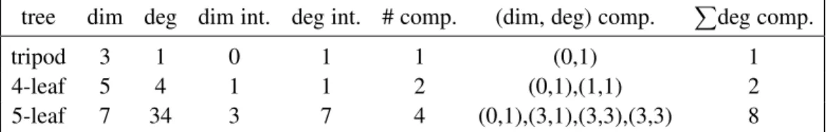
We study the maximum likelihood estimation problem for several classes of toric Fano models. We start by exploring the maximum likelihood degree for all 2-dimensional Gorenstein toric Fano varieties. We show that the ML degree is equal to the degree of the surface in every case except for the quintic del Pezzo surface with two ordinary double points and provide explicit expressions that allow one to compute the maximum likelihood estimate in closed form whenever the ML degree is less than 5. We then explore the reasons for the ML degree drop using A-discriminants and intersection theory. Finally, we show that toric Fano varieties associated to 3-valent phylogenetic trees have ML degree one and provide a formula for the maximum likelihood estimate. We prove it as a corollary to a more general result about the multiplicativity of ML degrees of codimension zero toric fiber products, and it also follows from a connection to a recent result about staged trees.
1. Introduction
Maximum likelihood estimation (MLE) is a standard approach to parameter estimation, and a fundamental computational task in statistics. Given observed data and a model of interest, the maximum likelihood estimate is the set of parameters that is most likely to have produced the data. Algebraic techniques have been developed for the computation of maximum likelihood estimates for algebraic statistical models[1; 2;24;26;27].
Themaximum likelihood degree(ML degree) of an algebraic statistical model is the number of complex critical points of the likelihood function over the Zariski closure of the model [9]. It measures the complexity of the maximum likelihood estimation problem on a model. In[27], an algebraic algorithm is presented for computing all critical points of the likelihood function, with the aim of identifying the local maxima in the probability simplex. In the same article, an explicit formula for the ML degree of a projective variety which is a generic complete intersection is derived and this formula serves as an upper bound for the ML degree of special complete intersections. Moreover, a geometric characterization of the ML degree of a smooth variety in the case when the divisor corresponding to the rational function is a normal crossings divisor is given in[9]. In the same paper an explicit combinatorial formula for the ML degree of a toric variety is derived by relaxing the restrictive smoothness assumption and allowing some mild singularities. For an introduction to the geometry behind the MLE for algebraic statistical models for discrete data the interested reader is referred to[29], which includes most of the current results on the MLE problem from the perspective of algebraic geometry as well as statistical motivation.
MSC2020: primary 62F10; secondary 13P25, 14M25, 14Q15 .
Keywords: algebraic statistics, maximum likelihood estimation, maximum likelihood degree, Fano varieties, toric varieties, toric fiber product.
This article is concerned with the problem of MLE on toric Fano varieties. Toric varieties correspond to log-linear models in statistics. Since the seminal papers by L. A. Goodman in the 1970s[21;22], log-linear models have been widely used in statistics and areas like natural language processing when analyzing cross-classified data in multidimensional contingency tables [6]. The ML degree of a toric variety is bounded above by its degree. Toric Fano varieties provide several interesting classes of toric varieties for investigating the ML degree drop. We focus on studying the maximum likelihood estimation for 2-dimensional Gorenstein toric Fano varieties, the Veronese(2,2)with different scalings and toric Fano varieties associated to 3-valent phylogenetic trees.
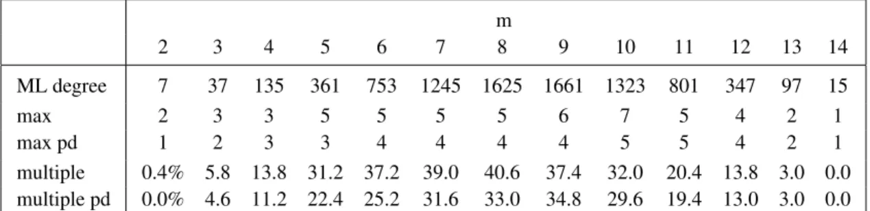
Two-dimensional Gorenstein toric Fano varieties correspond to reflexive polygons and by the classifica-tion results there are exactly 16 isomorphism classes of such polygons, see for example[33]. Out of these 16 isomorphism classes five correspond to smooth del Pezzo surfaces and 11 correspond to del Pezzo surfaces with singularities. Our first main resultTheorem 3.1states that the ML degree is equal to the degree of the surface in all cases except for the quintic del Pezzo surface with two ordinary double points. Furthermore, inTable 2, we provide explicit expressions that allow the maximum likelihood estimate to be computed in closed form whenever the ML degree is less than five.
We also explore reasons and bounds for the ML degree drop of a toric variety building on the work of Améndola et al[3]. The critical points of the likelihood function on a toric variety lie in the intersection of the toric variety with a linear space of complementary dimension. By Bézout’s theorem, the sum of degrees of irreducible components of this intersection is bounded above by the degree of the toric variety, and hence the ML degree of a toric variety is bounded by its degree. However, not all the points in the intersection contribute towards the ML degree, i.e. the points with a zero coordinate or the sum of coordinates equal to zero are not counted towards the ML degree. In the case of the quintic del Pezzo surface with two ordinary double points, the ML degree drops by two because there are two points in the intersection of the toric variety and the linear space whose coordinates sum to zero, seeExample 4.4.
These two points do not depend on the observed data byLemma 4.6. Although we do not see this
phenomenon with two-dimensional Gorenstein toric Fano varieties, the ML degree of a toric variety can drop also because the toric variety and the hyperplane intersect nontransversally, and we will see in Sections4and5that this is often the case.
Buczy´nska and Wi´sniewski proved that certain varieties associated to 3-valent phylogenetic trees are toric Fano varieties[7]. In phylogenetics, these varieties correspond to the CFN model in the Fourier coordinates. These varieties are examples of codimension zero toric fiber products as defined by Sullivant in[35]. Our second main result isTheorem 5.5that states that the MLE, ML degree as well as critical points of the likelihood function behave multiplicatively in the case of codimension zero toric fiber product of toric ideals. As a corollary, we obtain that the ML degree of the Buczy´nska–Wi´sniewski phylogenetic variety associated to a 3-valent tree is one and we get a closed form for the MLE. This result holds for the CFN model only in the Fourier coordinates, as the ML degree of the actual model in the probability coordinates can be much higher. We observe that the result about the CFN model in the Fourier coordinates can be alternatively deduced from the recent work of Duarte, Marigliano and Sturmfels[13], since Buczy´nska–Wi´sniewski phylogenetic varieties give staged tree models. It follows from the work of
Huh[28]and Duarte, Marigliano and Sturmfels[13]that the ML estimator of a variety of ML degree one is given by a Horn map, i.e. an alternating product of linear forms of specific form, and such models allow a special characterization using discriminantal triples. We discuss the Horn map and the discriminantal triple for Buczy´nska–Wi´sniewski phylogenetic varieties on 3-valent trees inExample 5.16.
The outline of this paper is the following. InSection 2, we recall preliminaries on maximum likelihood estimation, log-linear models and toric Fano varieties. InSection 3, we study the maximum likelihood estimation for two-dimensional Gorenstein toric Fano varieties. InSection 4, we explore the ML degree drop using A-discriminants and the intersection theory. Finally,Section 5is dedicated to phylogenetic models and codimension zero toric fiber products.
2. Preliminaries
2.1. Maximum likelihood estimation. Consider the complex projective spacePn−1 with coordinates
(p1, . . . ,pn). LetX be a discrete random variable taking values on the state space[n]. The coordinate pi represents the probability of thei-th eventpi=P(X=i)wherei=1, . . . ,n. Therefore p1+. . .+pn=1. The set of points inPn−1with positive real coordinates is identified with the probability simplex
1n−1= {(p1, . . . ,pn)∈Rn:p1, . . . ,pn≥0 and p1+. . .+pn=1}.
An algebraic statistical model M is the intersection of a Zariski closed subset V ⊆Pn−1 with the
probability simplex1n−1. The data is given by a nonnegative integer vector(u1, . . . ,un)∈Nn, whereui is the number of times thei-th event is observed.
The maximum likelihood estimation problem aims to find a model point p∈Mwhich maximizes the
likelihood of observing the datau. This amounts to maximizing the corresponding likelihood function
Lu(p1, . . . ,pn)=
pu1
1 · · ·p un n
(p1+. . .+pn)(u1+...+un)
over the modelM. Statistical computations are usually implemented in the affinen-planep1+. . .+pn=1. However, including the denominator makes the likelihood function a well-defined rational function on the projective spacePn−1, enabling one to use projective algebraic geometry to study its restriction to the varietyV.
he likelihood function might not be concave; it can have many local maxima, making the problem of finding or certifying a global maximum difficult. In algebraic statistics, one tries to find all critical points of the likelihood function, with the aim of identifying all local maxima[9;26;27]. This corresponds to solving a system of polynomial equations called likelihood equations. These equations characterize the critical points of the likelihood function Lu. We recall that the number of complex solutions to the likelihood equations, which equals the number of complex critical points of the likelihood function Lu over the varietyV, is called the maximum likelihood degree (ML degree) of the varietyV.
2.2. Log-linear models. In this article we are studying maximum likelihood estimation of log-linear models. From the algebraic perspective, a log-linear model is a toric variety intersected with a probability
simplex, hence linear models are sometimes called toric models. The likelihood function over a log-linear model is concave, although it can have more than one complex critical point over the corresponding toric variety intersected with the plane p1+. . .+pn=1 (there is exactly one critical point in the positive orthant). This means that in practice, algorithms like iterative proportional fitting (IPF) are used to find the MLE over a log-linear model. The closed form of the solution is in general not rational and to find its algebraic degree one needs to compute the ML degree. It is an open problem whether there is a connection
between the convergence rate of IPF and the ML degree of a log-linear model[12, Section 7.3]. The
study of the ML degree paired with homotopy continuation methods may speed up the MLE computation with respect to IPF in certain instances, as explored in[3, Section 8].
Definition 2.1. Let A=(ai j)∈Z(d−1)×n be an integer matrix. The log-linear model associated to Ais MA= {p∈1n−1:logp∈rowspan(A)}.
Alternatively, a log-linear model can be defined as the intersection of a toric variety and the probability simplex. Recall thatθaj :=θa1,j
1 θ a2,j
2 · · ·θ ad−1,j
d for j=1, . . . ,n.
Definition 2.2. Let A=(ai j)∈Z(d−1)×n be an integer matrix. The toric varietyVA⊆Rn is the Zariski closure of the image of the parametrization map
ψ:(C∗)d→(C∗)n, (s, θ1, . . . , θd−1)7→ sθa1, . . . ,sθan
.
The ideal ofVA is denoted by IAand called the toric ideal associated to A.
Often the columns of Aare lattice points of a lattice polytopeQ⊆Rd−1. In this case we say thatVAis the toric variety corresponding to Q. The log-linear modelMAis the intersection of the toric variety VA with the probability simplex1n−1. We omit Afrom the notation whenever it is clear from the context.
We conclude this subsection with a characterization of the MLE for log-linear models.
Proposition 2.3(Corollary 7.3.9 in[36]). Let A be a (d−1)×n nonnegative integer matrix and let u∈Nn be a data vector of size u+=u1+ · · · +un. The maximum likelihood estimate over the modelMA
for the data u is the unique solution pˆ,if it exists,to ˆ
p1+. . .+ ˆpn=1, Apˆ= 1
u+Au and pˆ∈MA.
Proposition 2.3is also known as Birch’s Theorem. Often we considerVAas a projective variety inPn−1. The projective version ofProposition 2.3is given inSection 4. We usually use the affine version when we want to compute the ML degree or find critical points of the likelihood function and the projective version when studying the ML degree drop.
2.3. Toric Fano varieties. In this section we will provide a brief introduction to toric Fano varieties, the main objects of study in this article. Fano varieties are a class of varieties with a special positive divisor class giving an embedding of each variety into projective space. They were introduced by Giro Fano[16] and have been extensively studied in birational geometry in the context of the minimal model program (see[31],[30]).
Definition 2.4. A complex projective algebraic variety X with ample anticanonical divisor class−KX is called aFano variety.
Two-dimensional Fano varieties are also known asdel Pezzo surfacesnamed after the Italian mathe-matician Pasquale del Pezzo, who encountered this class of varieties when studying surfaces of degreed
embedded in Pd. Throughout this paper we will use the terminology del Pezzo surface to refer to a two-dimensional Fano variety. We note that we do not use the terminology Fano surface, as a Fano surface usually refers to a surface of general type whose points index the lines on a nonsingular cubic threefold, which is not a Fano variety[15].
We will consider Fano varieties that are also toric varieties as defined inDefinition 2.2. We first focus on the characterization of two-dimensional Gorenstein toric Fano varieties, i.e. normal toric Fano varieties whose anticanonical divisorKX is not only an ample divisor but also a Cartier divisor. Isomorphism classes of Gorenstein toric Fano varieties are in bijection with isomorphism classes of reflexive polytopes, which were introduced in[5].
Definition 2.5. A lattice polytope is reflexive if it contains the origin in its interior and its dual polytope is also a lattice polytope.
In particular, toric del Pezzo surfaces are in bijection with two-dimensional reflexive polytopes. The classification of two-dimensional reflexive polytopes can be found for example in[33].
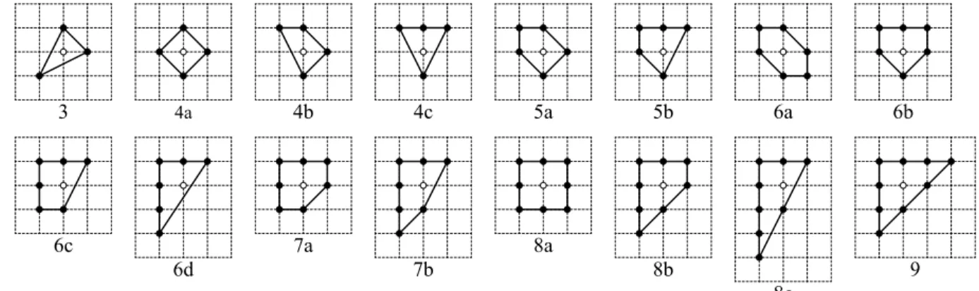
Proposition 2.6(Section 4 in[33]). There are exactly16isomorphism classes of two-dimensional reflexive polytopes,those depicted inFigure 1.
InFigure 1, the reflexive polytopes are labeled by the number of lattice points on the boundary. On the other hand, the self-intersection number K2S of the canonical class of a del Pezzo surface is thedegreeof the del Pezzo surface, which we denote byd. Here we adopt the approach of[10, Chapter 8.3], where the reflexive polytope is the one corresponding to the anticanonical embedding of the del Pezzo surface. According to[10, Chapter 8.3, Ex. 8.3.8], for each of the 16 reflexive polytopes we obtain exactly the corresponding toric del Pezzo surface. Furthermore, in[11, Chapter 8]the degree of each of these surfaces is given and coincides with the number of lattice points on the boundary. In this way, the projective
3
6c
4a 4b 4c 5a 5b 6a 6b
6d
7a
7b
8a
8b
8c
9
varieties corresponding to the polytopes labeled by 6a,7a,8a,8b and 9 are smooth and the projective varieties corresponding to the rest of the polytopes inFigure 1have singularities. The dual of the polytope labeled by numberx and letter y is in the isomorphism class of the polytope labeled by number 12−x
and letter y. This is related to the so-called “12 theorem” for reflexive polytopes of dimension 2[20]. Remark 2.7. As explained above, in the manner that toric varieties were defined inDefinition 2.2, the degree of the toric variety corresponding to a polytope Qand the number of lattice points on the boundary of Q coincide. However, sometimes in the literature (see for instance [8, Example, p. 123]) the dual polytope is used to characterize the isomorphism class of a toric del Pezzo surface. In our setting, the corresponding polytope forP2is the polytope 9 inFigure 1which gives the anticanonical embedding, i.e. the degree 3 Veronese embedding intoP9using the linear system of cubics.
3. MLE of two-dimensional Gorenstein toric Fanos
In this section we determine the ML degree of two-dimensional Gorenstein toric Fano varieties. When the ML degree is less than or equal to three, we reduce the likelihood equations to relatively simple expressions that can be used to compute a closed form for the maximum likelihood estimates. We use the cubic del Pezzo surface as an example to illustrate the MLE derivation. To avoid statistical difficulties, in all of this section we have translated reflexive polygons by a positive vector such that the resulting polygons lie minimally in the positive orthant.
Theorem 3.1. Let Sd be a two-dimensional Gorenstein toric Fano variety. InTable 1we determine the
ML degree of Sdand show that it is equal to the degree d of the surface in all cases except for the quintic
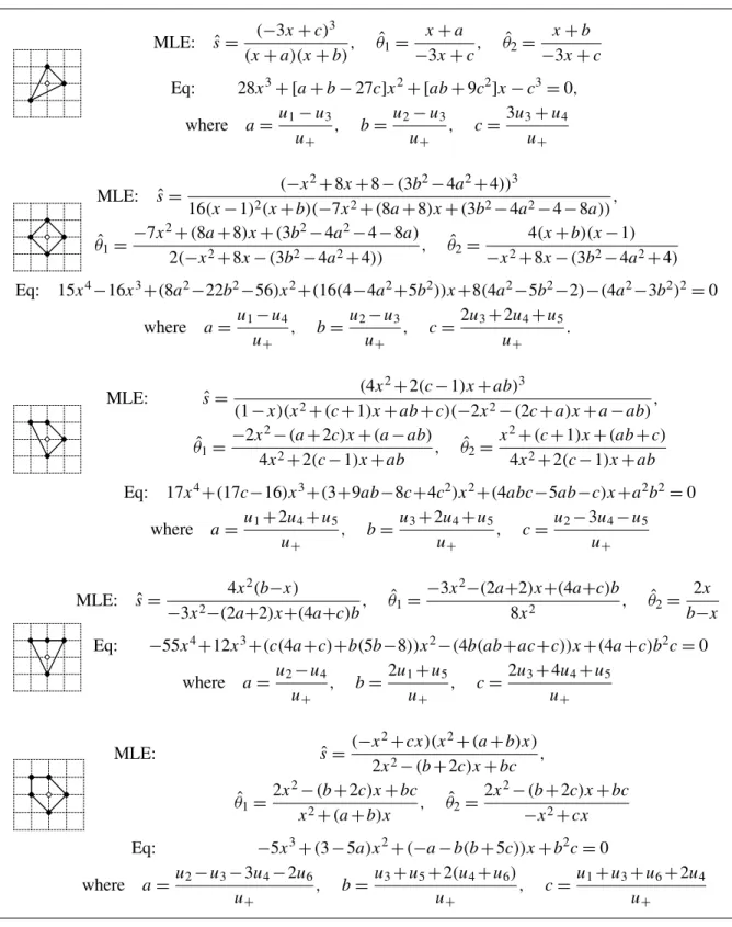
surface S5a.Table 2provides explicit expressions for computing the maximum likelihood estimate of the algebraic statistical models corresponding to the cubic S3,the quartics S4a,S4b,S4cand the quintic S5a toric two-dimensional Fano variety.
Table 1is constructed usingProposition 2.3andMacaulay2[23]. The results described inTable 1are in accordance with[29, Theorem 3.2], which states that the ML degree of a projective toric variety is bounded above by its degree. We see inTable 1that the ML degree drops to three in the case of a quintic del Pezzo surfaceS5a corresponding to the reflexive polytope 5a inFigure 1. The next section provides
an explanation of the ML degree drop in the case of the quinticS5a using the notion of A-discriminant.
Example 3.2(singular cubic del Pezzo surface). Consider the reflexive polytope
The corresponding projective toric variety is a cubic surfaceS3inP3with three singular points. Its ideal is generated by IS3= hp
3
Ideal of degree-d del PezzoSd mldeg
S3:p1p2p3−p34 3
S4a:p2p4−p1p5,p23−p1p5 4
S4b:p2p4−p23,p2p3−p1p5 4
S4c: p2p4−p32,p22−p1p5 4
S5a: p3p5−p4p6,p2p5−p26,p2p4−p3p6,p1p4−p26,p1p3−p2p6 3
S5b: p3p5−p4p6,p2p5−p26,p2p4−p3p6,p1p4−p2p6,p22−p1p3 5
S6a: p4p6−p5p7,p3p6−p27,p2p6−p1p7,p3p5−p4p7,p2p5−p27
p1p5−p6p7,p2p4−p3p7,p1p4−p27,p1p3−p2p7 6
S6b:p5p6−p1p7,p4p6−p2p7,p3p5−p4p7,p2p5−p72,p2p4−p3p7
p1p4−p27,p1p3−p2p7,p22−p3p6,p1p2−p6p7 6
S6c:p26−p5p7,p4p6−p3p7,p3p6−p2p7,p4p5−p2p7,p3p5−p2p6
p2p4−p1p7,p32−p1p7,p2p3−p1p6,p22−p1p5 6
S6d: p62−p5p7,p5p6−p4p7,p3p6−p2p7,p25−p4p6,p3p5−p2p6
p3p4−p2p5,p32−p1p6,p2p3−p1p5,p22−p1p4 6
S7a: p5p7−p4p8,p4p7−p3p8,p2p7−p1p8,p5p6−p3p8,p4p6−p3p7
p2p6−p1p7,p4p5−p2p8,p3p5−p1p8,p42−p1p8,p3p4−p1p7
p2p4−p1p5,p32−p1p6,p27−p6p8,p2p3−p1p4 7
S7b: p72−p6p8,p6p7−p5p8,p4p7−p3p8,p3p7−p2p8,p26−p5p7
p4p6−p2p8,p3p6−p2p7,p4p5−p2p7,p3p5−p2p6,p3p4−p1p8
p2p4−p1p7,p32−p1p7,p2p3−p1p6,p22−p1p5 7
S8a:p28−p7p9,p6p8−p5p9,p5p8−p4p9,p3p8−p2p9,p2p8−p1p9
p6p7−p−4p9,p5p7−p4p8,p3p7−p1p9,p2p7−p1p8,p62−p3p9
p5p6−p2p9,p4p6−p1p9,p52−p1p9,p4p5−p1p8,p3p5−p2p6
p2p5−p1p6,p42−p1p7,p3p4−p1p6,p2p4−p1p5,p22−p1p3 8
S8b:p28−p7p9,p7p8−p6p9,p5p8−p4p9,p4p8−p3p9,p2p8−p1p9
p27−p6p8,p5p7−p3p9,p4p7−p3p8,p2p7−p1p8,p5p6−p3p8
p4p6−p3p7,p2p6−p1p7,p52−p2p9,p4p5−p1p9,p3p5−p1p8
p42−p1p8,p3p4−p1p7,p2p4−p1p5,p23−p1p6,p2p3−p1p4 8
S8c:p28−p7p9,p7p8−p6p9,p6p8−p5p9,p4p8−p3p9,p3p8−p2p9
p72−p5p9,p6p7−p5p8,p4p7−p2p9,p3p7−p2p8,p26−p5p7
p4p6−p2p8,p3p6−p2p7,p4p5−p2p7,p3p5−p2p6,p42−p1p9
p3p4−p1p8,p2p4−p1p7,p23−p1p7,p2p3−p1p6,p22−p1p5 8
S9:p29−p8p10,p8p9−p7p10,p6p9−p5p10,p5p9−p4p10,p3p9−p2p10
p2
8−p7p9,p6p8−p4p10,p5p8−p4p9,p3p8−p2p9,p6p7−p4p9
p5p7−p4p8,p3p7−p2p8,p62−p3p10,p5p6−p2p10,p4p6−p2p9
p3p6−p1p10,p2p6−p1p9,p52−p2p9,p4p5−p2p8,p3p5−p1p9
p2p5−p1p8,p24−p2p7,p3p4−p1p8,p2p4−p1p7,p23−p1p6
p2p3−p1p5,p22−p1p4 9 Table 1. ML degrees of 2-dimensional Gorenstein toric Fanos.
MLE: sˆ= (−3x+c) 3 (x+a)(x+b),
ˆ θ1=
x+a −3x+c,
ˆ θ2=
x+b −3x+c
Eq: 28x3+ [a+b−27c]x2+ [ab+9c2]x−c3=0, where a=u1−u3
u+ , b=
u2−u3 u+ , c=
3u3+u4 u+
MLE: sˆ= (−x
2+8x+8−(3b2−4a2+4))3
16(x−1)2(x+b)(−7x2+(8a+8)x+(3b2−4a2−4−8a)), ˆ
θ1=
−7x2+(8a+8)x+(3b2−4a2−4−8a)
2(−x2+8x−(3b2−4a2+4)) , θˆ2=
4(x+b)(x−1)
−x2+8x−(3b2−4a2+4)
Eq: 15x4−16x3+(8a2−22b2−56)x2+(16(4−4a2+5b2))x+8(4a2−5b2−2)−(4a2−3b2)2=0 where a=u1−u4
u+ , b=
u2−u3 u+ , c=
2u3+2u4+u5
u+ .
MLE: sˆ= (4x
2+2(c−1)x+ab)3
(1−x)(x2+(c+1)x+ab+c)(−2x2−(2c+a)x+a−ab), ˆ
θ1=
−2x2−(a+2c)x+(a−ab)
4x2+2(c−1)x+ab , ˆ θ2=
x2+(c+1)x+(ab+c)
4x2+2(c−1)x+ab
Eq: 17x4+(17c−16)x3+(3+9ab−8c+4c2)x2+(4abc−5ab−c)x+a2b2=0 where a=u1+2u4+u5
u+ , b=
u3+2u4+u5
u+ , c=
u2−3u4−u5 u+
MLE: sˆ= 4x
2(b−x)
−3x2−(2a+2)x+(4a+c)b, ˆ θ1=
−3x2−(2a+2)x+(4a+c)b
8x2 ,
ˆ θ2=
2x b−x
Eq: −55x4+12x3+(c(4a+c)+b(5b−8))x2−(4b(ab+ac+c))x+(4a+c)b2c=0 where a=u2−u4
u+ , b=
2u1+u5
u+ , c=
2u3+4u4+u5 u+
5a
MLE: sˆ=(−x
2+cx)(x2+(a+b)x)
2x2−(b+2c)x+bc , ˆ
θ1=
2x2−(b+2c)x+bc x2+(a+b)x ,
ˆ θ2=
2x2−(b+2c)x+bc −x2+cx
Eq: −5x3+(3−5a)x2+(−a−b(b+5c))x+b2c=0 where a=u2−u3−3u4−2u6
u+ , b=
u3+u5+2(u4+u6)
u+ , c=
u1+u3+u6+2u4 u+
Table 2. Explicit forms for the MLE for 2-dimensional Gorenstein toric Fanos, with corresponding polytopesQd. “Eq” stands for the polynomial equation of degreed=mldeg.
We are interested in the algebraic statistical model given by the matrix
A=
2 1 0 1 1 2 0 1
.
This nonnegative integer matrix Agives the parametrization map
f :C3→C3,(s, θ1, θ2)7→(sθ12θ2,sθ1θ22,s,sθ1θ2).
After applying Birch’s theorem, we can write the unique maximum likelihood estimatesˆ,θˆ for the datau as(sˆ,θˆ1,θˆ2)=(pˆ34/(pˆ1pˆ2),pˆ1/pˆ4,pˆ2/pˆ4), where
ˆ
p1=x+a, pˆ2=x+b, pˆ4= −3x+c,
witha=u1−u3 u+ ,b=
u2−u3 u+ ,c=
3u3+u4
u+ andx is given by
28x3+ [(a+b)−27c]x2+ [ab+9c2]x−c3=0.
Remark 3.3. When the ML degree of the del Pezzo surface is greater than or equal to five, the maximum likelihood estimate pˆi,i=1, . . . ,nsatisfies an equation of degree five or higher. By the Abel–Ruffini theorem there is no algebraic solution for a general polynomial equation of degree five or higher, therefore one would expect that it is not possible to obtain a closed form solution for the maximum likelihood estimate in these cases. However, one can then turn to numerical algebraic geometry methods to compute the MLE (see e.g. [26]).
4. ML degree drop
In order to understand why the ML degree is lower than the degree for the quintic del Pezzo surface 5a, it is useful to think of different embeddings of a toric variety via scalings and how these affect the ML degree. For a full analysis see[3].
Let Q⊆Rd−1 be a lattice polytope withn lattice pointsaj ∈Zd−1. Define Ato be the(d−1)×n matrix with the columns a1, . . . ,an. A scaling c∈ (C∗)n can be used to define the parametrization
ψc : (
C∗)d→(C∗)n as
ψc(s, θ
1, . . . , θd−1) = (c1sθa1, . . . ,cnsθan).
We denote byVc the Zariski closure of the image of the monomial mapψc. The usual parametrization of the toric variety is whenc=(1, . . . ,1). We then denote the corresponding toric variety byV =V(1,...,1). Definition 4.1. TheML degree dropof a scaled toric varietyVc is the difference deg(V)−mldeg(Vc).
Define fc=Pin=1ciθ
ai wherec=(c
1, . . . ,cn)∈(C∗)n.
Definition 4.2. To any matrix Aas above, one can associate the variety
∇A=
c∈(C∗)n| ∃θ ∈(
C∗)d−1 such that f c(θ)=
∂fc
∂θi (θ)
=0 for alli
This is the Zariski closure of the set of scalingsc ∈(C∗)n such that the hypersurface {fc =0} has a singular point in(C∗)d−1. IfPλ
jaj:λj ∈Z,
P
λj =1 =Zd−1— that is, if the affine lattice generated by Ais the full integer lattice — then the variety∇A is a hypersurface. In this case, it is defined by an
irreducible polynomial denoted1A, called the A-discriminant[19, Chapter 8]. The main object that determines whether the ML degree drops is the polynomial:
EA(c) =
Y
0face ofQ
10∩A(c) (4-1)
where the product is taken over all nonempty faces0⊂Qincluding Q itself and0∩Ais the matrix whose columns correspond to the lattice points contained in0. Under certain conditions this is precisely theprincipal A-determinant[19, Chapter 10].
Theorem 4.3(Theorem 2 in[3]). Let Vc⊂Pn−1be the scaled toric variety defined by the monomial parametrization with scaling c∈(C∗)nfixed. Thenmldeg(Vc) <deg(V)if and only if EA(c)=0.
Example 4.4. We will explain why forc=(1,1, . . . ,1), the ML degree of the quintic del Pezzo 5b is 5 (and thus equal to its degree), while the ML degree of the quintic del Pezzo 5a is strictly less than 5.
Let us consider first the case of the quintic del Pezzo 5b (see figure on the right).
5b
We can label its lattice points and arrange them in the matrix
A=
0 0 1 1 1 2 1 2 0 1 2 2
We have to check that forc = (1, . . . ,1), EA(c)6= 0. By (4-1), the polynomial
EA(c)is a product of0∩A-discriminants. Verticesai have1ai =1. Analogously, edges of lattice length one cannot have nontrivial discriminant (the lattice length of an edge is the number of lattice points contained in the edge minus one). The only potential edgeethat may be relevant here is the one of lattice length 2. The corresponding fc,e=c02y2+c12x y2+c22x2y2 has a nontrivial singularity if and only if c02+c12x+c22x2does, thus1e(c)=c212−4c02c22. Note it is nonzero forc=(1, . . . ,1).
It only remains to check that(1, . . . ,1) /∈ ∇A. The followingM2 computation verifies that forc= (1, . . . ,1), fc=y+y2+x+x y2+x2y2+x y has no singularities:
R = QQ[x,y]
J = ideal(y+y^2+x+x*y^2+x^2*y^2+x*y, 1+y^2+2*x*y^2+y, 1+2*y+2*x*y+2*x^2*y+x)
gens gb J
The last command returns that the Gröbner basis forJ is{1}. Now, for the quintic
5a
del Pezzo 5a, we identify the matrix
A=
0 0 1 1 1 2 1 2 0 1 2 1
.
All edges are of lattice length one, so we again focus on∇A. However, nowc=(1, . . . ,1)∈ ∇A, as the following code verifies.
I = ideal(y+y^2+x+x*y^2+x^2*y+x*y, 1+y^2+2*x*y+y, 1+2*y+2*x*y+x^2+x) gens gb I
In this case we get 2 points, the solutions of x +y =0,y2−y−1 = 0, as singularities for fc =
y+y2+x+x y2+x2y+x y. The corresponding points of the variety are
(1/2(1+ √
5),1/2(3+ √
5),−1/2(1+ √
5),−1/2(3+ √
5),−2− √
5,2+ √
5),
(1/2(1− √
5),1/2(3− √
5),−1/2(1− √
5),−1/2(3− √
5),−2+ √
5,2− √
5).
(4-2)
According toTheorem 4.3, the ML degree must drop for 5a.
Remark 4.5. The singular locus of the quintic del PezzoS5a consists of the two points(0,0,1,0,0,0) and (0,0,0,0,0,1) which are both rational double points. These points are different from the two points(4-2)that cause the ML degree drop.
Theorem 4.3characterizes scaling factorscsuch that the ML degree ofVcis less than the degree ofV. All critical points of the likelihood function ofVc lie in the intersection ofV with a linear space. In the rest of this section, we will investigate the ML degree drop for a given toric varietyVcby studying this intersection.
Let Lc(p)=Pni=1cipi and Lc,i(p)= Pn
j=1Ai jcjpj fori =1, . . . ,d−1. These polynomials are
implicit versions of the polynomials fc andθi∂∂θfc i for i
=1, . . . ,d−1. By [3, Proposition 7]the ML
degree of Vc is the number of points pinV\V(p1· · ·pn(c1p1+. . .+cnpn))satisfying
(Au)iLc(p)=u+Lc,i(p) fori=1, . . . ,d−1 (4-3) for generic vectorsu. DefineL0c,u to be the intersection ofV with the solution set of(4-3)andLc,u to be the intersection of V\V(p1· · ·pn(c1p1+. . .+cnpn))with the solution set of(4-3). By[18, Example 12.3.1], the sum of degrees of the irreducible components ofL0c,u is at most degV.
The obvious reason for the ML degree drop comes from removing these irreducible components of L0
c,u that belong toV(p1· · ·pn(c1p1+. . .+cnpn)). We will see in Lemma 4.6that the irreducible components ofL0
c,u that are removed do not depend onu but only oncand the varietyV. In the case of the toric del Pezzo surface 5a, the ML degree drop is completely explained by this reason. The degree of this del Pezzo surface is five. The varietyL0c,u consists of two zero-dimensional components of degrees three and two. The degree two component consists of two points(4-2)that lie in the variety V(p1· · ·pn(c1p1+. . .+cnpn))and hence is removed.
Lemma 4.6. The points inL0
c,u\Lc,u are independent of u. They are exactly the points p∈V that satisfy
Lc(p)=Lc,1(p)=. . .=Lc,d−1(p)=0.
Proof.Any p∈V satisfyingLc(p)=Lc,1(p)=. . .=Lc,d−1(p)=0 is inL0c,u\Lc,ufor anyu. Conversely, by the proof of[3, Theorem 13], if p∈L0
c,u\Lc,u, then Lc(p)=0. It follows from equations(4-3)that
then also Lc,i(p)=0 fori=1, . . . ,d−1. But then psatisfies(4-3)for anyu.
The more complicated reason for the ML degree drop can be the nontransversal intersection of V
a1 a2 a3 a4
a5
a6
Figure 2. Polytope Qcorresponding to the smooth Fano varietyP2. transversally at p∈A∩B if pis a smooth point of A,B and
TpA+TpB=TpPn.
The intersection of A and B is generically transverse if it is transverse at a general point of every component of A∩B. If the intersection ofV and the linear subspace defined by(4-3)is not generically transverse, the sum of degrees of the irreducible components ofL0
c,u can be less than deg(V), in which case also the ML degree of the toric varietyVc is less than the degree of the toric variety V. One could think that the intersection of V and the linear subspace defined by(4-3)is generically transverse for generic vectorsu, but since the linear subspace defined by (4-3)depends on the variety V, then the intersection is not necessarily generically transverse. We will see several such examples later in this section and inSection 5. We note that the sum of degrees of the irreducible components can be less that degV even if the degrees are counted with multiplicity as in[18, Example 12.3.1].
Corollary 4.7. The ML degree dropdeg(V)−mldeg(Vc)is bounded below by the sum of degrees of the irreducible components of the intersection of V and the linear subspace defined by Lc(p)=Lc,1(p)= . . .=Lc,d−1(p)=0. If the intersection of V and the linear subspace defined by(4-3) is generically transverse,then this bound is exact.
InCorollary 4.7, we consider only irreducible components whose ideals are different fromhp1, . . . ,pni as we work over the projective space.
Proof. The sum of degrees of the irreducible components of L0
c,u is at most deg(V)by[18, Example 12.3.1]and the number of elements ofLc,u is mldeg(Vc). ByLemma 4.6, we obtainLc,u fromL0c,u by removing all the irreducible components that satisfy Lc(p)=Lc,1(p)=. . .=Lc,d−1(p)=0. Hence the
difference of the sum of degrees of the irreducible components ofL0c,u and the number of elements of Lc,uis the sum of degrees of the irreducible components of the intersection ofV and the linear subspace defined by Lc(p) = Lc,1(p)=. . . = Lc,d−1(p) =0. If V and the linear subspace defined by (4-3)
intersect generically transversely, then the sum of degrees of the irreducible components ofL0
c,u is equal
to degV.
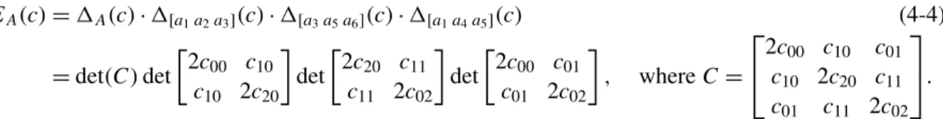
To understand the above observations, we analyze the different ML degree drops corresponding to the quadratic Veronese embedding ofP2given by the Fano polytope inFigure 2.
In[3, Example 26], it was shown that different scalingsc∈R6 produce ML degrees ranging from 1 to 4, under several combinations of the vectorclying on each of the discriminants making up the principal
A-determinant, defined by
EA(c)=1A(c)·1[a1a2a3](c)·1[a3a5a6](c)·1[a1a4a5](c)
=det(C)det
2c00 c10 c10 2c20
det
2c20 c11 c11 2c02
det
2c00 c01 c01 2c02
, whereC=
2c00 c10 c01 c10 2c20 c11 c01 c11 2c02
.
(4-4)
The different combinations are presented in[3, Table 2], which we reproduce here inTable 3(while fixing some typos). In each line, we go further than identifying a possible drop and actually explain the exact drops observed.
Naively, each appearance of a 0 in a row ofTable 3makes the ML degree drop by 1. But this cannot be, since the last row has all four zeros and the ML degree cannot drop to 0. We will see in the explanation of the last two rows that it is in general impossible to predict the exact drop just from knowing in what discriminants the vectorclies.
C 1A 1[a1a2a3] 1[a3a5a6] 1[a1a4a5] mldeg
2 1 1 1 2 1 1 1 2
6=0 6=0 6=0 6=0 4
2 2 1 2 2 3 1 3 2
6=0 0 6=0 6=0 3
2 2 1 2 2 2 1 2 2
6=0 0 0 6=0 2
-2 2 2 2 -2 2 2 2 -2
6=0 0 0 0 1
17 22 27 22 29 36 27 36 45
0 6=0 6=0 6=0 3
2 3 3 3 5 5 3 5 5
0 6=0 0 6=0 2
2 2 2 2 2 2 2 2 2
0 0 0 0 1
• Row 1This corresponds to the generic case. The intersectionL0
c,uis transverse and zero-dimensional with 4 points, corresponding to the ML degree. There are no points inL0
c,u\Lc,u and there is no drop.
• Row 2When computing the points in VA∩ {Lc(p)=Lc,1(p)=. . .=Lc,d−1(p)=0}we obtain the
unique projective point[1: −1:1:0:0:0], which makes the A-discriminant of the edge[a1,a2,a3]
of Qvanish. Removing this point gives the ML degree of 3=4−1.
• Row 3Now we have one more point in the removal set: apart from the one in the above row, there is
also[0:0:1:0:1: −1]on the zero locus of the A-discriminant of the edge[a3,a5,a6]. The drop
is accounted for exactly these two points and we have ML degree 2=4−2. • Row 4There are three points inL0
c,u\Lc,u that lie on the zero loci of edge A-discriminants: [1:1: 1:0:0:0]for the edge[a1,a2,a3],[0:0:1:0:1:1]for the edge[a3,a5,a6]and[1:0:0:1:1:0]
for the edge[a1,a4,a5]. They explain the drop in ML degree 1=4−3.
• Row 5The only removal point is[1: −2:4:1:1: −2], which doesnotlie on zero loci of any of the A-discriminants of the edges ofQ, but only on the zero locus of the A-discriminant of the whole of Q. Removing this point gives the ML degree of 3=4−1.
• Row 6This is the first time that the removal ideal IA+Lc(p),Lc,1(p), . . . ,Lc,d−1(p)
is not radical. While there is only one point,[0:0:1:0:1: −1], its multiplicity is 2. We used theMacaulay2
packageSegreClasses[25]to compute the multiplicity. The intersectionL0
c,u is zero-dimensional but consists of two components of degree 2. The first component is prime and corresponds to the two points in the ML degree 2. The toric variety and the linear space defined by (4-3)intersect transversely at both points of the first component. The second component is primary, but not prime. Its radicalhp6+p5,p4,p3+p5,p2,p1iis a zero-dimensional ideal of degree 1, corresponding to
the above point that lies on the zero locus of the A-discriminant of the edge[a3,a5,a6].
Although the intersection of the toric variety and the linear space defined by(4-3)is dimensionally transverse, it is not transverse at the point defined by the second component. We also observe that while1A(c)=0, there is no singular point of fc, which means c lies strictly in the closure in Definition 4.2(seeRemark 4.8below).
• Row 7Now the removal ideal is 1-dimensional of degree 2. It is given by
p22+p2p3+p3p4, p1+p2+p4, p2+p5−p2−p3, p2+p3+p6.
Its variety intersects V0∩A in one point for each edge0 of Q. In other words, the reason why all discriminants1[a1a2a3], 1[a3a5a6], 1[a1a4a5]vanish is that the removal set intersects the planes
p1=p2=p4=0, p2=p3=p6=0 and p4=p5=p6=0 respectively, and one can find in each
a point with complementary support. Furthermore, it intersects the open set where none of the pi are zero, which explains why1A=0 too. Unfortunately, this alone does not explain why the ML degree is 1.
By looking at the intersection ideal of the toric varietyVA with the equations(4-3), we realize that the intersection is not transverse (not even dimensionally transverse). Indeed, there are two
components: a zero-dimensional component of degree 1 (corresponding to the MLE) and a one-dimensional component of degree 2 (so the sum of the degrees is 1+2=3<4). This last component matches the removal ideal above. At the 0-dimensional component the toric variety intersects the linear space defined by(4-3)transversely. At a generic point of the 1-dimensional component the intersection is not transverse. Both components have multiplicity one and hence also the sum of degrees counted with multiplicity is less than four.
Remark 4.8. If for some scalingc, theA-discriminant of at least one edge is zero and theA-discriminant of at least one edge is nonzero, then there is no singular pointθ ∈(C∗)2 of fc. Indeed, such a point
θ =(θ1, θ2)∈(C∗)2 would need to satisfy
2c00 c10 c01 c10 2c20 c11 c01 c11 2c02
1 θ1 θ2 = 0 0 0
. (4-5)
Say 1[a3a5a6] = det
2c20 c11
c11
2c02
= 0 . In order for the system (4-5) to be consistent, c10 c01
2c20 c11
c11
2c02
should have rank 1. In particular, detc10
2c20 c01 c11
=0 and detc10 c11
c01
2c02
=0, which in turn means that both 2c00
c10 c10
2c20 c01 c11
and2c00 c01
c10 c11
c01
2c02
have rank 1. We conclude thatC itself must have rank 1, so thatcmust lie in the discriminants of all the edges (as in Row 7), contradicting that one of them was nonzero. This means that if we are in the case of Row 6, even though1A(c)=0, the scalingc∈ ∇A is added in the closure that appears inDefinition 4.2.
Conjecture 4.9. The intersection of V and the linear space given by(4-3)is generically transverse at the irreducible component ofL0
c,u that gives the MLE.
This conjecture holds for all the examples considered in this section. At other irreducible components the intersection may or may not be transverse.
Remark 4.10. For toric models,
mldeg(V)=χtop(V\H)=χtop(V)−χtop(V ∩H) (4-6)
whereH = {p|p1· · ·pn(p1+ · · · +pn)=0}andχtop is the topological Euler characteristic. The first
equality was proved by Huh and Sturmfels[29, Theorem 3.2], and the second equality is the excision formula. The Euler characteristic of toric del Pezzo surfaces can be computed byχtop(V)=2+rkPic(V).
The rank of the Picard group rkPic(V)can be computed taking into account that the minimal resolution of every del Pezzo surface is a product of two projective linesP1×P1 (polytope 8a inFigure 1), the
quadric cone P(1,1,2)⊂P3(polytope 8c inFigure 1), or the blow-up of a projective plane in 9−d
points in almost general position; namely at most three of which are collinear, at most six of which lie on a conic, and at most eight of them on a cubic having a node at one of the points. We refer the reader to [11]for a more detailed study of this classical subject of algebraic geometry. It would be interesting to explore the ML degree drop further from this perspective.
5. Toric fiber products and phylogenetic models
In [7], Buczy´nska–Wi´sniewski study an infinite family of toric Fano varieties that correspond to 3-valent phylogenetic trees. These Fano varieties are of index 4 with Gorenstein terminal singularities. In phylogenetics, these varieties correspond to the CFN model in the Fourier coordinates. We define them through the corresponding polytopes.
Definition 5.1. LetT be a 3-valent tree, i.e. every vertex ofT has degree 1 or 3. Consider all labelings of the edges ofT with 0’s and 1’s such that at every inner vertex the sum of labels on the incident edges is even. Define PT ⊆RE to be the convex hull of such labelings. LetIT be the homogeneous ideal and
VT be the projective toric variety corresponding to PT.
Example 5.2. If T is tripod, then PT =conv((0,0,0), (1,1,0), (1,0,1), (0,1,1)) is a simplex and
VT =P3is the 3-dimensional projective space.
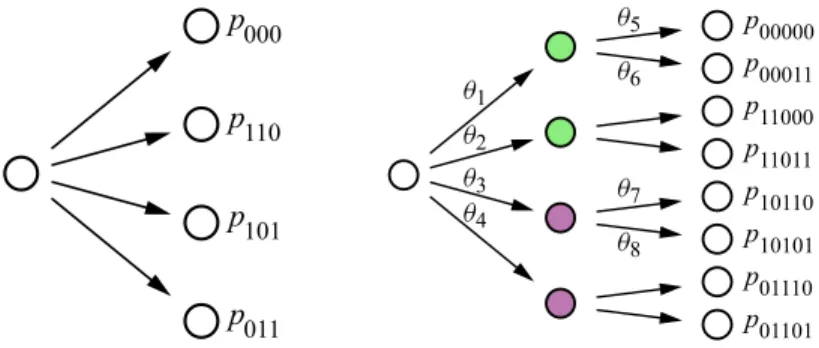
Example 5.3. IfT is the unique 3-valent four leaf tree, then
PT =conv((0,0,0,0,0), (1,1,0,0,0), (0,0,0,1,1), (1,1,0,1,1),
(1,0,1,1,0), (1,0,1,0,1), (0,1,1,1,0), (0,1,1,0,1)).
The idealIT is generated by the two quadratic polynomialsx00000x11011−x11000x00011andx10110x01101− x01110x10101.
The aim of the rest of the section is to show that if T is a 3-valent tree then the ML degree of the varietyVT is one. We will also give a closed form for its maximum likelihood estimate. This result will be a special case of a more general result about ML degrees of codimension-0 toric fiber products of toric ideals. A toric fiber product can be defined for any two ideals that are homogenous by the same multigrading [35], however, we use the definition specific to toric ideals [14, Section 2.3]. Besides phylogenetic models considered in this section, codimension-0 toric fiber products appear in general group-based models in the Fourier coordinates and reducible hierarchical models (see[35, Section 3]for details on applications).
Letr∈Nandsi,ti ∈Nfor 1≤i≤r. We consider toric ideals corresponding to vector configurations B= {bij :i∈ [r], j∈ [si]} ⊆Zd1 andC= {cki :i∈ [r],k∈ [ti]} ⊆Zd2. These toric ideals are denoted by
IBand IC, they live in the polynomial ringsR[xij :i∈ [r], j∈ [si]]andR[y i
k:i∈ [r],k∈ [ti]], and they are required to be homogeneous with respect to the multigrading byA= {ai:i∈ [r]} ⊆Zd. We assume
that there existsω∈Qd such thatωai =1 for alli, so thatIBand IC are homogeneous also with respect to the standard grading. Toric ideals IB and IC being homogeneous with respect to the multigrading byAimplies that there exist linear mapsπ1:Zd1 →Zd andπ2:Zd2 →Zd such thatπ1(bij)=a
i and
π2(cik)=a
i. We define the vector configuration
B×AC= {(bij,cki):i∈ [r], j∈ [si],k∈ [ti]}.
The toric fiber product ofIBand IC with respect to the multigrading byAis defined as
and it lives in the polynomial ringR[zij k:i∈ [r], j∈ [si],k∈ [ti]].
Example 5.4. LetT be a 3-valent tree withn≥4 leaves. WriteT as a union of two treesT1and T2
that share an interior edge e. Taker =2. Let b1j be the vertices of PT1 that have label 0 on edgee and letb2j be the vertices of PT1 that have label 1 on edgee. Define similarlyck1and c2k for PT2. Let A= {(0,1), (1,0)}, so thatπ1 mapsb1j to(0,1)andb2j to(1,0). ThenIT is the toric fiber product of
IT1 and IT2 with respect to multigrading byA. In[35, Section 3.4]the toric fiber product construction is explained in full generality for group-based phylogenetic models in the Fourier coordinates.
Given a vectoru indexed by the elements of B×AC, we denote its entries byuij k for i∈ [r], j∈ [si],k∈ [ti]. We defineui++=
P
j∈[si],k∈[ti]u i
j k,u i
j+= P
k∈[ti]u i
j k andu i
+k =
P
j∈[si]u i
j k. We denote the corresponding vectors byuA,uBanduC since they are indexed by the elements ofA,BandC. These vectorsuA=(ui++)i∈[r],uB=(uij+)i∈[r],j∈[si]anduC=(u
i
+k)i∈[r],k∈[ti]are marginal sums. We also define
u+++= P
i∈[r],j∈[si],k∈[ti]u i
j k,(uB)
+ +=
P
i∈[r] P
j∈[si](u i
j+)and(uC)
+ +=
P
i∈[r] P
k∈[ti](u i
+k). Similarly, if pij kis a joint probability distribution indexed by the elements ofB×AC, the sum of the joint probability distribution overA(resp.B,C) is a marginal probability distribution and we denote it by pA=(pi++)i∈[r]
(resp. pB=(pij+)i∈[r],j∈[si], pC =(p i
+k)i∈[r],k∈[ti]).
Theorem 5.5. LetAconsist of linearly independent vectors. Then the ML degree of IB×AIC is equal
to the product of the ML degrees of IBand IC. For a data vector u,every critical point of the likelihood
function has the form
pij k:= (pB)
i j(pC)
i k
(pA)i ,
(5-1)
where pA, pBand pC are critical points of the likelihood function for the models IA, IBand IC and data
vectors uA,uBand uC,respectively. Since the elements ofAare linearly independent, pAis in fact the
normalized uA. Moreover,we obtain the maximum likelihood estimate of IB×AIC by taking pA, pBand
pC to be the maximum likelihood estimates of the models IA, IBand IC.
Theorem 5.5generalizes known results about reducible hierarchical[34, Proposition 4.14]and discrete graphical models. In particular, one recovers the rational formula for the MLE in the case of decomposable graphical models (indeed, they have ML degree one)[34, Proposition 4.18]and general discrete graphical models[17, Theorem 1]. The latter result is for mixed graphical interaction models that allow both discrete and continuous random variables.Theorem 5.5generalizes the case when all variables are discrete.
To proveTheorem 5.5, we first have to recall how to obtain a generating set for IB×AIC from the generating sets for IB andIC. Let
f =xi1 j1 1
xi2 j1 2
· · ·xid j1 d
−xi1 j2 1
xi2 j2 2
· · ·xid j2 d
∈R[xij].
Fork=(k1,k2, . . . ,kd)∈ [ti1] × [ti2] × · · · × [tid]define
fk=zij11 1k1
zi2 j21k2
· · ·zid jd1kd
−zi1 j12k1
zi2 j22k2
· · ·zid jd2kd
LetTf =Qdl=1[til]. For a set of binomialsF, we define
Lift(F)= {fk : f ∈F,k∈Tf}. We also define
Quad= {zij
1k1z i
j2k2−z i j1k2z
i
j2k1:i∈ [r],j1, j2∈ [si],k1,k2∈ [ti]}.
Proposition 5.6([35], Corollary 14). LetAconsist of linearly independent vectors. Let F be a generating set of IBand let G be a generating set of IC. Then IB×AIC is generated by
Lift(F)∪Lift(G)∪Quad.
Example 5.7. The 3-valent four leaf treeT4is the union of two tripodsT3that share an interior edgee. By
Proposition 5.6, a generating set forIT4 is given by the lifts of generating sets forIT3 and by quadrics with respect to the edgee. Since IT3 = h0i, its lift is{0}. The set Quad consists ofx00000x11011−x11000x00011
andx10110x01101−x10101x01110that are generators of IT4.
Example 5.8. The 3-valent five leaf treeT5is the union of the 3-valent four leaf treeT4and tripodT3that
share an interior edgee. The fifth index of a variablexe1e2e3e4e5 in the coordinate ring ofT4 and the first index of a variablexe5e6e7 in the coordinate ring ofT3correspond to the edgee. Recall that a generating set ofIT4 isF= {x00000x11011−x11000x00011,x10110x01101−x01110x10101}and a generating set ofIT3 isG= {0}. Both elements of F have four lifts corresponding tok=(000,110),k=(000,101),k=(011,110)and k=(011,101). Hence Lift(F)consists of
x0000000x1101110−x1100000x0001110,x0000000x1101101−x1100000x0001101, x0000011x1101110−x1100011x0001110,x0000011x1101101−x1100011x0001101, x1011000x0110110−x0111000x1010110,x1011000x0110101−x0111000x1010101, x1011011x0110110−x0111011x1010110,x1011011x0110101−x0111011x1010101,
and Lift(G)= {0}. The set Quad consists of 12 polynomials.
To proveTheorem 5.5, we also need the following lemmas.
Lemma 5.9. For any u∈RB×AC,we have(B×AC)u=(BuB,CuC).
Proof.Assume that ther-th row comes from theBpart of the matrixB×AC. Then ther-th row ofB×AC multiplied withugives
X
i∈[r],j∈[si],k∈[ti]
(bij,cki)ruij k=
X
i∈[r],j∈[si],k∈[ti]
(bij)ruij k=
X
i∈[r],j∈[si]
(bij)ruij+.
This is ther-th row ofBmultiplied withuB.
Lemma 5.10. The following equations hold:
pB=pB and pC =pC.
In particular,the entries of p sum to one i.e. p+++= P
i∈[r] P
j∈[si]
P
k∈[ti]p i
Proof. By the definition of p, we have
(pB)ij = X
k∈[ti]
(pB)ij(pC) i k
(pA)i
=(
pB)ij(pC) i
+ (pA)i
.
Hence we need to show that (pC)i+=(pA)i. By Birch’s theorem for IC, we haveCpC =C(uuC C)++ and henceπ2(C)pC =π2(C)(uuC
C)++ whereπ2is applied to
C columnwise. The second equation is equivalent
toP
i∈[r]tia
i(p C)i+=
P
i∈[r]tia
i(uC)i+
(uC)++. Since
ai are linearly independent, this implies(pC)i+= (uC)i+
(uC)++
=
ui ++ u+++
=(pA)i for alli∈ [r].
Proof ofTheorem 5.5.We start by showing that every vector of the form(5-1)satisfies the conditions of Birch’s theorem, i.e. p+++=1,(B×AC)p=(B×AC)uu+
++ and
p∈V(IB×AIC), and hence is a critical point of the likelihood function of IB×AIC. The entries of psum to one byLemma 5.10. Secondly, we have
(B×AC)p=(BpB,CpC)=(BpB,CpC)=(B
uB
(uB)++ ,C uC
(uC)++
)=(B uB
u+++ ,C uC
u+++
)=(B×AC) u
u+++ .
The first and last equalities hold byLemma 5.9. The second equality holds byLemma 5.10while the
third equality follows from Birch’s theorem for IBand IC. Thirdly, we have to showu∈IB×AIC. For
fk∈Lift(F), we have
fk(p)=
(pB)ij11 1(
pC)ik11
(pA)i1
(pB)ij21 2(
pC)ik22
(pA)i2
· · · (pB)ijd1
d(
pC)ikdd
(pA)id
− (pB)ij12
1(
pC)ik11
(pA)i1
(pB)ij22 2(
pC)ik22
(pA)i2
· · · (pB)ijd2
d(
pC)ikdd
(pA)id
=
(pB)ij11 1(
pB)ij21 2
· · ·(pB)ijd1 d
−(pB)ij12 1(
pB)ij22 2
· · ·(pB)ijd2 d
(pC)ik1
1
(pA)i1
(pC)ik22
(pA)i2
· · ·(pC)
id kd
(pA)id
= f(pB)·
(pC)ik11
(pA)i1
(pC)ik22
(pA)i2
· · ·(pC)
id kd
(pA)id
=0.
An element of Quad gives
(zij
1k1z i
j2k2−z i
j1k2z i
j2k1)(p)=
(pB)ij1(pC) i k1
(pA)i
(pB)ij2(pC) i k2
(pA)i
−(pB)
i j1(pC)
i k2
(pA)i
(pB)ij2(pC) i k1
(pA)i
=0.
Hence p is a critical point of the likelihood function ofIB×AIC.
Conversely, let pbe any critical point of the likelihood function ofIB×AIC. Then the entries of pB and pC sum to one. Also
(B uB
(uB)++ ,C uC
(uC)++
)=(B uB
u+++ ,C uC
u+++
)=(B×AC) u
u+++
=(B×AC)p=(BpB,CpC).
For every f in a generating set for IB
f(pB)= X
k∈Tf
whereck are integer coefficients. By Birch’s theorem, pB is a critical point of the likelihood function of IB and similarly pC is a critical point of the likelihood function of IC. It is left to show that pis the only element in IB×AIC with marginals pB and pC. Indeed, for fixedi ∈ [r], the matrix of pij k for
j∈ [si],k∈ [ti]has rank 1, because Quad contains all 2×2-minors for this matrix. Hence the marginals
pij+ and p
i
+k completely determine this matrix.
Finally, we get the maximum likelihood estimate ofIB×AIC by taking pBand pC to be the maximum likelihood estimates of the modelsIB andIC. ByLemma 5.10, the margins pˆB and pˆC of the maximum likelihood estimate of the modelIB×AICare equal to pBand pC, in particular pBand pC are nonnegative. By Proposition 2.3, for each toric model there is a unique nonnegative critical point of the likelihood function and it is the maximum likelihood estimate. Hence pBand pC have to be the maximum likelihood
estimates for the models IB andIC.
Let T be an n-leaf 3-valent tree. We denote the coordinates of a vector u ∈R2n−1 byul wherel corresponds to a labeling of the edges of T. Let T0
be a subtree of T and denote the restriction of the labelingl to T0 byl|T0. We denote by uT0 the marginal sum ofu with the edges of T not inT0 marginalized out, i.e. the vectoruT0 is indexed by the labelings ofT0 and ifl0 is a labeling ofT0 then
(uT0)l0 =P
l|T0=l0ul. If the subtree is an edgee, then the marginal sum is defined in the same way and denoted byue. As before, we denote the sum of entries ofubyu+.
Corollary 5.11. For any3-valent treeT,the ML degree of VT is one. IfT is tripod and u is a data vector,
then the maximum likelihood estimate is
ˆ p= u
u+ .
ItT has more than three leaves,letT1,T2, . . . ,Tn−2be the tripods contained inT and let e1,e2, . . . ,en−3 be the inner edges ofT. For data vector u,the maximum likelihood estimate is
ˆ pl =
Q
j=1,...,n−2(dpTj)l|Tj
Q
j=1,...,n−3(cpej)l|e j
, (5-2)
where pcej is the normalized uej,anddpTj is the maximum likelihood estimate for the treeTj and the data vector uTj.
The ML degree of a group-based phylogenetic model in probability coordinates is not known to be related to the ML degree in the Fourier coordinates. In particular, the ML degree can be much larger in the probability coordinates than the one in the Fourier coordinates [27, Section 6]. In probability coordinates, numerical methods are needed already in the smallest cases to determine the maximum likelihood estimate and the critical points of the likelihood function[32].
Example 5.12. LetT be the 3-valent four leaf tree, letT1 andT2be the tripods contained inT, and lete
be the inner edge ofT. We consider the data vector
with a total of 100 observations. Then
uT1 =(u000++,u110++,u101++,u011++)=(44,10,21,25), uT2 =(u++000,u++110,u++101,u++011)=(22,35,11,32),
ue=(u++0++,u++1++)=(54,46).
Since theVT1 =VT2 =P3, we have
c pT1 =(
44 100, 10 100, 21 100, 25
100),cpT2 =(
22 100, 35 100, 11 100, 32
100)andcpe =(
54 100,
46 100). Then by(5-2)
ˆ
p00000=(c
pT1)000(cpT2)000 (cpe)0
=44·22·100
1002·54 =
121 675.
Similarly, we can find other coordinates of the maximum likelihood estimate. This gives
ˆ p= 121 675, 11 270, 176 675, 8 135, 147 920, 231 4600, 35 184, 11 184 .
We obtain the same result when using Birch’s theorem.
Recent work on rational maximum likelihood estimators establishes that a class of tree models known as staged trees have ML degree 1[13, Proposition 12]. In light ofCorollary 5.11, it is natural to ask if there is any relation between staged tree models and 3-valent phylogenetic tree models. We find that this is the case in the proposition below. In fact, we believe that any codimension zero toric fiber product can be viewed as a generalized staged tree and this is left as a future research direction. Conversely, Ananiadi and Duarte study when staged trees are codimension-0 toric fiber products in the recent paper[4].
Consider a rooted treeT with at least two edges emanating from every non-leaf vertex ofT. Consider a labeling of the edges ofT by the elements of a setS. Thefloretassociated with a vertexvis the multiset of labels of edges emanating fromv. The treeT is called astaged treeif any two florets are equal or disjoint. The set of florets is denoted by F.
Definition 5.13(Definition 10 in[13]). Let J denote the set of all paths from root to leaf inT. For a path j∈J and a labels∈S, letµs j denote the number of times an edge labeled bysappears on the path
j. Astaged tree modelis the image of the parameter space
2=
(θs)s∈S∈(0,1)S:
X
s∈f
θs=1 for all f ∈F
under the map pj =Qθsµs j.
Proposition 5.14. All 3-valent phylogenetic tree models as defined in Definition 5.1 are staged tree models.
Proof. The staged tree begins with a tripod that can be chosen arbitrarily. The first stage has 4 edges corresponding to the four labelings of this tripod. The tripod corresponding to any subsequent stage must