AENSI Journals
Australian Journal of Basic and Applied Sciences
ISSN:1991-8178Journal home page: www.ajbasweb.com
Corresponding Author: Haviluddin, Faculty of Mathematics and Informatics, Dept. Of Computer Science, Universitas Mulawarman Indonesia.
Phone Indonesia: +62-81331112002, Malaysia: +60-178628467.
E-mail: [email protected], [email protected]
Daily Network Traffic Prediction Based on Backpropagation Neural Network
1Haviluddin and 2Rayner Alfred
1Faculty of Mathematics and Natural Science, Dept. Computer Science. Universitas Mulawarman - Indonesia 2Faculty of Computing and Informatics, Universiti Malaysia Sabah – Malaysia.
A R T I C L E I N F O A B S T R A C T
Article history:
Received 30 September 2014 Received in revised form 17 November 2014 Accepted 25 November 2014 Available online 13 December 2014
Keywords:
Network traffic, BPNN, Prediction, MSE
Background: The analyzing and predicting network traffic usage is a very important issue in the service activities of the university. Objective: This paper presents the development of Backpropagation neural network (BPNN) algorithms for analyzing and predicting daily network traffic. Results: The gradient descent with momentum (traingdm) algorithm, and two-hidden layers (5-10-5-1) can be used as a model to predict the future. Conclusion: The BPNN technique has been able to approach the performance goals, and also has a pretty good MSE value.
© 2014 AENSI Publisher All rights reserved. To Cite This Article: Haviluddin and Rayner Alfred., Daily Network Traffic Prediction Based on Backpropagation Neural Network. Aust. J. Basic & Appl. Sci., 8(24): 164-169, 2014
INTRODUCTION
Since 2011, Universitas Mulawarman (UNMUL) has a network traffic that connects the ICT Center and all the faculties, institutes, and units with a bandwidth capacity of 150 Mbps. In 2012, there are more web-based applications developed in order to support the academician and administrative activities in learning and teaching, such as e-Learning, e-Library, Academic Information Systems, Financial Information Systems, and Human Resources Information System. Then, in order to support the development of these web-based applications, a good internet traffic regulation is urgently required. Thus, one of the ways in which the ICT Center can monitor the network traffic is by predicting the use of the traffic based on the data obtained from the network traffic monitoring system.
Currently, some of universal prediction methods that have been widely used include the simple method regression analysis (SRA), decomposition, and exponential smoothing method (ES), in which, these methods are very well implemented in some predictions, but it still has some drawbacks. These methods are very well used to predict a linear data, but the results are less accurate when applied to data that are non-linear, and it is also cannot be applied to predict data that uses many factors (Claveria & Torra, 2014).
However, modeling using the artificial neural network (ANN) model can provide better analytical results, and it is effective for forecasting (Chen et al., 2014), in which, this method is able to work well on the non-linear time-series data. Therefore, this paper will study one of the ANN models, namely the Back- Propagation Neural Network (BPNN) to address the issue of network traffic data that has non-linear characteristics. (Birdi, Aurora, & Arora, 2013; Claveria & Torra, 2014; Wang, Wang, Zhang, & Guo, 2011).
The purpose of this paper is to model and predict the internet traffic by using BPNN. The scheme of this paper is organized as follows. Part 2 discusses the theoretical basis relevant to the work and techniques used to perform forecasting with BPNN. Section 3 presents the experimental design, analyze and present the results obtained, and Section 4 concludes this paper with some recommendations on future research.
Literature Review:
This section focuses on survey that investigates the work that has been done on time series forecasting using ANN with BPNN.
2.1. The BPNN of principle, Structure and Algorithm: A. The principle of BPNN:
was first introduced by Paul Werbos in 1974, then raised again by David Parker in 1982 and later popularized by Rumelhart and McCelland in 1986. In general, BP method can be described as if a network gives an input as a train pattern, then straight away to hidden layer, then directed to outputs layer. Afterward, outputs layer gives a respond that is called network output. When, network output result is not same with output target, thus output should be back called is backward at hidden layer, then directed to neurons at inputs layer (Basheer & Hajmeer, 2000; Sermpinis, Dunis, Laws, & Stasinakis, 2012).
B. The structure of BPNN:
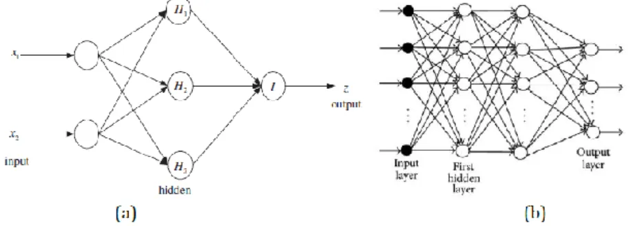
BPNN is a three-layer feed-forward neural network, which includes an input layer, a hidden layer and an output layer with linear neurons (Basheer & Hajmeer, 2000; Örkcü & Bal, 2011; Sermpinis et al., 2012; Upadhyay, Choudhary, & Tripathi, 2011). The typical structure of BPNN is shown in Fig. 1 (a) with one hidden layer and in Fig. 1 (b) with two hidden layers.
Fig. 1: A typical structure of backpropagation architecture (Örkcü & Bal, 2011; Upadhyay et al., 2011).
C. The algorithm of BPNN:
Based-on the BPNN algorithm model, there are four steps involved in building a forecasting algorithm which consists of (1) collecting data; collecting and preparing sample data, (2) data normalization; to train the ANNs more efficiently, (3) training and testing data; to train and test the performance of the model, and (4) comparing the predicted output with the desired output; using statistical analysis, e.g. sum of square error (SSE), mean of square error (MSE), mean of percentage error (MPE), mean of absolute percentage error (MAPE), mean of absolute deviation (MAD), determination (R), and coefficient of determination (R2), (Abhishek, Kumar, Ranjan, & Kumar, 2012; Al Shamisi, Assi, & Hejase, 2011; Ticknor, 2013). Furthermore, the BP training algorithm described below
Step 0: Initiation of all weights
Step 1: If the termination condition is not fulfilled, do step 2-8
Step 2: For each pair of training data, do steps 3-8
Phase 1: Feed forward:
Step 3: Each unit receives input signals and transmitted to the hidden unit above
Step 4: Calculate all the output in the hidden layer units Zj (j = 1,2,…,p)
Step 5: Calculate all the network output in unit output yk (k = 1,2,…,m)
Phase 2: Back propagation:
Step 6: Calculate factor δ output unit based on unit output error yk (k = 1,2,…,m)
tk = output target
Calculate weight change wkj, with the learning rate α
Step 7: Calculate factor δ unit hidden layer based on the error in each hidden layer unit
Factor δ hidden layer unit
Calculate weight change rate vji
Phase 3: Weight modification:
Step 8: Calculate the weight of all the changes that led to the output unit
Weight changes that led to the hidden layer units
2.2. The Construction and Forecast of BPNN Model to Forecast Neural Network: A. BPNN neural network input variables and output variables:
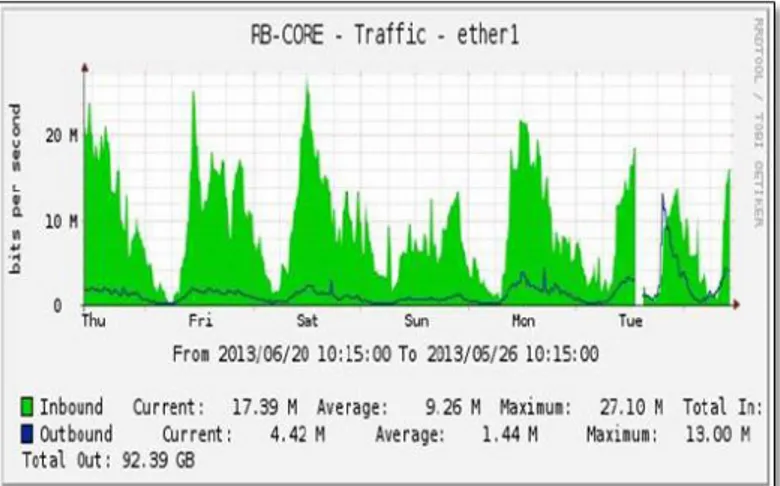
Input variable selection is an important task before the BPNN modeling. In this research, the network traffic data is a collection of daily network user data, Fig 2. Then, each network traffic data was captured by the CACTI software. The testing and training data as input variables are four days network traffic data.
B. Input samples pretreatment:
Before training, the inputs and tests data will be normalized. The normalization aims to get the data with a smaller size that represents the original data without losing its own characteristics. The normalization formula form is:
Where:
X: actual value of samples; Xmax: maximum value; Xmin: minimum value
In this study, four days daily network traffic data from 21 – 24 June 2013 (192 samples series data) was captured. Then, the datasets consist of 144 (90%) samples for data training and 48 (10%) samples for data testing or five neurons, P = [p(t-5),p(t-4),p(t-3),p(t-2),p(t-1)], and the number of output neurons is one, p'(t), as shown in table 1.
Table 1: The daily network data after normalized in 21-24 June 2014.
C. Determining training sample and test samples:
To test the accuracy and efficiency of the network, there are 1 to 144 groups of data selected as the study samples, the 145 to 192 groups as the test samples and using the trained BPNN to predict. The BPNN architecture that has been used consists of two types which are the one-hidden layer and two-hidden layers. Then, the activation function for one-hidden layer; from input to hidden layer was tansig, and from hidden layer to output was purelin. For the two-hidden layers; from input to hidden layers were tansig and logsig, and from hidden layers to output was purelin, then both used gradient descent with momentum (traingdm) algorithms. In this test, the MSE was used to get different values for comparison of actual data and predicted data.
RESULTS AND DISCUSSIONS
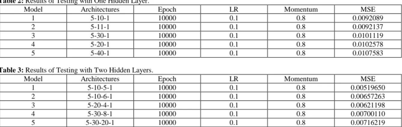
This section presents the best achieved result by the BPNN algorithm with one and two hidden layers. Table 2 and 3 show the computed values of MSE considering different network architectures. The network architectures in the second column of tables 2 and 3 consist of three parts. The first number indicates the number of neurons in the input layer, the second number represents the neurons in the hidden layers, and the last number represents the neurons in the output layer. Then, epochs, learning rate, and momentum have been set are 1000, 0.1, and 0.8.
Table 2: Results of Testing with One Hidden Layer.
Model Architectures Epoch LR Momentum MSE
1 5-10-1 10000 0.1 0.8 0.0092089
2 5-11-1 10000 0.1 0.8 0.0092137
3 5-30-1 10000 0.1 0.8 0.0101119
4 5-20-1 10000 0.1 0.8 0.0102578
5 5-40-1 10000 0.1 0.8 0.0107583
Table 3: Results of Testing with Two Hidden Layers.
Model Architectures Epoch LR Momentum MSE
1 5-10-5-1 10000 0.1 0.8 0.00519650
2 5-10-6-1 10000 0.1 0.8 0.00657263
3 5-20-4-1 10000 0.1 0.8 0.00621198
4 5-30-8-1 10000 0.1 0.8 0.00700110
5 5-30-20-1 10000 0.1 0.8 0.00716219
Training results indicate that the performance goals were not all achieved the desired results, even though the specified epoch has been reached. This means, the network was still not able to recognize a given input pattern. Nevertheless, the resulting graph during training showed a decrease or nearly in the MSE values.
recognizing the pattern. However, when the learning rate value is increased, the MSE value increases. Third, the momentum which has a small value was 0.8. Thus, there has been a decrease in the gradient. Therefore, the
momentum value of 0.8 was set to prevent the phenomena of local minimum.
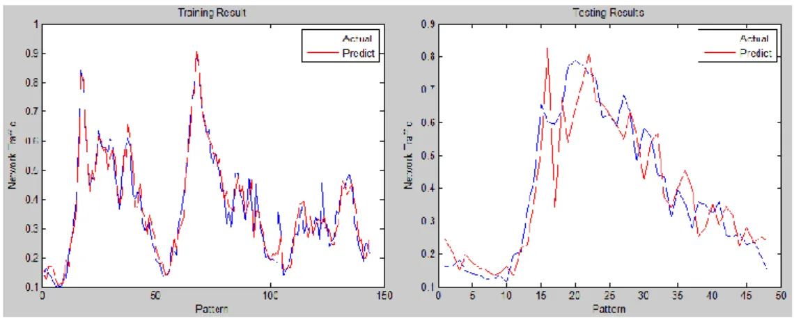
Fig. 3: Graphs of BPNN with 5-10-5-1 Architecture Training and Testing Results.
Despite the fact, the MSE values of both the training are not desired, but these values have been relatively small and approached. From the results of the training that the first training smallest MSE was 0.4604679 with the architecture 5-40-1, and the second training smallest MSE was 0.72413896 with the architecture 5-20-4-1. The settings hidden layer has indicated differences in the MSE values. In the second training, small enough value of learning rate 0.1 has been used. Thus, decrease the gradient has been confirmed. However, the number of iterations has been increased so that, to achieve convergence has needed a long time. But if, added value of the constant learning rate, then, has no gradient decreased significantly.
Therefore, the second training which has two-hidden layer, 5-10-5-1 architecture, epoch 10000, 0.001
performance goals, momentum 0.8, gradient descent algorithm with momentum (traingdm) with the transfer function tansig, logsig from the input layer to the hidden layers and functions transfer, purelin of hidden layers to the output was optimal. The architecture has been able to achieve the performance goals, and also has a pretty good MSE value.
Conclusion:
This paper has presented a daily network traffic prediction method based on BPNN. The performance of the training algorithm can be used to estimate the architectures of the neuron. Based on the results of this research concluded that two-hidden layers or multi-layer algorithm is better than one-hidden layer or single-layer algorithm term of performance. The use of this method provides a new way of thinking for simulating and predicting the usage of daily network traffic of ICT Center, and also provide a reference for the planning of network traffic at Universitas Mulawarman. Therefore, one of the planned future works is to combine the Back propagation method with a genetic algorithm (GA) in order to optimize the prediction accuracy.
REFERENCES
Abhishek, K., A. Kumar, R. Ranjan, S. Kumar, 2012. A Rainfall Prediction Model using Artificial Neural Network. 2012 IEEE Control and System Graduate Research Colloquium (ICSGRC 2012).
Al Shamisi, M.H., A.H. Assi, H.A.N. Hejase, 2011. Using MATLAB to Develop Artificial Neural Network Models for Predicting Global Solar Radiation in Al Ain City – UAE. In A. Assi (Ed.), Engineering Education and Research Using MATLAB: InTech.
Basheer, I.A., M. Hajmeer, 2000. Artificial neural networks: fundamentals, computing, design, and application. Journal of Microbiological Methods, 43: 3-31.
Birdi, Y., T. Aurora, P. Arora, 2013. Study of Artificial Neural Networks and Neural Implants. International Journal on Recent and Innovation Trends in Computing and Communication, 1(4).
Chen, G., K. Fu, Z. Liang, T. Sema, C. Li, P. Tontiwachwuthikul, R. Idem, 2014. The genetic algorithm based back propagation neural network for MMP prediction in CO2-EOR process. Fuel, 126: 202-212. doi: http://dx.doi.org/10.1016/j.fuel.2014.02.034.
Claveria, O., S. Torra, 2014. Forecasting tourism demand to Catalonia: Neural networks vs. time series models. Economic Modelling, 36: 220-228. doi: http://dx.doi.org/10.1016/j.econmod.2013.09.024.
Sermpinis, G., C. Dunis, J. Laws, C. Stasinakis, 2012. Forecasting and trading the EUR/USD exchange rate with stochastic Neural Network combination and time-varying leverage. Decision Support Systems, 54: 316-329. doi: 10.1016/j.dss.2012.05.039.
Ticknor, J.L., 2013. A Bayesian regularized artificial neural network for stock market forecasting. Expert Systems with Applications, 40: 5501-5506. doi: http://dx.doi.org/10.1016/j.eswa.2013.04.013.
Upadhyay, K.G., A.K. Choudhary, M.M. Tripathi, 2011. Short-term wind speed forecasting using feed-forward back-propagation neural network. International Journal of Engineering, Science and Technology, 3(5): 107-112.