EXCHANGE SPATIAL-ENERGY INTERACTIONS
G. А. Korablev
[a]*Keywords: Lagrangian equations; wave functions; spatial-energy parameter; electron density; elementary particles; quarks.
The notion of spatial-energy parameter (P-parameter) is introduced based on the modified Lagrangian equation for relative motion of two interacting material points, and is a complex characteristic of important atomic values responsible for interatomic interactions and having the direct connection with electron density inside an atom. Wave properties of P-parameter are found, its wave equation having a formal analogy with the equation of -function is given. With the help of P-parameter technique, numerous calculations of exchange structural interactions have been performed and the applicability of the model for the evaluation of the intensity of fundamental interactions has been demonstrated. Initial theses of quark screw model are also discussed.
* Corresponding Authors
E-Mail: [email protected]
[a] Department of Physics, Izhevsk State Agricultural Academy
SPATIAL-ENERGY PARAMETER
When oppositely charged heterogeneous systems interact, a certain compensation of the volume energy takes place, which results in the decrease in the resultant energy e.g. during the hybridization of atom orbitals.1 But this is not a direct algebraic deduction of corresponding energies. The comparison of numerous regularities of physical and chemical processes leads us to assume that in such and similar cases the principle of adding reverse values of volume energies or kinetic parameters of interacting structures are observed. For instance, during the ambipolar diffusion, when joint motion of oppositely charged particles is observed in the given medium (in plasma or electrolyte), the diffusion coefficient (D) is found as follows:
𝐷= 1 𝑎+
+ 1 𝑎−
where
а+ and а are the charge mobility of both atoms and η is the constant coefficient.
Total velocity of the topochemical reaction (υ) between the
solid and gas is found as follows:
1 𝑣=
1 𝑣1
+ 1 𝑣2
where
υ1 is the diffusion velocity of the reagent and
υ2 is the velocity of reaction between the gaseous reagent and solid.
Change in the light velocity (Δv) when moving from the vacuum into the given medium is calculated by the principle of algebraic deduction of reverse values of the corresponding velocities:
1 ∆𝑣=
1 𝑣−
1 𝑐
where с is the velocity light in vacuum.
Lagrangian equation for relative motion of the system of two interacting material points with masses m1 and m2 in coordinate х is as follows:
𝑚np𝑥" =
𝜕𝑈
𝜕𝑥 (1)
where
1 𝑚r
= 1 𝑚1
+ 1 𝑚2
(1a)
here U is themutual potential energy of material points, mr is
the reduced mass and х" = а (characteristic of system acceleration).
For elementary interaction areas ∆х, 𝜕𝑈
𝜕𝑥≈ ∆𝑈 ∆𝑥 then
𝑚r𝑎∆𝑥 = −∆𝑈
1 1/(𝑎∆𝑥)×
1 (1/𝑚1+ 1/𝑚2)
≈ ∆𝑈
or
1
1/(𝑚1𝑎∆𝑥) + 1/(𝑚2𝑎∆𝑥)
≈ ∆𝑈
Since in its physical sense the product miaΔx equals the
potential energy of each material point (-∆Ui), then
1 ∆𝑈≈
1 ∆𝑈1
+ 1 ∆𝑈2
Thus the resultant energy characteristic of the interaction system of two material points is found by the principle of adding the reverse values of initial energies of interacting subsystems.
Therefore assuming that the energy of atom valence orbitals (responsible for interatomic interactions) can be calculated by the principle of adding the reverse values of
some initial energy components, the introduction of P
-parameter as the averaged energy characteristic of valence orbitals is postulated based on the following equations.
1 𝑞2/𝑟
i
+ 1 𝑊i𝑛i
= 1 𝑃E
(3)
1
𝑃
0=
1
𝑞
2+
1
(𝑊𝑟𝑛)
i(4)
𝑃E= 𝑃0/𝑟i
(5) here
Wi is the orbital energy of electrons,2
ri is orbital radius of i–orbital,3
q=Z*/n*,4,5
ni is the number of electrons of the given orbital,
Z* and n* are the effective charge of the nucleus and effective main quantum number, and
r is the bond dimensional characteristics.
The term Р0 will be called spatial-energy parameter (SEP),
and e РEas effective Р–parameter (effective SEP). Effective
SEP has a physical sense of some averaged energy of valence electrons in the atom and is measured in the energy units e.g., in electron-volts (eV).
Values of Р0-parameter are tabulated constant values for the electrons of the atom given orbital.
For the dimensionality, SEP can be written as follows:
[𝑃0] = [𝑞2] = [𝐸] × [𝑟] = [ℎ] × [] =
𝑘𝑔 𝑚3
𝑠2 = 𝐽𝑚
where [E], [h] and [] are the dimensionalities of energy, Plank’s constant and velocity respectively.
The introduction of P-parameter should be considered as further development of quasi-classic notions using quantum-mechanical data on the atom structure to obtain the energy conditions criteria of phase-formation. At the same time, for similarly charged systems (e.g. orbitals in the given atom) and homogeneous systems the principle of algebraic addition of these parameters will be preserved.
∑ 𝑃E= ∑(𝑃0/𝑟i) (6)
∑ 𝑃E= ∑ 𝑃0
𝑟 (7)
∑ 𝑃0= 𝑃0′ + 𝑃0′′+ 𝑃0′′′+ ⋯, (8)
𝑟 ∑ 𝑃E= ∑ 𝑃0 (9)
Here P-parameters are summed for the valence orbitals of all
atoms.
To calculate the values of РE-parameter at the given
distance from the nucleus either atomic radius (R) or ionic radius (ri) can be used instead of r depending on the bond type.
Applying the equation (8) to hydrogen atom we can write down the following
𝐾(𝑒 𝑛)1
2= 𝐾(𝑒
𝑛)2
2+ 𝑚𝑐2𝜆
(10)
where е is the elementary charge, n1 and n2 are the main quantum numbers, m is the electron mass, с is the velocity of electromagnetic wave, is the wave length, K is a constant.
Using the known correlations = c/ 𝜆 and 𝜆 = h/mc (where
h is Plank’s constant, is the wave frequency) from the formula (10), the equation of spectral regularities in hydrogen atom can be obtained, in which 2π2е2/hc = K.
EFFECTIVE ENERGY OF VALENCE
ELECTRONS IN AN ATOM AND ITS
COMPARISON WITH THE STATISTIC MODEL
The modified Thomas-Fermi equation, converted to a
simple form by introducing dimensionless variables,6 can be
written as eqn. (11).
𝑈 = 𝑒(𝑉i− 𝑉0+ 𝜏02) (11)
where
V0 is the countdown potential,
е is the elementary charge,
0 is the exchange and correlation corrections,
Vi is the interatomic potential at the distance
ri from the nucleus and
U is the total energy of valence electrons.
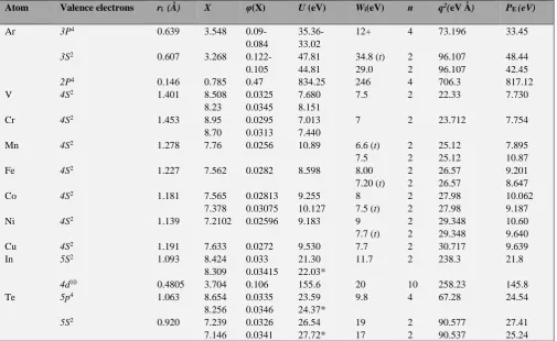
For some elements, the comparisons of the given value U
with the values of РE-parameter are given in Table 1.
As it is seen form the Table 1 the parameter values of U and
РE are practically the same (in most cases with the deviation not exceeding 1-2 %) without any transition coefficients. Multiple corrections introduced into the statistic model are compensated with the application of simple rules of adding reverse values of energy parameters, and SEP quite precisely conveys the known solutions of Thomas-Fermi equation for interatomic potential of atoms at the distance ri from the nucleus. Namely the following equality takes place:
𝑈 = 𝑃E= 𝑒(𝑉i− 𝑉0+ 𝜏02) (12)
Table 1. Comparison of total energy of valence electrons in atom calculated in Thomas-Fermi statistic atom model (U) and with the help of approximation.
Atom Valence electrons ri (Å) X φ(X) U (eV) Wi(eV) n q2(eV Å) PE(eV)
Ar 3P4 0.639 3.548 0.09-
0.084
35.36-33.02
12+ 4 73.196 33.45
3S2 0.607 3.268 0.122-
0.105
47.81 44.81
34.8 (t) 29.0
2 2
96.107 96.107
48.44 42.45
2P4 0.146 0.785 0.47 834.25 246 4 706.3 817.12
V 4S2 1.401 8.508
8.23
0.0325 0.0345
7.680 8.151
7.5 2 22.33 7.730
Cr 4S2 1.453 8.95
8.70
0.0295 0.0313
7.013 7.440
7 2 23.712 7.754
Mn 4S2 1.278 7.76 0.0256 10.89 6.6 (t)
7.5
2 2
25.12 25.12
7.895 10.87
Fe 4S2 1.227 7.562 0.0282 8.598 8.00
7.20 (t) 2 2
26.57 26.57
9.201 8.647
Co 4S2 1.181 7.565
7.378
0.02813 0.03075
9.255 10.127
8 7.5 (t)
2 2
27.98 27.98
10.062 9.187
Ni 4S2 1.139 7.2102 0.02596 9.183 9
7.7 (t) 2 2
29.348 29.348
10.60 9.640
Cu 4S2 1.191 7.633 0.0272 9.530 7.7 2 30.717 9.639
In 5S2 1.093 8.424
8.309
0.033 0.03415
21.30 22.03*
11.7 2 238.3 21.8
4d10 0.4805 3.704 0.106 155.6 20 10 258.23 145.8
Te 5p4 1.063 8.654
8.256
0.0335 0.0346
23.59 24.37*
9.8 4 67.28 24.54
5S2 0.920 7.239
7.146
0.0326 0.0341
26.54 27.72*
19 17
2 2
90.577 90.537
27.41 25.24 Note: (1) Bond energies of electrons Wiare obtained: “t” – theoretically (by Hartry-Fock method), “+” – by XPS method, all the rest – by he
results of optic measurements; (2) “*” – energy of valence electrons (U) calculated without Fermi-Amaldi amendment.
2/3i(3е/5) × (Vi – V0);
2/3i Aе × (Vi – V0 + 20)=[Aе ×ri × (Vi – V0 + 20)]/ri
(13)
where А is a constant.
According to the Eqns. (12) and (13) we have the following correlation (Eqn. 14), setting the connection between Р
0-parameter and electron density in the atom at the distance ri
from the nucleus.
βi
2 3=𝐴𝑃0
𝑟i
(14)
Since in the value 𝑒(𝑉i− 𝑉0+ 𝜏02) in Thomas-Fermi model
there is a function of charge density, Р0-parameter is a direct characteristic of electron charge density in atom.
This is confirmed by an additional check of equality
correctness (14) using Clementi function.7 A good
correspondence between the values of βi calculated via the
value of Р0 and obtained from atomic functions is observed.
Wave equation of
P
-parameter
For the characteristic of atom spatial-energy properties two
types of P-parameters with simple correlation between them
are introduced, PE=P0/R, where R is the dimension
characteristic of the atom. Taking into account additional quantum characteristics of the sublevels in the atom, this
equation in coordinate х can be written down as follows:
∆𝑃E≈
∆𝑃0
∆𝑥
or
𝜕𝑃E≈
𝜕𝑃0
𝜕𝑥
where
the value ΔР equals the difference between Р
0-parameter of i-orbital and
РCD–countdown parameter (parameter of basic state at
the given set of quantum numbers).
According to the established rule8 of adding P-parameters of
∆𝑃"E− ∆𝑃′E= 𝑃E,λ
where РE,λ is the spatial-energy parameter of quantum
transition.
Taking as the dimension characteristic of the interaction
Δλ=Δх, we have
Δ𝑃"0
Δ𝜆 − Δ𝑃′
0
Δ𝜆 = 𝑃0
Δ𝜆 or Δ𝑃′
0
Δ𝜆 − Δ𝑃"0
Δ𝜆 = − 𝑃0𝜆
Δ𝜆
If we divide termwise by , we get
(Δ𝑃
′ 0
Δ𝜆 − Δ𝑃"0
Δ𝜆 ) ∆𝜆 ~
𝑑2𝑃 0
Δ𝜆2
i.e.,
𝑑2𝑃 0
𝑑𝜆2 +
𝑃0
∆𝜆2≈ 0
Taking into account the interactions where 2πΔх = Δλ (closed
oscillator), we have the following equation
𝑑2𝑃 0
𝑑𝑥2 + 4𝜋 2× 𝑃0
∆𝜆2 ≈ 0
then:
, ∆𝜆 = ℎ/𝑚
𝑑
2𝑃 0
𝑑𝑥2 + 4𝜋 2 𝑃0
ℎ2𝑚
2𝜈2≈ 0 or
𝑑
2𝑃 0
𝑑𝑥2 + 8𝜋2𝑚
ℎ2 𝑃0𝐸k = 0 (15)
where Ek=mv2/2electron kinetic energy.
Schrödinger equation for stationary state in coordinate х is
𝑑2𝜓
𝑑𝑥2 + 8𝜋2𝑚
ℎ2 𝜓𝐸k = 0 (16)
Comparing the Eqns. (15) and (16) we can see that Р
0-parameter correlates numerically with the value of function
i.e., P0 and in general it is proportional to it, P0. Taking
into account wide practical application of P-parameter
methodology, we can consider this criterion as the
materialized analog of -function.
Since Р0-parameters, like -function possess wave
properties, the principles of superposition should be executed for them, thus determining the linear character of equations
of adding and changing P-parameters.
Wave properties of
P
-parameters and principles of
their addition
Since P-parameter possesses wave properties (by analogy
with -function) the regularities of the interference of
corresponding waves should be executed mainly with structural interactions.
Minimum interference, oscillation attenuation (in anti-phase), takes place if the difference in wave motion (∆) equals the odd number of semi-waves:
∆
=(
2𝑛 + 1)
𝜆2 = 𝜆
(
𝑛 + 1 2)
,where n = 0, 1, 2, 3, … (17)
As applied to P-parameters this rules means that minimum
interaction occurs if P-parameters of interacting structures are also “in anti-phase” i.e, there is an interaction either between oppositely charged systems or heterogeneous atoms (for example, during the formation of valence-active radicals CH, CH2, CH3, NO2 …, etc).
In this case the summation of P-parameters takes place by
the principle of adding the reverse values of P-parameters as
in Eqns. (3) and (4).
The difference in wave motion (∆) for P-parameters can be
evaluated via their relative value ( = P2/P1) or via the relative difference in P-parameters (coefficient ), which with the minimum of interactions produce an odd number:
𝛾 =𝑃2
𝑃1= (𝑛 +
1
2) = 3
2, 5
2… (18)
when n = 0 (main state), P2/P1 = ½
Let us mention that for stationary levels of one-dimensional
harmonic oscillator the energy of these levels = h(n+½),
therefore in quantum oscillator, in contrast to a classical one, the minimum possible energy value does not equal zero.
In this model the minimum interaction does not produce the zero energy, corresponding to the principle of adding the
reverse values of P-parameters (Eqns. 3 and 4). Maximum
interference, oscillation amplification (in the phase), takes place if the difference in wave motion equals the even number of semi-waves:
∆= 2𝑛𝜆
As applied to P-parameters the maximum amplification of interactions in the phase corresponds to the interactions of similarly charged systems or systems homogeneous in their properties and functions (for example, between the fragments and blocks of complex organic structures, such as CH2 and NNO2 in octogen). Then
𝛾 =𝑃2
𝑃1= (𝑛 + 1) (19)
By the analogy, for “degenerated” systems (with similar values of functions) of two-dimensional harmonic oscillator the energy of stationary states: =h(n+1).
In this model, the maximum interaction corresponds to the principle of algebraic addition of P-parameters (Eqns. 6-8). When n = 0 (basic state) we have Р2 = Р1, or maximum
interaction of structures takes place when their P-parameters
equal. This postulate can be used as the main condition of
isomorphic replacements.8
STRUCTURAL EXCHANGE SPATIAL-ENERGY
INTERACTIONS
In the process of solution formation and other structural interactions the single electron density should be set in the points of atom-component contact. This process is accompanied by the redistribution of electron density between the valence areas of both particles and transition of the part of electrons from some external spheres into the neighbouring ones. Apparently, frame atom electrons do not take part in such exchange.
Obviously, when electron densities in free atom-components are similar, the transfer processes between boundary atoms of particles are minimal, this is favourable for the formation of a new structure. Thus the evaluation of the degree of structural interactions in many cases means the comparative assessment of the electron density of valence electrons in free atoms (on averaged orbitals) participating in the process.
The less is the difference (Р'0/r'i – P"0/r"i), the more favourable is the formation of a new structure or solid solution from the energy point.
In this regard, the maximum total solubility, evaluated via
the coefficient of structural interaction, , is determined by
the condition of minimum value , which represents the
relative difference of effective energies of external orbitals of interacting subsystems:
𝛼 = 𝑃′0⁄ −𝑃"𝑟i′ 0⁄𝑟i"
(𝑃′0⁄ +𝑃"𝑟i′ 0⁄ )/2𝑟i"
100 % (20)
𝛼 =𝑃′S−𝑃"S
𝑃′S+𝑃"S200 % (20a)
where РS, the structural parameter, is found by Eqn. (20).
1
𝑃S =
1
𝑁1𝑃E′ + 1
𝑁1𝑃E"
+ ⋯ (20b)
here N1 and N2 are the number of homogeneous atoms in subsystems.
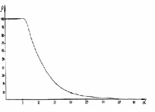
The nomogram of the dependence of structural interaction degree (ρ) on the coefficient α, unified for the wide range of structures was prepared based on all the data obtained. Figure
1 presents such a nomogram obtained using РE-parameters
calculated via the bond energy of electrons (wi) for structural interactions of isomorphic type.
The mutual solubility of atom-components in many (over a thousand) simple and complex systems have been evaluated earlier using this technique. The calculation results are in
compliance with theoretical and experimental data.8
Isomorphism as a phenomenon is used to be considered as applicable to crystalline structures. But similar processes can obviously take place between molecular compounds, where their role and importance are not less than those of purely coulomb interactions.
In complex organic structures during the interactions the main role can be played by separate “blocks” or fragments. Therefore, it is necessary to identify these fragments and evaluate their spatial-energy parameters. Based on the wave properties of P-parameter, the overall P-parameter of each fragment can be found by the principle of adding the reverse values of initial P-parameters of all atoms. The resultant P -parameter of the fragment block or all the structure is
calculated by the rule of algebraic addition of P-parameters
of the fragments constituting them.
The role of the fragments can be played by valence-active
radicals, e.g. СН, СН2, ОН-, NO, NO2, SO42-, etc. In complex
structures the given carbon atom usually has two or three side bonds. During the calculations by the principle of adding the
reverse values of P-parameters, the priority belongs to those
bonds, for which the condition of minimum interference is better performed. Therefore the fragments of the bond С-Н (for СН, СН2, СН3 …) are calculated first, then separately the
fragments N-R, where R is the binding radical (for example –
for the bond C-N).
Apparently spatial-energy exchange interactions (SEI) based on equalizing electron densities of valence orbitals of atom-components have in nature the same universal value as
purely electrostatic coulomb interactions, but they
supplement each other. Isomorphism, known from the time of E. Mitscherlich (1820) and D.I. Mendeleev (1856), is only a particular manifestation of this general natural phenomenon. The numerical side of the evaluation of isomorphic replacements of components both in complex and simple
systems rationally fit in the frameworks of P-parameter
methodology. More complicated is to evaluate the degree of structural SEI for molecular, including organic structures.
The technique for calculating P-parameters of molecules,
But such structures and their fragments are frequently not completely isomorphic with respect to each other. Nevertheless there is SEI between them, the degree of which in this case can be evaluated only semi-quantitatively or qualitatively. By the degree of isomorphic similarity all the systems can be divided into the following three types.
(1) Systems mainly isomorphic to each other i.e., systems with approximately identical number of dissimilar atoms and nearly similar geometrical shapes of interacting orbitals.
(2) Systems with the limited isomorphic similarity i.e, systems which either (a) differ by the number of dissimilar atoms but have nearly similar geometrical shapes of interacting orbitals, or (b) have definite differences in geometrical shapes of orbitals but have identical number of interacting dissimilar atoms.
(3) Systems not having isomorphic similarity i.e., systems, which differ considerably both by the number of dissimilar atoms and geometric shapes of their orbitals.
Then taking into account the experimental data, all types of SEI can be approximately classified as follows.
Systems (1): (i) α 0-6 %, ρ = 100 %. Complete
isomorphism, there is complete isomorphic replacement of atom-components, (ii) 6 % α < 25-30 %, ρ = 98 – (0-3) %. There is either a wide or limited isomorphism according to
nomogram 1. (iii) α 25-30 %, no SEI.
Systems (2): (i) α 0-6 %, (а) there is the reconstruction of chemical bonds, can be accompanied by the formation of a new compound, (b) breakage of chemical bonds can be accompanied by separating a fragment from the initial
structure, but without attachments or replacements. (ii) 6 %
α < 25-30 %, limited internal reconstruction of chemical bonds without the formation of a new compound or
replacements is possible and (iii) α 20-30 %, no SEI.
Systems (3): (i) α 0-6 %, (а) limited change in the type of chemical bonds of the given fragment, internal regrouping of atoms without the breakage from the main part of the
molecule and without replacements, (b) change in some
dimensional characteristics of the bond is possible. (ii) 6 %
α < 25-30 %, very limited internal regrouping of atoms is possible and (iii) α 25-30 %, no SEI.
Nomogram (Figure 1) is obtained for isomorphic interactions for systems of types (1) and (2).
Figure 1. Dependence of the structural interaction degree (ρ) on the coefficient α
In all other cases the calculated values α and ρ refer only to the given interaction type, the nomogram of which can be clarified by reference points of etalon systems. If we take into account the universality of spatial-energy interactions in nature, this evaluation can be significant for the analysis of structural rearrangements in complex biophysical-chemical processes.
Fermentative systems contribute a lot to the correlation of structural interaction degree. In this system the ferment structure active parts (fragments, atoms, ions) have the value of РE-parameter that is equal to РE-parameter of the reaction final product. This means the ferment is structurally “tuned” via SEI to obtain the reaction final product, but it will not induced into it due to the imperfect isomorphism of its structure in accordance with (3).
The most important characteristics of atomic-structural interactions (mutual solubility of components, energy of chemical bond, energetics of free radicals, etc) were
evaluated in many systems using this technique.8-15
TYPES OF FUNDAMENTAL INTERACTIONS
According to modern theories, the main types of interactions of elementary particles, their properties and specifics are mainly explained by the availability of special complex currents e.g., electromagnetic, proton, lepton, etc. Based on the foregoing model of spatial-energy parameter the exchange structural interactions finally come to flowing and equalizing the electron densities of corresponding atomic-molecular components. The similar process is obviously appropriate for elementary particles as well. It can be assumed that in general case interparticle exchange interactions come to the redistribution of their energy masses,
М.
The elementary electrostatic charge associated with the electron as a carrier is the constant of electromagnetic interaction. Therefore for electromagnetic interaction we will calculate the system proton-electron.
For strong internucleon interaction that comes to the
exchange of π-mesons, let us consider the systems
nuclides-π-mesons. Since the interactions can take place with all three
mesons (π-, π0 and π+), we take the averaged mass in the
calculations (<М> = 136,497 МeV s-1).
Rated systems for strong interaction are
Р - (π-, π0, π+), (Р-n) - (π-, π0, π+)
and
(n-P-n) - (π-, π0, π).
Neutrino (electron, muonic) and its antiparticles were considered as the main representatives of weak interaction.
Dimensional characteristics of elementary particles (r)
were evaluated in femtometer units (1 fm= 10-15 m) by the
At the same time, the classic radius, re=e2/mes2, was used for electron, where e is the elementary charge, me is the electron mass and s is the speed of light in vacuum. The
fundamental Heisenberg length (6.690 10-4 fm) was used as
the dimensional characteristic of weak interaction for neutrino.16
The gravitational interaction was evaluated via the proton
P-parameter at the distance of gravitational radius (1.242 10-39 fm).
In the initial eqn. (3) for free atom, Р0-parameter is found
by the principle of adding the reverse values q2 and wr, where
q is the nucleus electric charge, w is the bond energy of the
valence electron. Modifying the Eqn. (3), as applied to the interaction of free particles, we receive the addition of reverse values of parameters Р = Мr for each particle by Eqn. (21).
1/ Р0=1/(Мr)1 + 1/(Мr)2+ (21)
where М is the energy mass of the particle (MeV s-2).
By using Eqn. (21) and the earlier data,16P0-parameters of
coupled strong and electromagnetic interactions were
calculated in nuclides-π-mesons (Рn-parameters and
proton-electron , Рe-parameter).
For weak and gravitational interactions only the parameters
Рυ = Мr and Рr = Мr were calculated, as in accordance with the Eqn. (21), the similar nuclide parameter with greater value does not influence the calculation results.
The relative intensity of interactions (Table 2) was found by the equations for the following interactions.
Strong αB=< 𝑃n>/𝑃n>= 𝑃n⁄𝑃n= 1 (22а)
Electromagnetic 𝛼B= 𝑃e⁄< 𝑃n>= 1 136.983⁄ (22b)
Weak 𝛼B= 𝑃e⁄< 𝑃n>,
α
B=
2.04 10-10, 4.2 10-6 (22c)Gravitational 𝛼B= 𝑃e⁄< 𝑃n>= 5.9 × 10−39 (22d)
In the calculations for αв, the value of Рn-parameter was multiplied by the value equaled 2π/3, i.e. <P>=(2π/3)Pn. Number 3 for nuclides consisting of three different quarks is “a magic” number (see the next section for details). As it is known, number 2π has a special value in quantum mechanics and physics of elementary particles. In particular, only the value of 2π correlates theoretical and experimental data when evaluating the sections of nuclide interaction with each other.17
As it has been reported,18 nuclear interactions are
distinguished as very strong, strong and moderately strong. For all particles in the large group with relatively similar mass values of mass, unitary multiplets or supermultiplets, very strong interactions are similar.18 In the frames of the given model a very strong interaction between the particles
corresponds to the maximum value of P-parameter, Р = Мr
(coupled interaction of nuclides). Taking into consideration the equality of dimensional characteristics of proton and
neutron, by eqn. (21), we obtain the values of Рn-parameter
as 401.61; 401.88 and 402.16 (МeVfm s-2) for coupled
interactions p-p, p-n and n-n, respectively, thus obtaining the
average value αB = 4.25. It is a very strong interaction. For
eight interacting nuclides αB ≈ 1.06 i.e., a strong interaction.
When the number of interacting nuclides increases, αB
decreases – moderately strong interaction. Since the nuclear
forces act only between neighbouring nucleons, the value αB
cannot be very small.
The expression of the most intensive coupled interaction of nuclides is indirectly confirmed by the fact that the life period of double nuclear system appears to be much longer than the characteristic nuclear time.19
Thus it is established that the intensity of fundamental interactions is evaluated via Рn-parameter calculated by the principle of adding the reverse values in the system nuclides-π-mesons. Therefore, it has the direct connection with Plank’s constants.
(2π/3)Pn≈ Er = 197.3 МeVfms-2 (23)
(2π/3)Pт≈ Mnλk= 197.3 МeVfms-2 (23а)
where
Е and r, Plank’s energy and Plank’s radius are
calculated via the gravitational constant,
Мn, λk, energy mass and nuclide Compton wave-length.
In Eqn. (21), the exchange interactions are evaluated via the initial P-parameters of particles equaled to the product of mass by the dimensional characteristic i.e., P = Мr.
Since these Р-parameters can refer to the particles
characterizing fundamental interactions, their direct
correlation defines the process intensity degree (αB):
𝛼𝐵= 𝑃𝑖
𝑃𝑛=
(𝑀𝑟)𝑖
(𝑀𝑟)𝑛 (24)
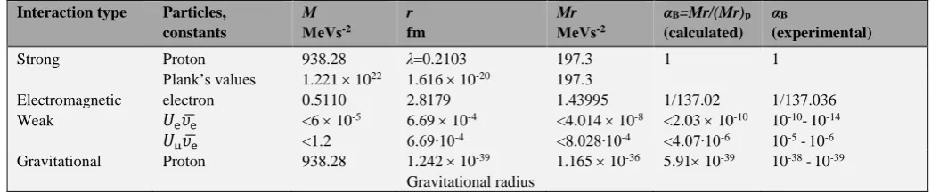
The calculations by the Eqn. (24), using the known Plank’s values and techniques are given in table 3. As before, the energy and dimensional characteristics are taken from the literature.16
The results obtained are in accordance with theoretical and experimental data.20,21
ON QUARK SCREW MODEL
Let us proceed from the following theses and assumptions:
(i) By their structural composition macro- and micro world resemble. One part has some similarity with the other: solar system – atom – atom nucleus – quarks.
Table 2. Types of fundamental interactions
Table 3. Evaluation of the intensity of fundamental interactions using Plank’s constants and parameter P = Mr.
Interaction type Particles, constants
М
МeVs-2
r
fm
Мr
МeVs-2
αB=Mr/(Mr)p
(calculated)
αB
(experimental)
Strong Proton 938.28 λ=0.2103 197.3 1 1
Plank’s values 1.221 1022 1.616 10-20 197.3
Electromagnetic electron 0.5110 2.8179 1.43995 1/137.02 1/137.036
Weak 𝑈e𝜐̅e <6 10-5 6.69 10-4 <4.014 10-8 <2.03 10-10 10-10-10-14
𝑈μ𝜐̅e <1.2 6.69∙10-4 <8.028∙10-4 <4.07∙10-6 10-5 -10-6 Gravitational Proton 938.28 1.242 10-39
Gravitational radius
1.165 10-36 5.91 10-39 10-38 -10-39
(iii) Main property of all systems is motion, translatory, rotary and oscillatory.
(iv) Description of these motions can be done in Euclid three-dimensional space with coordinates x, y and z.
(v) Exchange energy interactions of elementary particles
are carried out by the redistribution of their energy mass M
(МeVs-2).
Based on these theses we suggest discussing the following screw model of the quark.
(i) Quark structure is represented in certain case as a spherical one, but in general quark is a flattened (or elongated) ellipsoid of revolution. The revolution takes place
around the axis (х) coinciding with the direction of angular
speed vector, perpendicular to the direction of ellipsoid deformation.
(ii) Quark electric charge (q) is not fractional but is an integer, but redistributed in three-dimensional space with its virtual concentration in the directions of three coordinate axes. Each axis having an electric charge = q/3.
(iii) Quark spherical or deformed structure has all three types of motion. Two of them, rotary and translator, are in accordance with the screw model, which beside these two motions, also performs an oscillatory motion in one of three mutually perpendicular planes, xoy, xoz, yoz (Figure 2).
(iv) Each of these oscillation planes corresponds to the symbol of quark color, e.g. red for xoy, blue for xoz and green for yoz.
(v) Screw can be “right” or “left”. This directedness of screw rotation defines the sign of quark electric charge. Let us assume that the left screw corresponds to positive and right to negative quark electric charge.
(vi) Total number of quarks is determined by the following scheme: for each axis (x, y and z) of translator motion two screws (right and left) with three possible oscillation planes.
(vii) We have 3 2 3 = 18 quarks. Besides, there are 18
antiquarks with opposite characteristics of screw motions. In all there are thus 36 types of quarks.
These quark numbers can be considered as realized degrees of freedom of all three motions (3 translatory + 2 rotary + 3 oscillatory).
Translatory motion is preferable by its direction, coinciding with the direction of angular speed vector. Such elementary particles constitute our World. The reverse direction is less preferable, this is “Antiworld”.
Motion along axis х in the direction of the angular speed vector, perpendicular to the direction of ellipsoid deformation, is apparently less energy consumable and corresponds to the quarks U and d, forming nuclides.
Interac-tion type
М, <М>
МeVs-2
r
fm
Elementary particles
М, <М>
МeVs-2
r
fm
Pn, Pe, Pν,Pg
МeVfms-2
2/3Pn=
<Pn>
αB , <αB>
(Eqn. 22)
αB
(experi-mental)
Electro-magnetic
Р 938.28 0.856 e- 0.5110 2.8179 P
e=1.4374 - 1/136.983 1/137.04
Strong Р 938.28 0.856 π-, π0, π+ 136.497 0.78 P
n=94.0071 196.89 1 1 P-n 938.92 0.856 π-, π0, π+ 136.497 0.78 P
n=94.015 196.90 1 1
n-P-n 939.14 0.856 π-, π0, π+ 136.497 0.78 P
n=94.018 196.91 1 1
Weak
υ
e, 𝜐̅𝑒 <6 10-5
6.69 10-4
Pν=4.014∙10-8 <2.04
10-10
10-10 -10-14
υ
μ, 𝜐̅𝑒 <1.2 6.69 10-4Pν=8.028 10
-4
<4.2 10-6 10-5 -10-6
Gravitati-onal
P 938.28 1.242
10-39
Pг=1.17 10
-36
5.9 10-39
Such assumption is in accordance with the values of energy masses of quarks in the composition of andirons, 0.33. 0.33, 0.51, 1.8, 5 in GeVs-2 for d, u, s, c, b, t types of quarks, respectively.
The quark screw model can be proved by other calculations and comparisons also.
Figure 2. Structural scheme of quark in section yoz.
CALCULATION OF ENERGY MASS OF FREE
NUCLIDE (TAKING NEUTRON AS AN
EXAMPLE)
Neutron has 3 quarks d1-u-d2 with electric charges 1, +2, -1, distributed in three spatial directions, respectively. Quark
u cements the system electrostatically. Translatory motions of
the screws d1-u-d2 proceed along axis х, but oscillatory ones proceed in three different mutually perpendicular planes (Pauli principle is realized).
Apparently, in the first half of oscillation period u-quark oscillates in the phase with d1-quark, but in the opposite phase
with d2-quark. In the second half of the period everything is
vice versa. In general such interactions define the geometrical equality of directed spatial-energy vectors, thus providing the so-called quark discoloration.
The previously formulated rules of adding P-parameters
spread to both types of P-parameters (Р0 and РE). In this case,
there is an additional energy РE-parameters, since the
subsystems of interactions possess similar dimensional characteristics. As both interactions are realized inside the overall system, РE-parameters are added algebraically, and more accurately, in this case, geometrically by the following formula
𝑀
2 =
√
𝑚12+ 𝑚 2 2
where, M is the energy mass of free neutron, m1 = m2 = 330
МeVs-2 masses of quarks u and d (in the composition of androns).
The calculation gives M = 933.38 МeVs-2. This is for strong interactions. Taking into account the role of quarks in
electromagnetic interactions,21 we get the total energy mass
of a free neutron as M=933.38+933.38/137=940.19 МeVs-2.
With the experimental value M = 939.57 МeVs-2 the relative
error in calculations is 0.06 %.
CALCULATION OF BOND ENERGY OF
DEUTERON VIA THE MASSES OF FREE
QUARKS
The particle deuteron is formed during the interaction of a free proton and neutron. The bond energy is usually calculated as the difference of mass of free nucleons and mass of a free deuteron. Let us demonstrate the dependence of deuteron bond energy on the masses of free quarks. The quark masses are added algebraically in the system already formed, in proton m1 = 5 + 5 + 7 = 17 МeVs-2, in neutron m2 = 7 + 7
+ 5 =19 МeVs-2. As a dimensional characteristic of deuteron
bond we take the distance corresponding to the maximum value of nonrectangular potential pit of nucleon interaction. By the graphs experimentally obtained we know that such distance approximately equals 1.65 fm. Exchange energy interactions of proton and neutron heterogeneous systems are evaluated based on the Eqn. (21). Then we have:
1/ (MC1.65 K) = 1/(17∙0.856) + 1/(19∙0.856),
where K = 2π/3. Based on the calculations we have MC=
2.228 МeVs-2, this practically coincides with reference data20 (MC = 2.225 МeVs-2).
After modification, the basic theses of quark screw model can be applied to other elementary particles (proton, electron, neutron, etc) also. For instance, an electrically neutral particle neutron can be considered as a mini-atom, the analog of hydrogen atom.
CONCLUSIONS
(1) The notion of spatial-energy parameter (P-parameter) is
introduced based on the simultaneous accounting of important atomic characteristics and modified Lagrangian equation.
(2) Wave properties of P-parameter are found, its wave equation formally similar to the equation of ψ-function is obtained.
(3) Applying the methodology of P-parameter
(а) most important characteristics of exchange energy interactions in different systems have been calculated
(b) intensities of fundamental interactions have been calculated and
(c) initial theses of quark screw model have been given.
y
z
REFERENCES
1Batsanov, S. S., Zvyagina, R. A., Overlap integrals and challenge
of effective charges, Novosibirsk, Nauka, 1966, 386.
2Fischer, C. F., Atomic Data Nucl. Data Tables, 1972, 4, 301-399. 3Waber, J. T., Cromer, D. T., J. Chem. Phys., 1965, 42 (12),
4116-4123.
4Clementi, E., Raimondi, D. L., J. Chem. Phys., 1963, 38 (11),
2686-2689.
5Clementi, E., Raimondi, D. L., J. Chem. Phys., 1967, 47 (4),
1300-1307.
6Gombash, P., Atom statistic theory and its application, М., 1951,
398.
7Clementi, E., J. B. M. S. Res. Develop. Suppl., 1965, 9 (2), 76. 8Korablev, G. A., Spatial Energy Principles of Complex Structures
Formation, Leiden, Brill Academic Publishers and VSP, Netherlands, 2005, 426.
9Korablev, G. A., Kodolov, V. I., Lipanov, А. М., Chem. Phys.
Mesoscopy. 2004, 6, 5-18.
10Korablev, G. A., Zaikov G. E., J. Appl. Poly. Sci., 2006, 101,
2101-2107.
11Korablev, G. A., Zaikov, G. E., Reactions and Properties of
Monomers Polymers, Nova Science Publishers, Inc., New York, 2007, 203-213.
12Korablev, G. A., Zaikov, G. E., Success Gerontol., 2008, 21 (4),
535-563.
13Korablev, G. A., Zaikov, G. E., Mechanics of composition
materials and constructions, 2009, 15 (1), 106-118.
14Korablev, G. A., Zaikov, G. E., Chem. Phys., RAS, М.: 2006, 25
(7), 24-28.
15Korablev, G. A., Zaikov, G. E., Monomers, Oligomers, Polymers,
Composites and Nanocomposites Research, Nova Science Publishers, USA, 2008, 441-448.
16Murodyan, R. M., PEChAYa, М., Atomizdat., 1977, 8 (1), 175-192. 17Barashenkov, V. S., Sections of interactions of elementary
particles, Nauka, Moscow, 1966, 532.
18Yavorsky, B. M., Detlav, А. А., Reference-book in physics, Nauka,
Moscow, 1968, 940.
19Volkov, V. V., PEChAYa, М., Atomizdat., 1975, 6, 1040-1104. 20Bukhbinder, I. L., Sorov Educ. J., 1997, 5,
http://nuclphys.sinp.msu.ru /mirrors/fi.htm.
21Okun, L. B., Weak interactions,
http://www.book-site.ru/fulltext/1/001/008/ 103/ 116.htm.