THE ADVANCED COMPUTING SYSTEMS ASSOCIATION
The following paper was originally published in the
Proceedings of the Workshop on Intrusion Detection
and Network Monitoring
Santa Clara, California, USA, April 9–12, 1999
A Statistical Method for Profiling Network Traffic
David Marchette
Naval Surface Warfare Center B10
© 1999 by The USENIX Association All Rights Reserved
Rights to individual papers remain with the author or the author's employer. Permission is granted for noncommercial reproduction of the work for educational or research purposes. This copyright notice must be included in the reproduced paper. USENIX acknowledges all trademarks herein.
For more information about the USENIX Association: Phone: 1 510 528 8649 FAX: 1 510 548 5738 Email: [email protected] WWW: http://www.usenix.org
A Statistical Method for Profiling Network Traffic
David Marchette
Naval Surface Warfare Center B10
Dahlgren, VA 22448
[email protected]
Abstract
Two clustering methods are described and applied to network data. These allow the clustering of machines into “activity groups”, which consist of machines which tend to have similar activity profiles. In addition, these methods allow the user to determine whether current activity matches these profiles, and hence to determine when there is “abnormal” activity on the network. A method for visualizing the clusters is described, and the approaches are applied to a data set consisting of a months worth of data from 993 machines.
1. Introduction
The task of monitoring the traffic on a large network is a daunting one. At a minimum, one needs to filter out all the “normal” or “uninteresting” traffic in order to focus attention on those connections that are unusual or indicative of potential problems. The problem ad-dressed in this work is the one of characterizing “nor-mal” traffic, and recognizing and flagging “abnor“nor-mal” traffic.
At one level, “abnormal” can refer simply to those connection attempts that are considered undesir-able and hence are disallowed by the firewall. Once a suspicious connection attempt has been detected, the traffic from that source can be pulled and perused to determine if allowed connections may have been used successfully to compromise the network.
The problem with this approach is that it can only catch those things one already knows about. Every network administrator has a bad ports list and a bad IPs list, and any connection matching one of these lists is scrutinized. However, some connections are only bad if they are to certain machines, but are perfectly normal to others. For example, one may allow individuals to set up ftp servers, provided they follow certain guidelines to ensure relative security. So one may see a fair amount of ftp traffic in and out of the network to a (pe-riodically changing) subset of machines. Suppose a machine that has never had ftp traffic suddenly starts to get ftp connections. An alert network manager might
want to check to make sure that the system administra-tor for that machine has intended to set up an externally available ftp site, rather than someone taking advantage of a misconfiguration or vulnerability. This can be par-ticularly important if the machine in question is an in-frastructure machine, contains sensitive information, or is otherwise an important target for attackers. In fact, any traffic that is “unusual” for a give machine or class of machines should be flagged for further analysis.
The problem then is to determine what is “normal” and hence what is “unusual” for the network. This paper will describe two techniques based on some statistical approaches to clustering and discrimination. The techniques will be described and an example for a large (nearly 1000 machine) network will be provided.
The data considered in this work consists of six fields: date/time, source IP address,
source port, destination IP address, destination port, and protocol (TCP or UDP). These data can be obtained through programs such as netlogger or tcpdump. Other information, such as SYN/ACK flags, packet size etc. can easily be incorporated within the basic framework described herein. The data consist of a subset of the external connections to our network for the months of March and April 1998. The subset of the data chosen comprised those machines that had at least 10 connec-tion attempts to at least two distinct ports in the month of April. Only those connection attempts in which the source was external to our network and the destination was internal were considered. The month of April was used to define “normal” activity, and the data from March was used to obtain performance statistics. The availability of reported attacks during the month of March, and the fact that we had done considerable analysis of the April data set dictated this choice.
2. Measuring Network Traffic
The first and most obvious way to measure network activity is to keep count of the number of accesses to each port within a given time period (hourly, daily, etc.). When the count for a port on a given machine or set of machines is unusually high, this is an indication
of a potential problem. The determination of what con-stitutes “unusually high” can be made through studying the normal fluctuations of these quantities in historical data.
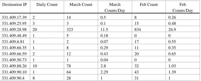
Table 1 shows one way of utilizing counts to monitor a network. The incoming telnet sessions are tabulated for the current day and compared with the activity for the previous two months. These are real data collected on our network. Obviously the IP ad-dresses have been changed. The analyst can scan a list such as this for daily counts that exceed the normal for the previous months, pull the traffic to that machine to determine who is making these connections, and, if warranted, pull additional traffic for the appropriate machines. Obviously this kind of analysis can only be done for a relatively small number of ports and ma-chines, but for some of the most obvious services this can provide the analyst with considerable information about the traffic on the network.
The above idea can be extended to allow the consideration of all the ports in a natural way, by nor-malizing the counts by the overall traffic, thus obtain-ing a probability estimate, instead of a “connections per day” measure. So now one has an estimate of the prob-ability of having an access to any given port for any given machine. This can then be used as above to de-termine whether the traffic for a given time period is abnormal, or it can provide feedback for individual accesses. Port access attempts which have a low prob-ability can be flagged as unusual and worthy of further investigation.
These ideas can be extended to consideration of “sessions”, or sequential accesses from a single source IP. There are at least two approaches here. One can count sessions in much the same manner as above,
and flag low probability sessions as unusual. This is essentially the approach taken by Forrest et al [3]. Or one can model the sessions (for example as a Markov chain) and flag a session that deviates from the model. Work in this area is ongoing and we will not consider these ideas further in this paper.
Once again it is important to remember that these methods are not designed to catch intruders by themselves, but rather to filter the traffic to eliminate from consideration that which is obviously “normal”. Experience has shown that on a network of hundreds to thousands of machines, with millions of connections a day, events with very low probabilities happen quite frequently, far too frequently to be dealt with on an individual basis (assuming the usual number of security personnel reviewing the log files).
2. Clustering Machines by Network
Activ-ity
The above method works well when dealing with a small number of machines. Once the number of ma-chines on the network rises into the hundreds, one would like to aggregate machines into “activity types”. Intuitively, one would imagine that machines with similar functions should have similar normal activity. This is the case, although ones intuition as to which machines should be similar may not be entirely accu-rate. The idea is to do this aggregation in an automated manner. In the statistics literature this type of aggrega-tion is called “clustering”.
One of the most widely used clustering meth-ods is the k-means method. This requires knowledge of the number of clusters in the data. Once one has
Table 1: Telnet access counts
Destination IP Daily Count March Count March Counts/Day
Feb Count Feb Counts/Day 331.409.17.39 2 14 0.5 8 0.26 331.409.25.95 3 3 0.1 15 0.48 331.409.28.98 20 323 11.5 834 26.9 331.409.48.49 1 5 0.18 0 0 331.409.6.81 1 2 0.07 17 0.55 331.409.66.35 1 8 0.29 11 0.35 331.409.66.59 2 12 0.43 20 0.65 331.409.50.73 1 1 0.04 0 0 331.409.88.26 10 78 2.8 32 1.03 331.409.90.10 1 64 2.29 43 1.39 331.409.90.4 8 28 1 31 1
decided how many clusters are represented within the data, the algorithm proceeds as follows:
Algorithm: k-means
0. Initialize the k cluster centers (for example at k randomly chosen data points)
1. While the clusters change do 1.1 - 1.2 1.1 Determine (via a nearest distance calcula-tion) which data belong to which cluster. 1.2 Recompute (via the mean) the cluster cen-ters.
2. Return the clusters.
The algorithm is simple to implement and works quite well in most situations. Note that there are a couple of issues that need to be addressed. First, one must decide on the number of clusters in the data. There is no easy answer as to how to do this. Typically it is done by visualizing the data, and through guess work. Once one has decided on the value of k one must pick starting centers for the clusters. This can be done via visualization of the data if the dimension is low enough for this to be practical, or through trial-and-error.
To illustrate the k-means method, the data has been reduced as follows: counts were kept for the first 1024 ports in both TCP and UDP, and a separate count is kept for all ports above 1024, again both for TCP and UDP. These counts are then normalized by the overall amount of traffic to produce a probability vector of size 2050 (1024+1+1024+1). These vectors will be referred to as “activity vectors”. 993 machines were considered in the example. Obviously 993 2050-dimensional vec-tors would task most visualization techniques to the breaking point. The method we use is to plot the data as an image, with the pixel values corresponding to the port-probabilities. Even this is difficult to display on a typical computer screen. The data has been further re-duced by eliminating from the display those ports with a probability of less than 0.2. This results in vectors of length 61 for these data.
Figure 1 shows the results of a k-means clus-tering with the number of clusters set at 10 (arbitrarily). The cluster centers were initialized at random. The dif-ferent images correspond to the difdif-ferent clusters (a cluster containing a single machine is not shown). Each row corresponds to a machine, while each column cor-responds to the probability vector, color coded for dif-ferent probability values. It is clear from this figure that the clusters are distinct, and most of them are fairly homogeneous.
One uses these clusters as follows: all the ma-chines within a cluster are aggregated in the sense that all their data are used to produce an activity vector for
that group. These vectors are then used to classify indi-vidual connections to one of the machines within a given cluster according to their probabilities.
One problem with this approach is that there are some clusters which are not homogeneous, for ex-ample the fourth cluster in the figure. Clusters like this tend to be catch-alls where machines that don’t fit any other cluster criterion are put. Rather than place a hard classification for each machine, it could be noted that some machines appear to fit well with several clusters, and use partial assignments. These could then be used to produce, for example, a weighted average of the ac-tivity vectors, which would better indicate the connec-tion probabilities. While this can be done within the k-means clustering scheme, it is more natural in the scheme which we now describe.
The k-means clustering method could be thought of in terms of estimating the structure (or prob-ability density) of the data via a mixture of “clumps”. These clumps, in the k-means framework are spherical, and could be taken to be normal distributions. One could then use the wide literature on fitting mixture models (see, for example, McLachlan and Basford [4]). Unfortunately, fitting normal mixtures to 2050-dimensional data is simply not possible, without very serious constraints, which essentially reduce the model down to the k-means model. Typically what one does in these situations is reduce the dimension of the data through a projection, and then construct the model within the projected space. This is the approach taken here.
We utilize a method of Cowen and Priebe (see [1] and [2]), called approximate distance clustering (ADC). The idea is to select out a subset of the data, referred to as the witness set. For each data point, de-termine the distance to each element of the witness set and retain the smallest distance. This is the value to which that point gets projected. Thus we are projecting from 2050 dimensional space to 1 dimension. The method can be extended to utilize several witness sets, in which case the projecting dimension is the number of witness sets.
Algorithm: ADC
0. Initialize the witness set (for example select k randomly chosen data points)
1. For each point determine the distances to each point in the witness set
2. Return the smallest of the distances.
Once one has projected the data, one con-structs a normal mixture model estimate of the density of the data. The clusters then become determined by the components of the mixture: each cluster consists of
those points whose posterior probability is highest for the cluster’s component. This allows a natural method for giving partial cluster assignments: use the posterior probabilities.
A mixture model is a weighted sum of normal densities. The weights (called mixing coefficients or proportions) are constrained to be positive and sum to one. The formula for an m-component mixture model is: , 1 ) , , ( ) (
∑
= = i i v i x i x f π ϕ µwhere the iπ correspond to the mixing coeffi-cients, iµ the means, and iv the variances.
As in the k-means method, most mixture model algorithms require the user to decide on the number of components in advance. We use a method that simultaneously estimates the number of compo-nents and the component parameters, which is de-scribed in Priebe et al [5]. The clusters chosen by this method are shown in Figure 2.
Algorithm: AKMDE
0. Start with a single component with mean and variance chosen from the data.
1. While a stopping criterion is not met (for example AIC) do 1.1-1.3
1.1 Construct a nonparametric estimate (kernel estimator) using the current mixture
1.2 Add a new term where the two models dif-fer most.
1.3 Estimate the new model parameters 2. Return the mixture.
The basic idea of the AKMDE algorithm is as follows: one uses a nonparametric (kernel) estimator of the density to test whether the parametric model is ade-quate, and if not, a term is added. So, one uses the mixture to construct the “best” nonparametric estimator that one can, assuming the mixture to be correct. The two estimators are then compared. If the kernel esti-mator is significantly different than the mixture, then a new term is placed where the difference is greatest, and the new mixture model is constructed. This continues until the mixture matches the kernel estimator suffi-ciently closely.
The details of the AKMDE are beyond the scope of this paper. The interested reader is urged to check out the paper for more details.
Figure 3 shows the mixture model constructed on the ADC projected data. The top curve shows the overall density, while the bottom curve shows the mixture model. The x-axis represents the means of the
components while the y-axis represents the mixing co-efficient. The bar at each point represents one standard deviation on either side of the mean. The figure indi-cates that there are basically four to five obvious clus-ters. Figure 2 treats each component as a single cluster, rather than trying to combine components into clusters in this manner. The clusters displayed in Figure 2 are ordered by their means in the same manner as the com-ponents displayed on the bottom of Figure 3. The small component with a mean near 0.7 contains no machines and thus does not appear in the cluster picture.
3. Results
The data for the month of March 1998 was run through the k-means and ADC/AKMDE clusters, assigning to each record a probability. There were 1,757,206 rec-ords. There were a total of 27 source IPs which were determined to be attackers against one or more of the 993 machines in the data set. These consist of only those attacks that could have been detected via these methods. For example, while accesses from certain foreign countries to our facility may have been consid-ered attacks, these were not included in the data unless the attack was detected without consideration of the source. These kinds of attacks can easily be detected by resolving the source IP.
We define attacks very broadly to include any information gathering that might indicate future attacks. An example of this kind of information gathering is using traceroute to determine the routes to our network, and hence the potential bottlenecks which could be attacked to deny service. While traceroutes are a legiti-mate and useful tool, we want to know about them to determine whether they show a pattern over time, which might indicate potential future attacks.
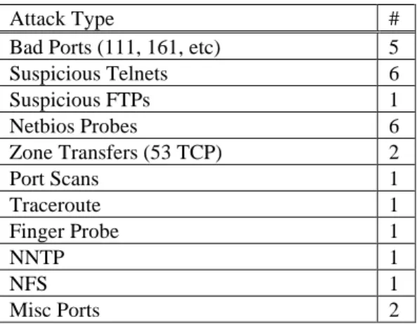
Table 2: Attacks
Attack Type #
Bad Ports (111, 161, etc) 5 Suspicious Telnets 6 Suspicious FTPs 1 Netbios Probes 6 Zone Transfers (53 TCP) 2 Port Scans 1 Traceroute 1 Finger Probe 1 NNTP 1 NFS 1 Misc Ports 2
The attacks considered here are grouped into 11 basic categories as shown in Table 2. Since the techniques described here work on individual access attempts, the attacks are denoted by the service or ac-cess which best describes the attack. Note that two of the attacks, the traceroute and the port scan, are not single port accesses, and yet they are still easily de-tected using this approach, as will be seen below.
The port scan was an unusual one which ap-peared to be looking for services above the usual 1024 range, and so might have been hard to detect using the approach implemented here. Recall that we only con-sider the first 1024 ports individually, grouping all other ports into a “big port” range. Obviously one could extend this approach to include more ports if desirable. Note also that a port scan is defined in terms of a se-quence of access attempts rather than any individual one, and so this method is not the method of choice for detecting these scans.
With that said, it is of interest to note that the scan was easily detected, since the machine scanned had seen very little activity beyond the first 1024 ports.
Port scans that focus only on commonly accessed ports will not be picked up via this method. Clearly, tech-niques that take into account the number of different ports accessed are more appropriate for detecting gen-eral port scans.
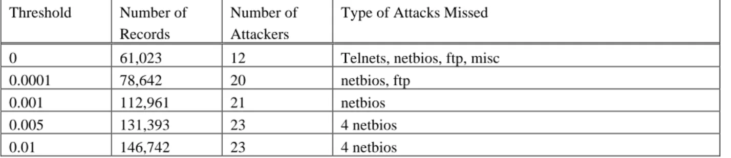
The data are reduced by setting a threshold on the probability and filtering out (ignoring as “normal”) all records with probability exceeding the threshold. The results for several thresholds are given in Tables 3-5. Each table indicates the threshold probability, the number of records that are flagged at or below that probability, the number of attacker IPs which remain in the data to be detected via further processing, and the type of attacks that were missed at that threshold. Table 3 presents the results for the individual machines. This effectively treats each machine as a cluster and uses the activity vector for that machine to determine the prob-ability for the access attempt. Tables 4 and 5 present the results for the two clustering techniques described above. All thresholds in the tables are the same to allow comparisons at a given threshold. Figure 4 shows a plot of these results for various thresholds, plotting number of records against the number of attacks detected.
Table 3: Results on March Test Data: Unclustered Results
Threshold Number of Records
Number of Attackers
Type of Attacks Missed
0 50,217 21 1 Telnet, 2 netbios, ftp, nfs, 1 misc 0.0001 50,288 22 1 Telnet, 2 netbios, nfs, 1 misc 0.001 54,069 23 2 netbios, nfs, 1 misc
0.005 58,962 23 2 netbios, nfs, 1 misc 0.01 63,410 23 2 netbios, nfs, 1 misc
Table 4: Results on March Test Data: ADC Results
Threshold Number of Records
Number of Attackers
Type of Attacks Missed
0 17,069 9 Telnets, netbios, news, ftp, finger, tracerout, misc 0.0001 60,975 13 Telnets, netbios, news, ftp
0.001 108,529 14 Telnets, netbios, ftp 0.005 140,435 23 3 netbios, ftp
Table 5: Results on March Test Data: k means Results
Threshold Number of Records
Number of Attackers
Type of Attacks Missed
0 61,023 12 Telnets, netbios, ftp, misc 0.0001 78,642 20 netbios, ftp
0.001 112,961 21 netbios
0.005 131,393 23 4 netbios
0.01 146,742 23 4 netbios
This is a fairly significant reduction in the amount of data to be processed. When eliminating 90% of the data the ADC method still detects all of the at-tacks. It is important to stress again that these tech-niques should be thought of as data filters. Other intru-sion detection algorithms must be applied to the filtered data to detect the actual attacks. Also, these techniques can only detect abnormal traffic. If a machine or group of machines normally have a certain amount of traffic to a given port, this technique is not designed to detect an unauthorized connection to that port. Other tech-niques, and often other data sources, must be utilized to detect these kinds of attacks.
One strength of this approach is that it does not require a network security expert to implement it, nor does it require perfectly clean (attack free) data. Assuming the undetected attacks in the training data are rare, they will not have too great an effect on the sys-tem. With that said, the performance does degrade if the training data does include attacks.
An interesting point to note is that the individ-ual machine results were not uniformly better than the cluster results. Consider in Figure 4 the point at which each method first detects all the attacks. The ADC method is superior under this metric. Intuitively, one would think that this should not be the case. The reason for this counterintuitive result is as follows. Imagine that a machine was attacked in April but the attack went undetected. This machine then would have a number of access attempts to a port which should have been flagged as abnormal but were left in the training set, thus increasing the probability associated with that port. This can cause new accesses to that port on that ma-chine to be considered “normal” for thresholds below this probability. Now imagine that the machine is clus-tered with others. Presumably these machines did not all have access to this forbidden port, which forces the probability of access to be reduced. One now considers these accesses to be “abnormal”.
This does not come without penalty. If the clusters are not perfectly homogeneous, “normal” ports
may be given lower probabilities than they should have, due to the fact that different machines have (slightly) different access patterns. This results in the superior performance of the individual machine method in the low thresholds. It gets far more attacks than the others do while passing fewer “abnormal” packets.
One issue in these approaches is the time re-quired to implement them. There are two issues here. The first is the time required to generate the statistics. This is highly dependent on the size of ones network and the number of connections that are typically seen to the network. The calculation of these statistics on our class B network takes less than a minute for two months worth of data, in part because of the design of the database. Since this is done once a month, or at most once a week, this is not an unreasonable compu-tational burden.
The second issue is the time required assigning a probability to a new connection and deciding if it is “abnormal” or not. First the statistics for the destination host must be retrieved from the database in which these are stored, then a table lookup provides the probability associated with the destination port. Finally, the prob-ability is compared with the threshold to determine if the connection is to be classed as “abnormal”. All of this can be done in real time or near real time on most networks, particularly if care is taken to optimize the retrieval and look-ups.
If one uses one of the clustering methods the time is essentially the same, the savings comes in the storage requirements. First one determines which clus-ter the host is associated with, then the statistics for the cluster are retrieved and the processing is the same from there on.
4. Future Issues
It is not obvious that the distance measure used in both the k-means and ADC algorithms, Euclid-ean distance, is the appropriate one for these data. It would be of interest to consider other distances with an
eye toward encoding domain specific information into the process. This would allow a more natural method for encoding unregistered ports, for example handling the ranges of ports used in ftp traffic and traceroutes.
The ADC method relies on projecting the data to a lower dimensional space. It would be interesting to consider projections to 2-, 3-, and higher dimensions. Also, the ADC can be coupled with the k-means rather than using the AKMDE. All these are areas of current research.
Time can be taken into account through the consideration of pairs, triples, etc., of connections. These can be clustered in the same manner as above, by constructing probability vectors associated with their frequency. The clustering methods could then be ap-plied to these vectors. More thought will be required when one takes into account both incoming and outgo-ing connections to produce a description of an entire session.
Another issue that must be addressed is the updating of the clusters. As new machines are acquired, old machines are retired or change their function, the clusters must be updated to reflect the new environ-ment. One way to do this is to utilize a sliding window. Every week (or appropriate time unit) the statistics are updated by considering only those records within a recent window of time which were not flagged as at-tacks or as otherwise suspicious activity. This must be done with care to avoid a gradual shift caused by incor-porating missed attacks in the statistics.
As mentioned above, the approach should be fairly robust to incorporation of missed attacks in the training data. One possible approach to eliminating these from the data is to incorporate outlier detection algorithms into the process. One problem with this is the high dimensional nature of the data. It remains to be seen whether missed attacks remain outliers when the data is projected via the ADC or other projection meth-ods.
Much more extensive tests are needed to de-termine the best way to utilize these ideas. The optimal choice of the number of clusters is a difficult problem. Ultimately one must decide if it is necessary to cluster the machines into a small number of clusters instead of treating each machine as an individual. The latter should provide better accuracy while the former can require substantially fewer computations on a large network. The work described here is the first step to answering these questions.
References
[1] Cowen, L.J. and Priebe, C.E., “Randomized Non-linear Projections Uncover High Dimensional Struc-ture”, Advances in Applied Mathematics, Vol. 9, pp. 319-331, 1997.
[2] Cowen, L.J. and Priebe, C.E., “Approximate Dis-tance Clustering”, Computing Science and Statistics”, Vol. 29, pp. 337-346, 1997.
[3] Forrest, S., Hofmeyr, S., and Somayaji, A., “Com-puter immunology”, Communications of the ACM, Vol. 40, No. 10, pp. 88-96, 1997.
[4] McLachlan, G.J., and Basford, K.E., Mixture
Mod-els: Inference and Applications to Clustering, Marcel
Dekker, 1988.
[5] Priebe, C.E., Marchette, D.J., and Rogers, G.W., “Alternating Kernel and Mixture Models”, The Johns Hopkins University Department of Mathematical Sci-ences Technical Report #574, 1997.
Figure 1: Clusters generated by the k-means algorithm. Each rectangle corresponds to a cluster. The x-axis corresponds to port number, while the y-axis corresponds to individual machines. Only those ports that have a probability above 0.2 for some machine are shown, for a total of 61 ports. The probabilities are indicated by gray scale value, with black corresponding to a probability close to 1.
Figure 3: The mixture model generated on the ADC projected data using the AKMDE. The top plot shows the mixture density, while the bottom plot indicates the mixture components. Components are plotted as a point at the mean and mixing coefficient, with a bar indicating one standard deviation on either side of the point.
Figure 4: Results for the three methods under a number of thresholds. The x-axis shows the percentage of packets that are flagged as “abnormal”. The y-axis indicates the number of attacks that remain in the “abnormal” data.