Risk analysis of annuity conversion options in a stochastic mortality environment

(1)

Risk analysis of annuity conversion

options in a stochastic mortality

environment

Alexander Kling, Jochen Ruß und Katja Schilling

Preprint Series: 2012 - 12

Fakultät für Mathematik und Wirtschaftswissenschaften

UNIVERSITÄT ULM

(2)

Risk analysis of annuity conversion options in a stochastic

mortality environment

Alexander Kling

Institut für Finanz- und Aktuarwissenschaften Helmholtzstraße 22, 89081 Ulm, Germany phone: +49 731 5031242, fax: +49 731 5031239

[email protected] Jochen Ruß

Institut für Finanz- und Aktuarwissenschaften and Universität Ulm Helmholtzstraße 22, 89081 Ulm, Germany

phone: +49 731 5031233, fax: +49 731 5031239 [email protected]

Katja Schilling∗

Graduiertenkolleg 1100, Universität Ulm Helmholtzstraße 22, 89081 Ulm, Germany phone: +49 731 5031085, fax: +49 731 5031188

[email protected] October 18, 2012

Abstract

While extensive literature exists on the valuation and risk management of financial guarantees embedded in insurance contracts, both, the corresponding longevity guarantees as well as interactions between financial and longevity guarantees are often ignored. The present paper provides a framework for a joint analysis of finan-cial and longevity guarantees and applies this framework to different annuity conversion options in deferred unit-linked annuities. In particular, we analyze and compare different versions of so-called guaranteed annuity options (GAO) and guaranteed minimum income benefits (GMIB) with respect to the value of the option and the resulting risk for the insurer. Furthermore, we examine whether and to what extent the insurance company is able to reduce the risk by typical risk management strategies. The analysis is based on a combined stochastic model for both, the financial market as well as future survival probabilities. We show that different annuity conversion options have significantly different option values and that different risk management strategies lead to a significantly different risk for the insurance company.

Keywords: financial risk, longevity risk, guaranteed annuity option, guaranteed minimum income benefit, val-uation and risk analysis of embedded guarantees

(3)

1 Introduction

In a pure unit-linked deferred annuity, premiums are typically accumulated in one or several funds until some retirement date at which the policyholder can either receive the account value as a lump sum or convert it into an annuity at then prevailing annuity rates. The resulting annuity payments depend on the fund value at the policyholder’s retirement date and on then prevailing interest rates and mortality expectations (which determine the conversion rate). In particular, at the start of the deferment period such contracts do not guarantee a minimum annuity amount. Therefore, insurance companies often add certain guarantees to deferred unit-linked annuity contracts in order to increase customer acceptance. Furthermore, in some countries (e.g. in Germany), certain guarantees are even required to qualify for tax advantages.

For these reasons, a variety of different forms of annuity guarantees within unit-linked deferred an-nuities are being offered in many markets worldwide. Typically, such guarantees constitute complex embedded options with a payoff that depends on the development of the underlying fund, interest rates, and mortality. Nevertheless, these guarantees can differ significantly with respect to both, their value at the start of the deferment period and their ‘character’, i.e. the question whether they are predominantly equity, interest or mortality options. As experienced in the UK during the late 1990s, such options (due to long contract terms of commonly several decades) can become unexpectedly valuable and a potential cause for an insurer’s insolvency (cf. Boyle and Hardy, 2003).

In this paper, we consider three different types of annuity conversion options. The first one, the guaranteed annuity option (GAO), guarantees the policyholder at the start of the deferment period a certain minimum conversion rate that will be applied at the end of the deferment period to convert the account value into a lifelong annuity. The second option is a limited GAO. It reduces the insurer’s risk by defining a maximum account value up to which the guaranteed conversion factor at most applies. Any fund value above this amount can only be annuitized at then prevailing rates. The third option type, a so-called guaranteed minimum income benefit (GMIB), is often offered within variable annu-ities in the US. This option guarantees the policyholder at the start of the deferment period a minimum amount for the lifelong annuity which is, in particular, independent of the development of the fund value. With this guarantee, at the retirement date the policyholder can choose between receiving the guaranteed annuity, converting the account value into a lifelong annuity at then prevailing rates, and taking the account value as a lump sum.

We use a combined stochastic financial and mortality model to analyze the value of and the risk re-sulting from these three annuity conversion options for insurance companies. We particularly consider the effect of different risk management strategies.

During the last decade, several authors have addressed the valuation of GAOs. For example, Boyle and Hardy (2003), Ballotta and Haberman (2003), and Van Haastrecht et al. (2010) derive explicit formulas for the market price of GAOs. In particular, Van Haastrecht et al. (2010) assume stochastic volatility for the equity price and apply a one-factor as well as a two-factor Gaussian interest rate model in order to compare the resulting GAO prices. However, the above authors’ analytical approach is only possible when we assume deterministic survival probabilities and then interpret GAOs as call options on coupon bonds.

Meanwhile, there seems to be a broad consensus that the future development of mortality cannot be forecast with sufficient precision and thus needs to be modeled stochastically, too (cf. Currie et al., 2004). Thus, among others, Milevsky and Promislow (2001), Biffis and Millossovich (2006), Ballotta and Haberman (2006) (which is an extension of Ballotta and Haberman, 2003), and Schrager (2006) not only model equity and interest rates as stochastic processes, but they also project future survival probabilities by means of so-called spot force models in order to adequately price GAOs. There

(4)

also exists some literature on the valuation of GMIBs, commonly in the general context of pricing guarantees within variable annuities, as e.g. Bauer et al. (2008b), Marshall et al. (2010), and Bacinello et al. (2011).

However, in order to assess the insurer’s risk implied by annuity conversion options such as GAOs and GMIBs, knowing the option’s value is not sufficient, in particular, when the corresponding risks cannot be completely hedged. Therefore, an analysis of the risk associated with annuity conver-sion options in a stochastic model that combines the financial market as well as mortality seems worthwhile. In our paper, we analyze the insurer’s risk and examine whether and to what extent the insurance company is able to reduce the risk by risk management strategies typically used in prac-tice. In our combined stochastic financial and mortality model, the financial market is modeled by a one-factor Cox-Ingersoll-Ross model for the interest rates and a geometric Brownian motion for the fund value, while for projecting the survival probabilities a slightly modified version of the forward mortality model proposed by Bauer et al. (2008a) is used.

The remainder of this paper is organized as follows. In Section 2, we specify the combined financial and mortality model. Section 3 introduces the insurance contract and the considered annuity conver-sion options, as well as the considered risk management strategies and risk measures. In Section 4, we present the results of our numerical analyses including several sensitivity analyses. Finally, Section 5 summarizes and concludes.

2 Financial market and mortality model

For the remainder of this paper we fix a finite time horizon T∗ and a filtered probability space (Ω,F,_F,_P) with _F = (Ft)0≤t≤T∗ satisfying the usual conditions of right-continuity and _P

-completeness. Throughout, Ft describes the total information available at time t. We assume F0

to be trivial and setF =FT∗.Additionally, all processes introduced below are assumed to be adapted

and of bounded variation. In what follows, we introduce the two components of our stochastic model: the financial market and the mortality model.

2.1 Financial market

We consider a financial market where the only primary tradeable assets are a bank account, zero coupon bonds with any maturityT ∈[0, T∗],and a fund. We assume that trading takes place contin-uously, without any transaction costs or spreads, and all assets are assumed to be perfectly divisible.

The bank accountB(t)evolves according to the differential equation

dB(t) = r(t)B(t)dt, B(0) = 1,

wherer(t)denotes the short rate at timet.Following Cox et al. (1985), the_P-evolution of the short rate is modeled as a mean-reverting square root process

dr(t) =κ(θ−r(t))dt+σr p

r(t)dWr(t), r(0)>0,

with _P-Brownian motion (Wr₍_t₎₎

0≤t≤T∗. The parameters κ, θ and σ_r are positive constants, κ

de-scribing the speed of mean reversion,θthe long-run mean level, andσrthe volatility. For2κθ ≥σr2,

the short rate remains strictly positive.

In Section 2.3 we specify our choice of risk-neutral measure _Q such that the _Q-dynamics of (r(t))0≤t≤T∗ again follow a square-root diffusion with risk-neutral parametersκ˜, θ˜and σ˜_r.

(5)

page 66) P(t, T) = A(t, T)e−B(t,T)r(t), 0≤t ≤T ≤T∗, whereA(t, T) = 2he(˜κ+h)(T −t) 2 2h+(˜κ+h)(eh(T−t)₋₁₎ 2˜κ ˜ θ ˜ σ2r , B(t, T) = 2(e h(T−t)₋₁₎ 2h+(˜κ+h)(eh(T−t)₋₁₎, andh= p ˜ κ2_{+ 2˜}_σ2 r.

The fund value process(S(t))0≤t≤T∗ follows a slightly modified geometric Brownian motion with

P-dynamics

dS(t) = (λS+r(t))S(t)dt+σSS(t)dWS(t), S(0)>0.

Compared to a standard geometric Brownian motion the drift is not constant, but given by the F-adapted process µ(t) = λS + r(t), 0≤t≤T∗, where λS denotes the equity risk

pre-mium. Again, σS > 0 is the volatility and (WS(t))0≤t≤T∗ a _P-Brownian motion. Let the

pa-rameter ρ ∈ [−1,1] characterize the correlation between Wr and WS. Then, by means of a _P -Brownian motion(WS∗₍_t₎₎

0≤t≤T∗independent of(Wr(t))₀_≤_t_≤_T∗,we can specifyWS(t) =ρWr(t)+

p

1−ρ2_WS∗₍_t₎_{, t} _∈_[0_{, T}∗_]_.

Note that later on we are only interested in the fund value at maturityT,

but not in the whole path in between. Thus, it seems sufficient to choose this rather simple fund value process.

2.2 Mortality model

We consider a homogeneous portfolio of policyholders aged x at time 0. Let τ_xi ∈ (0, T∗], i∈_N,

denote the random residual lifetime of the i-th policyholder as seen from time 0. All residual life-times are modeled as_F-stopping times. In the following, we distinguish between the information on the financial market and the death probabilities on the one hand, and the information on the actual occurrence of death on the other hand. Both information flows are modeled by strict subfiltrations

GandI ofF,respectively, and we assume that F = G∨I,i.e., Ft = Gt∨ It for allt ∈ [0, T∗].In

particular, the survival information_Iis given byIt=W_i∈_NIti, t∈[0, T∗],where

Ii

t =σ{1{τi

x≤s},0≤s≤t}

is the smallest filtration with respect to whichτi

x is a stopping time.

In the following, all equalities between random variables are in the almost sure sense. We as-sume that the residual lifetimes are conditionally independent and identically distributed given the

σ-algebraGT∗.The conditional independence implies that once the information on the environment

carried by _Gis taken into account, the residual randomness in the residual lifetimes is independent across individuals (cf. Biffis et al., 2010, p. 288). The assumption of identically distributed random variables givenGT∗ implies that for alli, j ∈_N

EP P τxi ≤t GT∗Gs = EP P τxj ≤t GT∗Gs ,

and by the tower property of conditional expectations we get

P τxi ≤t G_s =_P τ_xj ≤tG_s (2.1) for anys, t∈[0, T∗].Both assumptions, the conditional independence as well as the conditional iden-tical distribution, are quite natural. In particular, it directly follows that{1{τi

x>t}, i∈N}, t ∈[0, T

∗_]_,

(6)

A conditional version of Kolmogorov’s strong law of large numbers then yields (cf. Majerek et al., 2005, p. 154) 1 n n X i=1 1{τi x>t} P-a.s. −−→_P τ_x1 > tG_T∗ (n→ ∞). (2.2)

Finally, we come back to the filtration _F. It can be shown that for all i ∈ _N (cf. Bielecki and Rutkowski, 2004, p. 145) P τxi > T Ft =1{τi x>t} P(τxi > T| Gt) P(τxi > t| Gt) . (2.3)

Definingτx :=τx1,equation (2.1) implies thatP(τxi ≤t| Gs) = P(τx ≤t| Gs)for alli ∈ N.Thus,

it is sufficient to solely model the random probabilities_P(τx > T| Gt), t, T ∈ [0, T∗]. For this, we

use a so-called forward mortality model which provides at any future timeta forward mortality table considering any maturityT such that nested simulations can be avoided later on. In addition, such a model implicitly allows for changes in the future mortality trend expectation since it becomes random, too. We follow Börger (2010) and apply a slightly modified version of the forward mortality model introduced by Bauer et al. (2008a) and Bauer et al. (2010), and refer to it as the BBRZ model. In the following, we require that the forward force of mortality with maturityT as from timetfor a person agedxat time0,

µ(t, T, x) :=− ∂

∂T logP(τx > T| Gt), (2.4)

is well defined. Then the BBRZ model assumes that, for any fixed (T, x), the _P-dynamics of the process(µ(t, T, x))0≤t≤T∗ are given by

dµ(t, T, x) = α(t, T, x)dt+σ(t, T, x)dWµ(t), µ(0, T, x)>0, (2.5) where α(t, T, x) denotes the drift, σ(t, T, x) a 6-dimensional volatility vector and (Wµ₍_t₎₎

0≤t≤T∗

a 6-dimensional _P-Brownian motion. We assume that Wµ _{is independent of} _Wr _and _WS∗ _which

corresponds to the assumption that mortality and the financial market are independent. The drift term

α(t, T, x)has to satisfy the condition (cf. Bauer et al., 2008a, p. 176)

α(t, T, x) =σ(t, T, x)

Z T t

σ(t, s, x)>ds, (2.6)

so thatα(t, T, x)is already implicitly given by the volatility structureσ(t, T, x).Furthermore, from definition (2.4) it directly follows

P(τx > T| Gt) = e−

RT

0 µ(t,u,x)du,

which, inserting the dynamics (2.5), yields

P(τx > T| Gt) = e− RT 0 (µ(0,u,x)+ Rt 0α(s,u,x)ds+ Rt 0σ(s,u,x)dWµ(s))du _(2.7) =_P(τx > T)e− RT 0 ( Rt 0α(s,u,x)ds+ Rt 0σ(s,u,x)dW µ₍_s₎₎_du .

This implies that for determining the probabilities _P(τx > T| Gt), t, T ∈ [0, T∗], we actually do

not have to specify the forward forces of mortality. Instead, given (2.6), it is sufficient to know the volatility structure σ(t, T, x) and the best estimate survival probabilities _P(τx > T) at time0. The

volatility structure as suggested by Börger (2010) is given in Appendix A. The best estimate survival probabilities are taken from the generational life table DAV 2004 R (cf. Deutsche Aktuarvereinigung (DAV), 2005).

(7)

2.3 Change of measure

Assuming the absence of arbitrage, we can find a probability measure_Qwhich is equivalent to_Pand under which all discounted price processes are martingales. Since the biometric risk is not tradeable in our financial market, the market is incomplete and the risk-neutral measure_Qis not unique (for a further discussion, cf. Møller and Steffensen, 2007, p. 147).

Letγ(t) = (γr(t), γS∗(t), γ_µ(t)), 0≤t≤T∗,be a_G-adapted process of bounded variation. Define

L(t) = exp − Z t 0 γ(u)dW(u)− 1 2 Z t 0 kγ(u)k2du , whereW(t) := Wr₍_t₎_{, W}S∗₍_t₎_{, W}µ₍_t₎>>

is a_P-Brownian motion by definition, and assume

EP exp 1 2 Z T∗ 0 kγ(u)k2du <∞,

that is, Novikov’s condition is satisfied. Then,_Qdefined by its Radon-Nikodym derivativedQ

dP =L(T

∗₎

is a_P-equivalent probability measure on(Ω,F)(cf. Shreve, 2004, p. 33/34), and by Girsanov’s theo-rem, the processfW(t) =

f Wr₍_t₎_, f WS∗₍_t₎_, f Wµ₍_t₎>>_{defined as} f W(t) = W(t) + Z t 0 γ(u)>du (2.8)

is a_Q-Brownian motion. In particular, the components Wfr(t), WfS

∗

(t) andWfµ(t)are again

inde-pendent Brownian motions now underQ.This implies that the independence of the financial market

and mortality is preserved under_Q.Note that by our choice ofγ we implicitly assume that the mar-ket is risk-neutral with respect to unsystematic mortality risk which is motivated by the law of large numbers (cf. equation (2.2)).

Now we need to specifyγ(t)such that_Qis also a martingale measure. Imposing the restriction

γS∗(t) = 1 p 1−ρ2 λS σS −ρ γr(t)

guarantees that (_BS(₍t_t)₎)0≤t≤T∗ is a _Q-martingale (cf. Graf et al., 2010, p. 25). However, neither the

discounted price process of B(t)nor ofP(t, T)imply additional conditions. Thus, we chooseγr(t)

and γµ(t) under practical aspects. In order to preserve the square-root process of the short rate

un-der_Q,we assumeγr(t) = λr p

r(t), λr ∈R,as proposed e.g. by Brigo and Mercurio (2006, p. 65).

Altogether, this results in the following_Q-dynamics ofr(t)andS(t):

dr(t) = ˜κ(˜θ−r(t))dt+σr p r(t)dfWr(t), r(0) >0, dS(t) = r(t)S(t)dt+σSS(t)dfWS(t), S(0) >0, whereWfS(t) =ρWfr(t) + p 1−ρ2 f WS∗₍_t₎_{, t}_∈_[0_{, T}∗_]_,_and_κ_˜₌_κ₊_λ rσr, θ˜= _κ₊κθ_λ_r_σ_r.A possible

approach for specifying γµ(t) is provided in Bauer et al. (2010, p. 141/142). Instead of explicitly

definingγµ(t), they assume a time-constant Sharpe ratioλµ∈Rand deduce that

(8)

The choice of this rather simple risk process is motivated by the fact that there is still no information available on the structure of the market price of longevity risk.

Finally, risk-neutral survival probabilities_Q(τx > T| Gt), t, T ∈[0, T∗],can be derived from their

P-counterparts as follows. SinceQis equivalent toP, the convergence from (2.2) also holds underQ.

Thus, the conditional dominated convergence theorem (cf. Koralov and Sinai, 2007, p. 182) yields

EQ 1 n n X i=1 1{τi x>t} GT∗ ! Q-a.s. −−−→_P(τx > t| GT∗) (n → ∞). (2.9)

Since the residual lifetimes are assumed to be identically distributed given GT∗ under _P,this holds

under_Qas well, and the left-hand side of (2.9) no longer depends onn.Thus, we obtain

Q(τx > t| GT∗) = lim n→∞E Q 1 n n X i=1 1{τi x>t} GT∗ ! (2.9) = _P(τx> t| GT∗) _Q-a.s. (2.10)

for allt ∈ [0, T∗].The risk-neutral survival probabilities can now be calculated via (cf. Bauer et al., 2010, p. 141) Q(τx > T| Gt) (2.10) = EQ₍ P(τx > T| GT∗)| G_t) (2.7) = (2.8)E Q_e−R0T(µ(t,u,x)+ Ru t α(s,u,x)ds+ Ru t σ(s,u,x)dWfµ(s))du Gt × eR0T Ru t σ(s,u,x)γµ(s)dsdu = EP_e−R0T(µ(t,u,x)+ Ru t α(s,u,x)ds+ Ru t σ(s,u,x)dW µ₍_s₎₎_du Gt × eR0T Ru t σ(s,u,x)γµ(s)dsdu =_P(τx > T| Gt)e RT 0 Ru t σ(s,u,x)γµ(s)dsdu, sinceWfµ(t) =Wµ(t) + Rt

0 γµ(u)duis aQ-Brownian motion andσ(t, T, x) = 0for anyt > T.Note

that the equations actually hold for any deterministic choice ofγµ(t).

3 Liability framework

3.1 General setup of the insurance contracts

We consider different unit-linked deferred annuities that are issued at timet = 0to the homogeneous portfolio of x-year-old policyholders introduced in Section 2.2. At inception of each contract, the policyholder pays a single premium P0 which is invested in a fund with unit value S(0) at time

t= 0. We assume that the policyholder neither pays additional premiums nor makes withdrawals or surrenders during the term of the contract. For the sake of simplicity, we also ignore any ongoing fees associated with the annuity contract. Denoting the policyholder’s account value at timetbyA(t),this implies thatA(t) = A(0)S_S₍₀₎(t) as long as the money is invested in the fund. In case of pre-retirement death, the beneficiaries receive the entire current account value and the contract is terminated.

The deferment period ends with the policyholder’s retirement at time T. The policyholder then has the choice between taking the current account valueA(T)as a lump sum, annuitizing it at then prevailing rates, or choosing a guaranteed annuity by exercising an annuity conversion option. Since the first two alternatives have the same value, in what follows we only consider the choice between

(9)

the account valueA(T)and the guaranteed annuity. The difference between the considered contracts are the guaranteed annuities. They vary from contract to contract and thus define different annuity conversion options as described in more detail in Section 3.2. With respect to the policyholder’s choice, we always assume a financially rational behavior which means that the annuity conversion options are exercised if and only if they are in the money. Besides, all annuities are paid annually in advance throughout the remaining lifetime of the insured.

In addition to the option types, we consider different pricing and hedging strategies of the insurance company. We distinguish whether the insurance company charges a fee for the annuity conversion option or not and whether the fee, if any, is used for hedging or just invested into a bank account (see Section 3.3). Finally, in Section 3.4 we specify the option values and the quantity on which our risk analyses are based, namely the insurer’s loss.

3.2 Annuity conversion options

Before we specify the considered annuity conversion options, we determine the time-T value of an immediate lifelong annuity starting at timeT and paying the policyholder an annuity of unit amount annually in advance. Assuming some finite limiting ageω≤T∗beyond which survival is not possible (a.s.), i.e.0< τx ≤ω−x,the risk-neutral valuation approach yields an annuity value of

EQ   ω−(x+T)−1 X k=0 e−RTT+kr(s)ds1_{_τ x>T+k} FT   = ω−(x+T)−1 X k=0 P(T, T +k)_Q(τx > T +k| FT) =1{τx>T} ω−(x+T)−1 X k=0 P(T, T +k)Q(τx> T +k| GT) Q(τx > T| GT) =:1{τx>T}a(T).

The first equation follows from the assumption that the financial market is independent of mortality and the second equation from the analog to equation (2.3) under_Q. Note that, aside from the indi-cator function which indicates the survival until timeT, this annuity value is almost surely the same for every policyholder of the homogeneous portfolio. Thus, it is sufficient to consider a(T)whose distribution is implied by the models introduced in Section 2.

Guaranteed annuity option (GAO)

A guaranteed annuity option gives the policyholder the right to annuitize the account valueA(T)at some conversion rate g which is already specified at the very beginning of the contract, that is, at time 0. The conversion rate describes the annual annuity guaranteed per unit of the account value. Consequently, the guaranteed life annuity amounts to gA(T) per year. The GAO’s maturity value which is equal to the payoff of an option to exchangeA(T)for an annuity worthgA(T)a(T)is then given by

VGAO(T) := max{gA(T)a(T)−A(T),0}=gA(T) max

a(T)−1

g,0

,

(10)

GAO with limit (Limit)

Since the payoff of the GAO at timeT is proportional to the account valueA(T),the potential loss is unbounded. Therefore, many insurers introduce an upper boundLto which the conversion rateg

at most applies. If A(T) ≤ L, the GAO with limit is identical to the traditional GAO. However, if

A(T)> L,the conversion rateg only applies toLand the resulting annuity is given bygLper year. Any excessA(T)−Lis annuitized at then prevailing rates which is equivalent to paying the additional cash amountA(T)−Lat maturity. Then, analogously to the GAO’s maturity value, we obtain for the time-T value of the GAO with limit

VLimit(T) :=gmin{A(T), L}max

a(T)−1

g,0

,

provided the policyholder is still alive at timeT.Otherwise, the payoff is again just zero.

Guaranteed minimum income benefit (GMIB)

Compared to a GAO, a GMIB does not guarantee a conversion factor on some account value but a fixed minimum annuity instead. Usually, the minimum guaranteed annuity is communicated to the policyholder by defining a guaranteed account value Gand a guaranteed conversion rateg. The guaranteed annuity is then given by gG per year. In other words, the policyholder has the choice between taking out the ‘real’ account value A(T) and choosing an annuity of annual amount gG

which results from annuitizing the ‘virtual’ account valueGat a rate ofg.In case the policyholder is still alive, this implies a time-T option value of

VGMIB(T) := max{gGa(T)−A(T),0}.

Otherwise, the option payoff is again zero. Note that here, in contrast to GAO and GAO with limit, the minimum annuity amount is already nominally known at inception of the contract.

3.3 Insurer’s pricing and hedging strategies

Similar to the option types, we focus on risk management strategies that are commonly used in prac-tice. As observed, some annuity conversion options are offered without any additional charge and no special risk management actions are taken. Sometimes, an option fee is charged, but the contracts are still not adequately hedged. Finally, sometimes option fees are used to buy certain hedge instruments against market risks. These observations result in the following three strategies which are summarized in Table 1:

No hedging Hedging

No option fee A –

Option fee B C

Table 1: Overview of the strategies.

• Strategy A: No option fee, no hedging

The insurer charges no fee for the annuity conversion option. Naturally, since no fee is charged, the insurer does not hedge its option liabilities.

(11)

• Strategy B: Option fee, no hedging

The insurer charges an option fee. Nevertheless, the insurer does not hedge its liabilities. The charged option fee is simply invested in the bank account.

• Strategy C: Option fee, hedging

Again, the insurer charges an option fee. Now the fee is used for hedging the option liabilities against the financial risk during the deferment period.

We assume that any option fee F0 is directly deducted from the single premium P0. Thus, the

policyholder’s initial account value can be generally specified asA(0) = P0−F0,whereF0 = 0 in

the case of strategy A. Later on, the option fee will vary between the different option types and risk management strategies. As a result, the account value and thus the option’s payoff at timeT depend on the option type and the risk management strategy as well. Henceforth, if the context requires, this dependence is indicated by a pair(o, s),whereo∈ {GAO,Limit,GMIB}ands∈ {A,B,C}.

In practice, standard actuarial approaches are typically used for pricing the annuity conversion options (if they are priced at all, i.e. only under strategies B and C). Thus, we derive the option feesF0 charged under strategy B and C assuming deterministic mortality. Uncertainty about future

mortality is simply considered by applying safety margins to best estimate mortality tables, while the financial market is modeled stochastically as in Section 2.1. In contrast, the ‘real’ option value

V(0) as described in Section 3.4 is calculated considering both a stochastic financial market as well as stochastic mortality.

Moreover, since there exists no liquid financial market for longevity instruments, the insurer is only able to hedge its liabilities against the financial risk. In practice, again, the remaining mortality risk is typically taken into account by using mortality tables including safety margins. Therefore, we assume that the insurer’s hedging approach under strategy C is specified assuming deterministic mortality. In Section 4, we analyze the resulting risk under a stochastic mortality model.

In what follows, we assume that the same mortality table is used for pricing and hedging. Lettpˆx

denote the according deterministict-year survival probability of anx-year-old, and define

ˆ a(T) := ω−(x+T)−1 X k=0 P(T, T +k)kpˆx+T.

For hedging GAO, GAO with limit and GMIB, respectively, derivatives with the following payoffs at timeT can be purchased or replicated in the market at time0:

HGAO(T) := gA(GAO,C)(T) max

ˆ

a(T)− 1

g,0

HLimit(T) :=gminA(Limit,C)(T), L max

ˆ a(T)− 1 g,0 HGMIB(T) := max gGˆa(T)−A(GMIB,C)(T),0

Obviously, the above derivatives are similar to the annuity conversion options introduced in Sec-tion 3.2. The only difference is that the payoff at timeT is independent of the realized and expected future mortality at timeT. Thus, in order to hedge its option liabilities, we assume that the insurer buys for each contract hedge securities according to the expected probability of surviving until timeT,

i.e. Tpˆx units. IfH(·)(0)denotes the price of the hedge security at time0(which clearly depends on

the option type), the hedging costs amount to TpˆxH(·)(0) per contract. Since we assume that

(12)

and pricing, the option fee F₀(·,B/C) charged under strategy B and C exactly equals the costs for the financial hedge, that is,F₀(·,B/C) =TpˆxH(·)(0).As a result, under strategy B and C we have

A(·,B/C)(T) = A(·,B/C)(0)S(T) S(0) = (P0−F (·,B/C) 0 ) S(T) S(0) = P0−TpˆxH (·) (0)S(T) S(0).

Finally, applying the risk-neutral valuation formula, we obtain the following time-0 prices for the derivatives introduced above:

• Derivative for hedging GAOs:

HGAO(0) = EQ e−R0Tr(s)dsgA(GAO,C)(T) max ˆ a(T)− 1 g,0 =g P0−TpˆxHGAO(0) 1 S(0)E Q e−R0Tr(s)dsS(T) max ˆ a(T)− 1 g,0 ,

yielding the explicit price formula

HGAO(0) = gP0 1 S(0)E Q e−R0Tr(s)dsS(T) max ˆ a(T)− 1 g,0 1 +gTpˆx 1 S(0)E Q e− RT 0 r(s)dsS(T) max ˆ a(T)− 1 g,0 .

• Derivative for hedging GAOs with limit:

HLimit(0) = EQ

e−R0Tr(s)dsgminA(Limit,C)(T), L max

ˆ a(T)− 1 g,0 =g EQ e−R0Tr(s)dsmin P0−TpˆxHLimit(0) S(T) S(0), L max ˆ a(T)− 1 g,0 .

We can show that there exists a solution to this fixed-point equation, but in general the solu-tion cannot be found analytically. Instead, we have to apply numerical procedures to obtain

HLimit₍₀₎_.

• Derivative for hedging GMIBs:

HGMIB(0) = EQ_e−R0Tr(s)dsmaxgGˆa(T)−A(GMIB,C)(T),0

= EQ e−R0Tr(s)dsmax gGaˆ(T)− P0−TpˆxHGMIB(0) S(T) S(0),0 .

Again, in general the fixed-point equation cannot be solved analytically, but requires a numer-ical solution procedure. Moreover, depending on the parameter set a solution does not always exist, although in our parameter settings later on the existence of a solution will always be given.

(13)

3.4 Option value and insurer’s loss

To approach the risk implied by the three different annuity conversion options, we first consider the time-0 option values per contract in a risk-neutral framework including both a stochastic financial market as well as stochastic mortality:

V(GAO,·)(0) = gP0−F (GAO,·) 0 1 S(0)E Q e−R0Tr(s)ds1_{ τx>T}S(T) max a(T)− 1 g,0 V(Limit,·)(0) =g EQ e−R0Tr(s)ds1_{ τx>T}min P0−F (Limit,·) 0 S(T) S(0), L max a(T)− 1 g,0 V(GMIB,·)(0) = EQ e−R0Tr(s)ds1_{ τx>T}max gGa(T)−P0−F (GMIB,·) 0 S(T) S(0),0

The respective numerical results are given in Section 4.2. Clearly, the option values depend on the option type as well as the insurer’s strategy, in particular, on whether an option fee is charged or not (F0 may be 0). We also observe that in the case of GAOs and GAOs with limit, the option

value decreases with increasing option fee whereas in the case of GMIBs, the option value increases with increasing option fee. However, as we will see in Section 4.2, knowing the option value is not sufficient for assessing the insurer’s risk implied by annuity conversion options. In particular, the insurer’s risk changes with the applied risk management strategy, although the option value remains the same under strategy B and C. Therefore, in our numerical analyses we particularly focus on the insurer’s loss distribution at timeT for the nine combinations of options types{GAO,Limit,GMIB}

and strategies{A,B,C}.

Commonly, the insurance company is not interested in the loss caused by the individual contract, but in the average amount of loss per contract. We ignore unsystematic risk and thus consider an infinitely large homogeneous insurance portfolio. The conditional strong law of large numbers (cf. equation (2.2)) then yields that the average option payoff per contract is given by

lim n→∞ 1 n n X i=1 1{τi x>T}V(T) = TpxV(T),

whereTpx :=P(τx > T| GT∗).Depending on the option type and the strategy, the insurer’s average

loss per contract, denoted byΠ(T),thus amounts to

• Strategy A: Π(·,A)(T) = TpxV(·,A)(T),

• Strategy B: Π(·,B)(T) =TpxV(·,B)(T)−TpˆxH(·)(0)B(T),

• Strategy C: Π(·,C)(T) =TpxV(·,C)(T)−TpˆxH(·)(T).

Remember that the account value A(T)depends on the strategy, in particular, on whether an option fee is charged or not, and thusV(T)does as well. In each of the following numerical analyses, we show the probability distribution of the insurer’s average loss per contract standardized by the single premium paid, that is the distribution of ΠT

P0,as well as selected risk measures such as

• Shortfall probability:_P ΠT P0 >0 ,

• Expected shortfall:EP_maxnΠT

P0,0

o

,

• Value-at-Risk at the 99.5% level:VaR0.995:= inf

n x∈_RP ΠT P0 ≤x ≥0.995 o ,

• Tail-Value-at-Risk at the 99% level:TVaR0.99 := EP

ΠT P0 ΠT P0 ≥VaR0.99 .

(14)

4 Results

4.1 Qualitative comparison of the annuity conversion options

Before we start with the numerical results, we provide a short qualitative comparison of the considered annuity conversion options introduced in Section 3.2 given strategy A, i.e. the account value is the same for each option type and equalsA(t) = P0

S(t)

S(0) for allt.In accordance with the analysis below,

we restrict the comparison to the case where the limit Las well as the guaranteed account value G

equal the single premiumP0.This implies

VGAO(T) = gA(T) max a(T)− 1 g,0 ,

VLimit(T) =gmin{A(T), P0}max

a(T)− 1

g,0

,

VGMIB(T) = max{gP0a(T)−A(T),0}=gA(T) max

P0 A(T)a(T)− 1 g,0 .

Obviously, it holdsVGAO(T)≥VLimit(T).We also see that by introducing a limit to the GAO, the option payoff is only reduced in case the fund valueA(T)exceeds the single premiumP0.Otherwise,

the option payoffs are the same. The relation between GAOs and GMIBs can also be easily stated. Depending on the account value at timeT,it holds

VGAO(T)

(

≥VGMIB(T), ifA(T)≥P0

≤VGMIB(T), ifA(T)< P0.

Clearly, as soon as the ‘real’ account valueA(T)exceeds the guaranteed account valueP0,the GAO

implies a higher loss for the insurer compared to the GMIB since the conversion rate g not only applies to P0 but to the higher amountA(T)and vice versa. Finally, we compare GAOs with limit

and GMIBs. Analogously to the previous result, it can be shown that

VLimit(T) ( ≥VGMIB₍_T₎_, _if_A₍_T₎_≥_P 0 ≤VGMIB₍_T₎_, _if_A₍_T₎_{< P} 0.

IfA(T)≥P0,in the case of GAOs with limit, any account value beyond the limitP0is still annuitized,

though at conditions prevailing in the market and not at the guaranteed rate. Thus, compared to a GMIB where the exceeding amount remains with the insurer, the insurer’s loss is higher with GAOs with limit than with GMIBs. Conversely, ifA(T)< P0, the guaranteed conversion rategonly applies

toA(T)instead of the guaranteed account valueP0 and the insurer’s loss is lower with GAOs with

limit than with GMIBs.

It is noteworthy, that for GAOs and GAOs with limit, the question if the option has a positive payoff only depends on interest and mortality, and the payoff is proportionally increasing in the fund value

S(T)(at least up to the limit). For GMIBs, however, the question if the option has a positive payoff simultaneously depends on interest, mortality, as well as the fund value S(T). Moreover, here the payoff is decreasing inS(T).

Assuming an increasing fund value over time, at first sight the above comparisons imply that GMIBs are less risky than GAOs and GAOs with limit. However, in caseA(T) < P0 the GMIB is actually

likely to be triggered and to be strictly greater than the payoff of the GAO and the GAO with limit while in caseA(T) ≥ P0 the GAO and GAO with limit are not necessarily in the money since they

are only triggered by interest and mortality. Thus, upfront it is not clear which option implies a higher risk for the insurer.

(15)

4.2 Numerical results

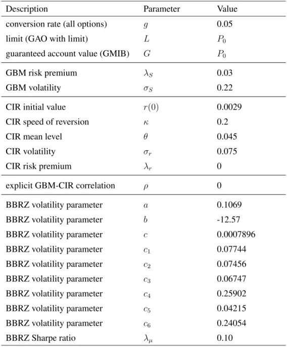
In our numerical analyses, we perform Monte Carlo simulations with 10,000 paths and 100 discretiza-tion steps per year. For simulating the forward force of mortality, we follow an approach proposed by Börger (2010, p. 254) using 150 standard normally distributed random variables in each path. We assume a 50-year-old male insured with a deferment period of 15 years and assume that the insurer uses the expected risk-neutral survival probabilities (hence implicitly including safety margins) as implied by the stochastic mortality model for hedging and pricing. The limiting age is set toω = 121.

All other parameters for the base case are given in Table 2, where the parameters for the GBM and the CIR model are taken from Graf et al. (2012)1 and the parameters for the BBRZ model are taken from Börger (2010).

Description Parameter Value

conversion rate (all options) g 0.05

limit (GAO with limit) L P0

guaranteed account value (GMIB) G P0

GBM risk premium λS 0.03

GBM volatility σS 0.22

CIR initial value r(0) 0.0029

CIR speed of reversion κ 0.2

CIR mean level θ 0.045

CIR volatility σr 0.075

CIR risk premium λr 0

explicit GBM-CIR correlation ρ 0

BBRZ volatility parameter a 0.1069 BBRZ volatility parameter b -12.57 BBRZ volatility parameter c 0.0007896 BBRZ volatility parameter c1 0.07744 BBRZ volatility parameter c2 0.07456 BBRZ volatility parameter c3 0.06747 BBRZ volatility parameter c4 0.25902 BBRZ volatility parameter c5 0.04215 BBRZ volatility parameter c6 0.24054 BBRZ Sharpe ratio λµ 0.10

Table 2: Input parameters for the base case.

1_{Only the initial short rate}_r

0 is adapted to current conditions and determined as the money market rate for overnight

(16)

4.2.1 Base case

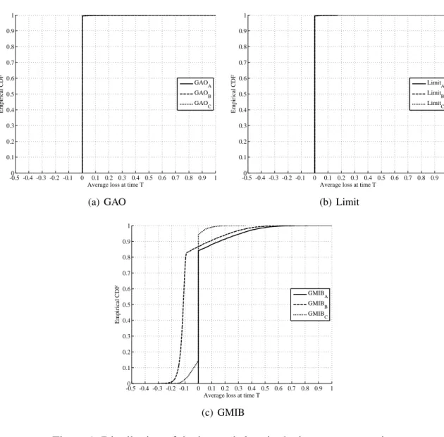
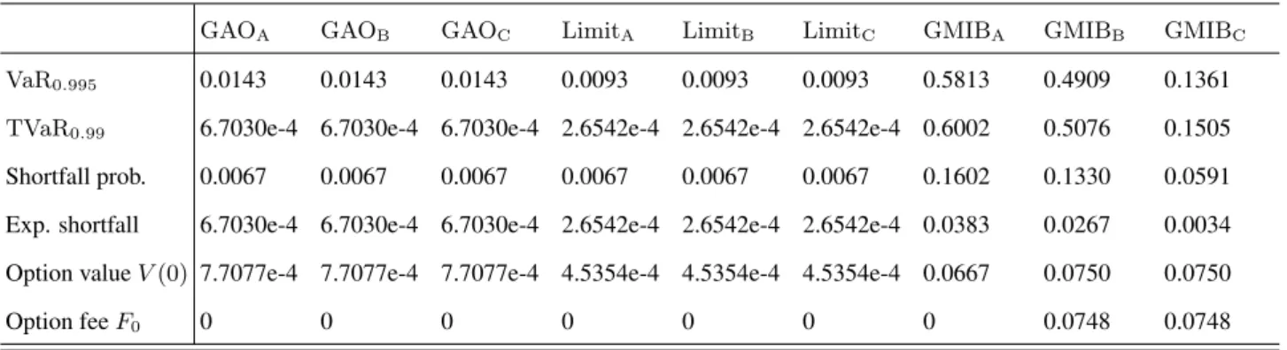
We start our numerical analyses by displaying in Figure 1 the distribution of the insurer’s loss at ma-turityT for all three considered annuity conversion options and all three considered risk management strategies in the given base case scenario. The respective risk measures are shown in Table 3. All values are given relative to the single premium paid.

-0.5 -0.4 -0.3 -0.2 -0.10 0 0.1 0.2 0.3 0.4 0.5 0.6 0.7 0.8 0.9 1 0.1 0.2 0.3 0.4 0.5 0.6 0.7 0.8 0.9 1

Average loss at time T

E m p ir ic al C D F GAO A GAO B GAO C (a) GAO -0.5 -0.4 -0.3 -0.2 -0.10 0 0.1 0.2 0.3 0.4 0.5 0.6 0.7 0.8 0.9 1 0.1 0.2 0.3 0.4 0.5 0.6 0.7 0.8 0.9 1

E m p ir ic al C D F Limit A Limit B Limit C (b) Limit -0.5 -0.4 -0.3 -0.2 -0.10 0 0.1 0.2 0.3 0.4 0.5 0.6 0.7 0.8 0.9 1 0.1 0.2 0.3 0.4 0.5 0.6 0.7 0.8 0.9 1

E m p ir ic al C D F GMIB A GMIB_B GMIB C (c) GMIB

Figure 1: Distribution of the insurer’s loss in the base case scenario.

In the base case scenario, where the long term interest rate level θ = 0.045 is relatively high compared to a rather low guaranteed conversion rate g = 0.05, the option fee F0 charged under

strategy B and C is equal to zero in the case of GAOs (with and without limit).2 As a result, all considered risk management strategies for GAO and Limit, respectively, show the same distribution and the insurer never faces any profit (negative loss) from these options. Nevertheless, there is a slightly positive option valueV(0) and a slightly positive probability of almost 1% that the GAO is in the money at maturity T. If it is in the money, it is in the money for the GAO version as well as for the Limit version of the product. It is only the extent of the insurer’s loss that might be different

2_{Remember that we assume that the insurer does not use stochastic mortality when calculating the option fee}_F

0and

(17)

GAOA GAOB GAOC LimitA LimitB LimitC GMIBA GMIBB GMIBC

VaR0.995 0.0143 0.0143 0.0143 0.0093 0.0093 0.0093 0.5813 0.4909 0.1361

TVaR0.99 6.7030e-4 6.7030e-4 6.7030e-4 2.6542e-4 2.6542e-4 2.6542e-4 0.6002 0.5076 0.1505

Shortfall prob. 0.0067 0.0067 0.0067 0.0067 0.0067 0.0067 0.1602 0.1330 0.0591 Exp. shortfall 6.7030e-4 6.7030e-4 6.7030e-4 2.6542e-4 2.6542e-4 2.6542e-4 0.0383 0.0267 0.0034 Option valueV(0) 7.7077e-4 7.7077e-4 7.7077e-4 4.5354e-4 4.5354e-4 4.5354e-4 0.0667 0.0750 0.0750

Option feeF0 0 0 0 0 0 0 0 0.0748 0.0748

Table 3: Selected risk measures of the insurer’s loss in the base case scenario.

for GAO and Limit. However, due to the rather low probability that the option is in the money at all, the risk of these guarantees seems negligible. Even in the 99.5th percentile, the loss of the insurer is below 1.5% of the single premium.

The GMIB guarantee shows a completely different risk profile. Under strategy A, where the insurer neither charges an option fee nor hedges its financial risk, the insurer never makes a profit (negative loss) but faces a loss in 16% of the cases. While the GAO needs sufficiently low interest rates and low mortality rates to be in the money, the GMIB guarantee can also be triggered by low fund values. Thus, most of the scenarios where the insurance company faces a loss are scenarios of falling fund prices, mostly combined with rather low interest rates and low mortality probabilities.

Under the strategies B and C, the insurer charges for the GMIB guarantee an option fee of F0 =

7.48%of the single premium paid. The corresponding option value isV(0) = 7.50%.

Under strategy B, where the insurer just charges this option fee but does not buy any hedging instruments, there is a high probability for the insurer to make a small profit. This profit comes from the option fee and the interest rate earned on it in all cases where the guarantee is not or only slightly in the money at maturity. However, if the guarantee is in the money, it is very unlikely that the option fee is enough to cover the liability. The shortfall probability in this case equals 13.3% while the expected shortfall amounts to almost 3% of the single premium paid. Losses can reach an amount of up to 50% of the single premium paid in the 99.5% VaR or 99% TVaR in case no hedging is in place. This clearly shows that, if the risk based capital is calculated under market consistent valuation approaches such as Solvency II or Swiss Solvency Test, such a strategy would hardly reduce the capital requirements. Under strategy C, the insurer uses the option fee to purchase interest rate and equity hedges ac-cording to its prudent mortality assumptions. There are a number of cases where neither the hedge instruments bought nor the claim the insurer has to pay have any positive value at maturityT. These cases lead to an insurer’s loss of zero. There is a probability of almost 15% that the value of the hedge instruments is greater than the value of the insured’s claim at maturityT. In most of these cases, no claim is to be paid at all but the hedge instruments have some positive payoff. All these cases lead to some profit for the insurer. In the opposite event where the hedge instruments are not sufficient to cover the insurance claims, the insurer faces a loss. This happens in roughly 6% of the cases with an expected shortfall of 0.3%. Compared to strategy B, 99.5% VaR and 99% TVaR can be significantly reduced by the capital market hedge from roughly 50% to 13% - 15%. However, the remaining risk resulting from stochastic mortality still leads to rather high capital requirements.

The results in this base case scenario, where long term interest rate assumptions are rather high compared to guaranteed conversion rates, show that the GMIB guarantee seems to carry a much higher risk for the insurer than GAOs. The main reason for this result, however, is the rather high

(18)

interest rate level and the fact that the GAO is far out of the money at inception of the contract. This can be seen by the following sensitivity analyses with lower interest rate levels.

4.2.2 Sensitivity with respect to the level of interest rates

In this section, we provide some sensitivity analyses for lower long term interest rate assumptions. We distinguish between an environment of ‘low interest rates’ (θ = 0.03) and an environment of ‘very low interest rates’ (θ= 0.015). All other parameters remain unchanged.

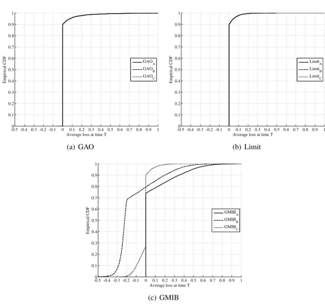
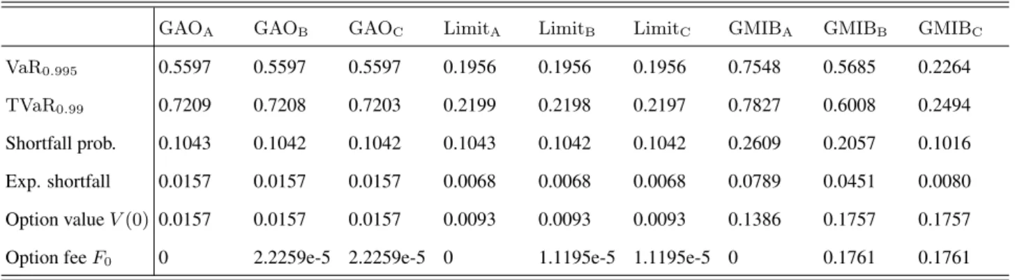
Figure 2 shows the distribution of the insurer’s standardized loss at maturityT for all three consid-ered annuity conversion options and all three considconsid-ered risk management strategies in the scenario of low interest rates. The respective risk measures are shown in Table 4.

-0.5 -0.4 -0.3 -0.2 -0.10 0 0.1 0.2 0.3 0.4 0.5 0.6 0.7 0.8 0.9 1 0.1 0.2 0.3 0.4 0.5 0.6 0.7 0.8 0.9 1

E m p ir ic al C D F GAO A GAO B GAO_C (a) GAO -0.5 -0.4 -0.3 -0.2 -0.10 0 0.1 0.2 0.3 0.4 0.5 0.6 0.7 0.8 0.9 1 0.1 0.2 0.3 0.4 0.5 0.6 0.7 0.8 0.9 1

E m p ir ic al C D F Limit A Limit B Limit_C (b) Limit -0.5 -0.4 -0.3 -0.2 -0.10 0 0.1 0.2 0.3 0.4 0.5 0.6 0.7 0.8 0.9 1 0.1 0.2 0.3 0.4 0.5 0.6 0.7 0.8 0.9 1

E m p ir ic al C D F GMIB_A GMIB B GMIB_C (c) GMIB

Figure 2: Distribution of the insurer’s loss in a scenario of low interest rates.

The first and very obvious result is that in comparison to the base case scenario, all considered annuity conversion options become more valuable from a client’s perspective and riskier from an insurer’s perspective.

However, the option fee for the GAO charged under the strategies B and C is still practically zero. More precisely, assuming deterministic mortality tables as described in Section 3.3, the insurer cal-culates a slightly positive option fee that is below 0.01% of the single premium. Thus again, for the

(19)

GAOA GAOB GAOC LimitA LimitB LimitC GMIBA GMIBB GMIBC VaR0.995 0.5597 0.5597 0.5597 0.1956 0.1956 0.1956 0.7548 0.5685 0.2264 TVaR0.99 0.7209 0.7208 0.7203 0.2199 0.2198 0.2197 0.7827 0.6008 0.2494 Shortfall prob. 0.1043 0.1042 0.1042 0.1043 0.1042 0.1042 0.2609 0.2057 0.1016 Exp. shortfall 0.0157 0.0157 0.0157 0.0068 0.0068 0.0068 0.0789 0.0451 0.0080 Option valueV(0) 0.0157 0.0157 0.0157 0.0093 0.0093 0.0093 0.1386 0.1757 0.1757

Option feeF0 0 2.2259e-5 2.2259e-5 0 1.1195e-5 1.1195e-5 0 0.1761 0.1761

Table 4: Selected risk measures of the insurer’s loss in a scenario of low interest rates.

GAO and the Limit guarantee, there is practically no difference between the considered risk manage-ment strategies. The option value taking into account stochastic mortality, however, already amounts to 1.57% of the single premium in the GAO case and 0.93% of the single premium in the case of the limited GAO. This shows the effect of the pricing methodology commonly used in practice, which systematically ignores one source of risk, namely stochastic mortality.

Under the assumptions of low interest rates, the difference between the GAO and the limited GAO becomes visible, especially when the tail risk is considered. While for an unlimited GAO, the 99.5% VaR (99% TVaR resp.) reaches a level of 56% (72% resp.), the limited GAO only faces a risk of 20% (22% resp.) of the single premium. Note that the shortfall probability is still the same (10%) for both options since the shortfall is triggered by the same scenarios, namely when low interest rates coincide with low mortality rates. However, in a scenario of high fund returns the extent of the shortfall is higher if no limit is set on the GAO. This can also be seen by comparing the expected shortfall of 1.57% in the GAO case and 0.68% in the Limit case.

Under low interest rates, the GMIB generally shows a similar pattern as in the base case scenario. Naturally, guarantees become more valuable compared to the base case scenario and thus risk be-comes more pronounced. In the case where no option fee is charged, the shortfall probability in-creases to 26%, the expected shortfall inin-creases to 8% and the tail risk inin-creases to 75% - 78% of the single premium paid. If the option fee of 17.61% is charged but no appropriate hedging is in place, the risk is reduced but still high.

Even if hedging is in place, that is, the insurer follows strategy C, the risk increases compared to the base case parameter setting. However, comparing the GAO and the GMIB guarantee in more detail, there are some effects that deserve a little more attention. If guarantees are not adequately hedged, the GMIB is much riskier than the GAO. It shows a much higher option value as well as higher shortfall probabilities and expected shortfalls. However, the tail risk is similar for both products. If the insurance company hedges capital market risks, the risk of the GMIB can be heavily reduced while practically no hedging effect can be seen for the GAO products. The latter effect is rather clear since the option fees for the GAO products are practically zero. For the GMIB, however, the rather high option fee is used to buy a hedge portfolio according to the expected probabilities of surviving. Still, losses occur due to deterministic mortality assumptions. The shortfall probability reaches a similar level in the hedged GMIB as in the hedged GAO case (roughly 10%). The potential loss, however, is limited in the GMIB case while it is unlimited in the GAO case. Furthermore, as described above, for the insurer the considered hedging strategy works better for the GMIB than for the considered GAO product. This leads to a situation where, even though the shortfall probabilities are similar for all product designs, the expected shortfall as well as the tail risk is much higher in the GAO case when

(20)

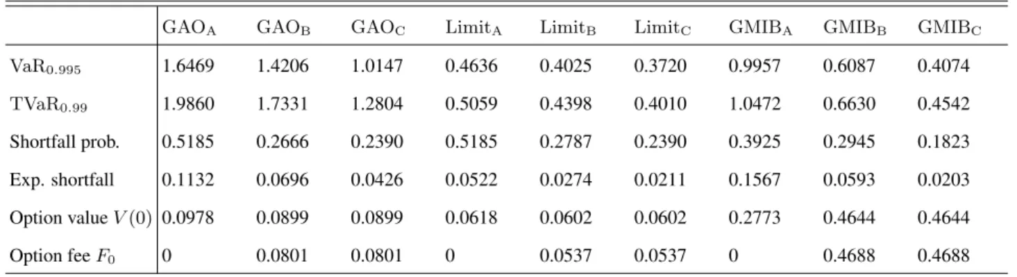
compared to the GMIB case. The hedged GMIB even shows a similar tail risk as the limited GAO. The effects are even more pronounced in a scenario of very low interest rates (θ= 0.015). Figure 3 shows the corresponding distribution of the insurer’s standardized loss at maturity T for all three considered annuity conversion options and all three considered risk management strategies. The respective risk measures are shown in Table 5.

-0.5 -0.4 -0.3 -0.2 -0.10 0 0.1 0.2 0.3 0.4 0.5 0.6 0.7 0.8 0.9 1 0.1 0.2 0.3 0.4 0.5 0.6 0.7 0.8 0.9 1

E m p ir ic al C D F GAO_A GAO B GAO_C (a) GAO -0.5 -0.4 -0.3 -0.2 -0.10 0 0.1 0.2 0.3 0.4 0.5 0.6 0.7 0.8 0.9 1 0.1 0.2 0.3 0.4 0.5 0.6 0.7 0.8 0.9 1

E m p ir ic al C D F Limit_A Limit B Limit_C (b) Limit -0.5 -0.4 -0.3 -0.2 -0.10 0 0.1 0.2 0.3 0.4 0.5 0.6 0.7 0.8 0.9 1 0.1 0.2 0.3 0.4 0.5 0.6 0.7 0.8 0.9 1

E m p ir ic al C D F GMIB A GMIB B GMIB C (c) GMIB

Figure 3: Distribution of the insurer’s loss in a scenario of very low interest rates.

In an environment of very low interest rates, again, all guarantees become more valuable from a client’s perspective and all products become riskier from an insurer’s perspective. The effect, though, is much more pronounced for the GAO product design than for the GMIB product design. Under very low interest rates, the GAO product shows by far the highest risk, even if the considered hedging strategy is in place. The tail risk in the 99.5% VaR and 99% TVaR, even after hedging, exceeds the single premium. Although – in contrast to the scenario of low interest rates – the option fee charged is positive, the considered risk management strategy C hardly reduces the risk. This is because the question whether or not the option is in the money heavily depends on the development of mortality which is not hedged due to the lack of mortality hedge instruments. In contrast, for the GMIB option, the question whether the option is in the money primarily depends on the development of the fund which is hedged. Hence, although the GMIB hedge is also not perfect, the hedge at least returns some

(21)

GAOA GAOB GAOC LimitA LimitB LimitC GMIBA GMIBB GMIBC VaR0.995 1.6469 1.4206 1.0147 0.4636 0.4025 0.3720 0.9957 0.6087 0.4074 TVaR0.99 1.9860 1.7331 1.2804 0.5059 0.4398 0.4010 1.0472 0.6630 0.4542 Shortfall prob. 0.5185 0.2666 0.2390 0.5185 0.2787 0.2390 0.3925 0.2945 0.1823 Exp. shortfall 0.1132 0.0696 0.0426 0.0522 0.0274 0.0211 0.1567 0.0593 0.0203 Option valueV(0) 0.0978 0.0899 0.0899 0.0618 0.0602 0.0602 0.2773 0.4644 0.4644 Option feeF0 0 0.0801 0.0801 0 0.0537 0.0537 0 0.4688 0.4688

Table 5: Selected risk measures of the insurer’s loss in a scenario of very low interest rates.

positive payoff in most scenarios where the option’s payoff is positive. This is not the case for the GAO options.

These sensitivities certainly show that guarantees that have been sold in times of very high interest rates with seemingly no value and almost no risk, now turn out to be extremely valuable and risky. 4.2.3 Sensitivity with respect to equity volatility

As a next step, we focus on the impact of different equity volatility assumptions on the risk of the different product designs. Since under the base case assumptions the GAO did not show any risk at all, we perform the sensitivity analysis with respect to equity volatility under the scenario of low interest rates. Thus, throughout this section we assume a long term interest rate level of θ = 0.03. We start with the case of low volatilities by assumingσS = 0.1as opposed to the base case where

σS = 0.22and also show the case of high volatilities by assumingσS = 0.3.

Figure 4, respectively 5, shows the distribution of the insurer’s standardized loss at maturityT for all three considered annuity conversion options and all three considered strategies in the scenario of low, respectively high, equity volatility. The corresponding risk measures are shown in Table 6, respectively 7.

First, we want to mention that the shortfall probability of all GAO product designs is not affected by equity volatility. The question whether a GAO product is in the money or not is only triggered by interest rates and mortality rates. Equity (and thus equity volatility) only has an impact on the extent of the insurer’s loss if the option is in the money. Since the insurer’s loss increases in the fund value for the unlimited GAO, the risk is increasing in equity volatility. The higher the volatility, the higher is the likelihood of high fund values when the GAO is triggered. The 99.5% VaR (99% TVaR resp.) is given by 48% (55% resp.) in the case of low equity volatilities and 61% (87% resp.) in the case of high equity volatilities compared to 56% (72% resp.) before. Thus, the GAO shows a rather low sensitivity to changing equity volatility, in particular compared to the previously shown sensitivity with respect to interest rates. Apparently, the product’s exposure to interest rates and mortality seems to be higher than its exposure to changing equity volatility. This is even further pronounced in the case of the limited GAO which is hardly affected by changing volatilities since the limit completely absorbs the increased risk.

The GMIB shows a different sensitivity to equity volatility than the GAOs. Remember that the GMIB guarantee is not only triggered by low interest rates combined with low mortality rates, but also by low fund values. Thus, high equity volatility leads to a high risk for the insurer and this risk can be seen in any of the risk measures. The shortfall probabilities rise from 2.4% in the unhedged case (1.4% in the hedged case resp.) to 42% (15% resp.) if the volatility is increased fromσS = 0.1to

(22)

-0.5 -0.4 -0.3 -0.2 -0.10 0 0.1 0.2 0.3 0.4 0.5 0.6 0.7 0.8 0.9 1 0.1 0.2 0.3 0.4 0.5 0.6 0.7 0.8 0.9 1

Figure 4: Distribution of the insurer’s loss in a scenario of low equity volatility and low interest rates.

VaR0.995 0.4844 0.04843 0.4844 0.2157 0.2157 0.2157 0.2158 0.1966 0.0873

TVaR0.99 0.5490 0.5490 0.5486 0.2423 0.2423 0.2422 0.2474 0.2286 0.1114

Shortfall prob. 0.1043 0.1042 0.1042 0.1043 0.1042 0.1042 0.0241 0.0231 0.0141 Exp. shortfall 0.0160 0.0160 0.0160 0.0077 0.0077 0.0077 0.0033 0.0029 0.0012 Option valueV(0) 0.0160 0.0160 0.0160 0.0114 0.0114 0.0114 0.0321 0.0367 0.0367

Option feeF0 0 1.9435e-5 1.9435e-5 0 1.3947e-5 1.3947e-5 0 0.0346 0.0346

Table 6: Selected risk measures of the insurer’s loss in a scenario of low equity volatility and low interest rates.

(23)

-0.5 -0.4 -0.3 -0.2 -0.10 0 0.1 0.2 0.3 0.4 0.5 0.6 0.7 0.8 0.9 1 0.1 0.2 0.3 0.4 0.5 0.6 0.7 0.8 0.9 1

Figure 5: Distribution of the insurer’s loss in a scenario of high equity volatility and low interest rates.

VaR0.995 0.6126 0.6125 0.6126 0.1851 0.1850 0.1851 0.9116 0.5954 0.2534

TVaR0.99 0.8744 0.8743 0.8736 0.2028 0.2028 0.2026 0.9395 0.6295 0.2813

Shortfall prob. 0.1043 0.1042 0.1042 0.1043 0.1042 0.1042 0.4178 0.3170 0.1483 Exp. shortfall 0.0156 0.0156 0.0156 0.0058 0.0058 0.0058 0.1706 0.0726 0.0117 Option valueV(0) 0.0152 0.0152 0.0152 0.0078 0.0078 0.0078 0.2164 0.2716 0.2716

Option feeF0 0 2.5701e-5 2.5701e-5 0 9.3583e-6 9.3583e-6 0 0.2729 0.2729

Table 7: Selected risk measures of the insurer’s loss in a scenario of high equity volatility and low interest rates.

(24)

σS = 0.3. The expected shortfalls even increase from 0.3% in the unhedged case (0.1% in the hedged

case resp.) to 17.1% (1.17% resp.). A similar pattern, though on a different scale, can be seen when comparing tail risk measures such as VaR and TVaR. Under any considered risk measure, the impact of volatility is much higher in the unhedged case than in the hedged case.

Overall, the GMIB product shows a much higher sensitivity to equity volatility than the GAOs. For lower equity volatility, the risk of the GMIB product is significantly reduced while the effect on the GAOs is less pronounced. In the case of high equity volatility, the GMIB and the unlimited GAO show very high tail risks that can only be partly reduced by hedging in the GMIB product design and hardly reduced by hedging in the GAO product design.

4.2.4 Sensitivity with respect to the volatility of mortality

Finally, we analyze the impact of the volatility of mortality on the risk of the different product de-signs. As in previous sections, we provide this sensitivity under the scenario of low interest rates. Thus, throughout the section we assume a long term interest rate level of θ = 0.03. Note that the BBRZ model uses a variety of different (volatility) parameters. As a sensitivity for high volatility of mortality, in this section, we double the general level of volatilityσ1 (cf. Appendix A) and thus use

c1 = 0.15488as opposed toc1 = 0.07744in the base case.

Figure 6 shows the distribution of the insurer’s standardized loss at maturityT for all three consid-ered annuity conversion options and all three considconsid-ered risk management strategies in the scenario of high volatility of mortality. The corresponding risk measures are shown in Table 8.

First we want to study the impact on the insurer’s pricing, i.e. on the option feeF0. Since for pricing

the insurer uses deterministic mortality tables given by the expected risk-neutral survival probabilities (including safety margins) as implied by the stochastic mortality model, the sensitivity shown here also changes the deterministic table used by the insurer and thus the option feeF0. While previously

the option fee for the GAO product designs was practically 0, now the option fee becomes slightly positive. However, it is still below 1% of the single premium paid for both GAO option types. The option value, however, increases to over 3% in the GAO case and to almost 2% for the limited GAO. At the same time, there is only little impact of an increased volatility of mortality on the price and the value of the GMIB option.

A look at the different risk measures reveals a similar picture. The GMIB option shows much less sensitivity to a change in the volatility of mortality than the GAO. Of course, all risk measures also increase for the GMIB, but the impact is relatively low. The reason for this is mainly given by the fact that for a GMIB option, adverse developments of mortality (i.e. low mortalities) can be compensated by a good stock market performance.

For the GAO, the risk significantly increases with increasing volatility of mortatlity. The 99.5% VaR (99% TVaR resp.) is given by 108% (137% resp.) of the single premium paid in the case of high volatility of mortality compared to 56% (72% resp.) in the case of the previous volatility of mortality. These numbers can only be slightly reduced to 99% (128%) if hedging is in place. Thus, the company’s risk almost doubles if the general level of the volatility of mortality is twice as high. A similar effect (though lower in absolute numbers) can be observed for the limited GAO. This shows that the sensitivity to changing mortality is higher for the GAO product design compared to the GMIB product.

We finally want to mention that we have calculated further sensitivities with respect to the volatility of mortality as well as with respect to other capital market parameters, including the equity risk premium and the correlation between equity and interest rates. Since the additional analyses did not reveal any structurally different results, we refrain from showing further sensitivities.

(25)

-0.5 -0.4 -0.3 -0.2 -0.10 0 0.1 0.2 0.3 0.4 0.5 0.6 0.7 0.8 0.9 1 0.1 0.2 0.3 0.4 0.5 0.6 0.7 0.8 0.9 1

E m p ir ic al C D F GAO A GAO_B GAO C (a) GAO -0.4 -0.3 -0.2 -0.1 0 0.1 0.2 0.3 0.4 0.5 0.6 0.7 0.8 0.9 1 0 0.1 0.2 0.3 0.4 0.5 0.6 0.7 0.8 0.9 1

E m p ir ic al C D F Limit A Limit_B Limit C (b) Limit -0.5 -0.4 -0.3 -0.2 -0.10 0 0.1 0.2 0.3 0.4 0.5 0.6 0.7 0.8 0.9 1 0.1 0.2 0.3 0.4 0.5 0.6 0.7 0.8 0.9 1

E m p ir ic al C D F GMIB A GMIB_B GMIB C (c) GMIB

Figure 6: Distribution of the insurer’s loss in a scenario of high volatility of mortality and low interest rates.

VaR0.995 1.0893 1.0659 0.9870 0.3404 0.3330 0.3221 0.8023 0.6040 0.3068 TVaR0.99 1.3724 1.3471 1.2767 0.3514 0.3438 0.3318 0.8514 0.6453 0.3290 Shortfall prob. 0.1608 0.1448 0.1395 0.1608 0.1472 0.1395 0.2649 0.2016 0.0862 Exp. shortfall 0.0369 0.0347 0.0318 0.0151 0.0140 0.0130 0.0833 0.0439 0.0095 Option valueV(0) 0.0322 0.0319 0.0319 0.0187 0.0187 0.0187 0.1483 0.1952 0.1952 Option feeF0 0 0.0092 0.0092 0 0.0055 0.0055 0 0.2088 0.2088

Table 8: Selected risk measures of the insurer’s loss in a scenario of high volatility of mortality and low interest rates.

(26)

5 Conclusion

The present paper provides a framework for a joint analysis of financial and longevity guarantees and applies this framework to different annuity conversion options in deferred unit-linked annuities. We analyzed and compared two versions of so-called guaranteed annuity options as well as guaranteed minimum income benefits with respect to the value of the option and the resulting risk for the in-surer. Besides the different option types, we considered different risk management strategies of the insurance company dealing with these options. Since the payoff of the options (and hence also their value and the resulting risk) depends on the development of the underlying fund, interest rates, and mortality, we used a combined stochastic model for our analyses where both, the financial market as well as future survival probabilities, are modeled stochastically.

Although all options depend on all considered risk drivers (fund value, interest rates and mortality), there are structural differences between the options. First, the risk of decreasing fund values turns out to be the predominant risk in GMIBs. At the same time it is also the main driver for the question whether or not the option is in the money. In contrast, for traditional as well as limited GAOs, interest and mortality risks are of higher relevance since they trigger whether or not the option is in the money. Only the extent of the insurer’s loss (in case the option is in the money) increases with increasing fund value. The second structural difference is that for the GMIBs, the payoff of the option is negatively correlated with the fund value whereas it is positively correlated for the GAOs.

Our results show that the different annuity conversion options can have significantly different option values and that different risk management strategies can lead to a significantly different risk for the insurance company. More precisely, we find that in our base case scenario, where long term market rate assumptions are rather high compared to the guaranteed conversion rate, a GMIB guarantee constitutes a much higher risk for the insurer than GAOs. The main reason for this result, however, is that due to the rather high interest rate level, the GAO is already far out of the money at inception of the contract. Reducing the level of the long term interest rate assumption yields a much higher option value and also a higher risk for the insurer for all considered annuity conversion options. However, under low interest rate assumptions, the risk is the highest for the GAO. Even though under the real world measure the insurer’s shortfall probability might be comparable to other product designs, the potential extent of the loss is the highest for GAOs. Still, the GAO’s risk-neutral option value remains much lower than the GMIB’s option value which can be observed throughout all our analyses. This “change of measure effect” results from the equity risk premium and is particularly pronounced since the payoff of the GMIB option increases with decreasing fund value whilst the payoff of the GAO decreases.

Comparing different risk management strategies shows that, as expected, charging a fee and in-vesting it in the bank account only slightly reduces the insurer’s loss compared to charging no fee, since the charged fee is low compared to potential losses in the tail of the loss distribution. In con-trast, investing the fee in suitable hedging instruments is much more effective, especially for GMIBs. The loss distribution for GMIBs significantly changes to the insurer’s advantage if financial risks are hedged. Hedging is more efficient in the GMIB case than in the GAO case because here, the main driver for the question whether the option is in the money, namely the fund value, can be hedged. Hence, although the hedge is not perfect due to the lack of mortality hedge instruments, the hedge has a positive payoff in at least most of the scenarios where the GMIB is in the money. This is in sharp contrast to the GAO options, where the question whether the option is in the money heavily depends on the mortality development which is not hedged under our strategies.

Furthermore, the GMIB product displays a much higher sensitivity with respect to equity volatility than the GAO. In the case of high equity volatility, all products show very high tail risks that can