University of Alberta

(1)

University of Alberta

Dynamic Behavior of Surface-bonded Piezoelectric Sensor with Interfacial Debonding

by Hongbo Huang

A thesis submitted to the Faculty of Graduate Studies and Research in partial fulfillment of the requirements for the degree of

Master of Science

Department of Mechanical Engineering

©Hongbo Huang Fall 2009 Edmonton, Alberta

Permission is hereby granted to the University of Alberta Libraries to reproduce single copies of this thesis and to lend or sell such copies for private, scholarly or scientific research purposes only. Where the thesis is converted to, or otherwise made available in digital form, the University of Alberta will advise potential users

of the thesis of these terms.

The author reserves all other publication and other rights in association with the copyright in the thesis and, except as herein before provided, neither the thesis nor any substantial portion thereof may be printed or

(2)

Examining Committee

Xiaodong Wang, Mechanical Engineering

Zihui Xia, Mechanical Engineering

(3)

ABSTRACT

The performance of smart structures depends on the dynamic electromechanical behavior of piezoelectric sensors/actuators and the bonding condition along the interface. This thesis contents a theoretical study of the coupled electromechanical characteristics of a surface-bonded piezoelectric sensor with interfacial debonding, which is subjected to high frequency mechanical loads. A one dimensional sensor model is proposed. Analytical solutions based on the integral equation method are provided.

Numerical simulation is conducted to evaluate the effects of different parameters upon the dynamic load transfer between the sensor and the host medium. The results indicate that, the material combination, the sensor geometry, and the loading frequency, affect the load transfer significantly. The analytical solution of the elastic wave field in the host medium is obtained and used to evaluate the effects of different parameters upon the resulting wave field. The theoretical solution demonstrates the basic properties of wave propagation under current loading conditions.

(4)

ACKNOWLEDGEMENTS

I would like to express my deepest gratitude to Dr. Xiaodong Wang, my supervisor, for his constant encouragement and guidance. His trust, support and invaluable advice made every stage of my research work go smoothly and pleasantly. My grateful sentiments come from the bottom of my heart.

Secondly, my thanks would go to my parents and my husband. Their support, understanding and endless love are the source of my courage and strength to conquer any difficulty in my study and life.

Finally but not least, I would like to thank all my friends, who share their time with me, listen to me, and help me out during tough periods.

(5)

List of Figures

3.1: The geometry of the sensor system ... 14

3.2: The stress field of the sensor system ... 14

3.3: The stress field inside the sensor ... 16

3.4: The stress field inside the host medium ... 19

3.5: UAmplitude of * s y ε ... 27

3.6: Amplitude of κ with different loading frequencies ... 30

3.7: Phase angle of κ under different loading frequencies ... 30

3.8: Amplitude of κ with different material combinations ... 31

3.9: Phase angle of κ with different material combinations ... 31

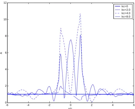
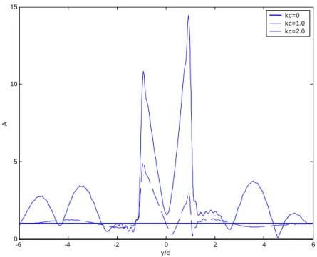
3.10: Amplitude of κ( y)_{with relatively low kc (q = 0.5,}

υ

=5.0) ... 34

3.11: Amplitude of κ( y)_{with relatively high kc (q = 0.5,}

υ

=5.0) ... 34

3.12: Amplitude of κ( y)_{with different kc (q = 5.0,}

υ

=5.0) ... 35

3.13: Amplitude of κ( y)_{under different kc (q = 0.5,}

υ

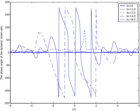
=20.0) ... 35

3.14: Phase angle of κ( y)_{under different kc (q = 0.5,}

υ

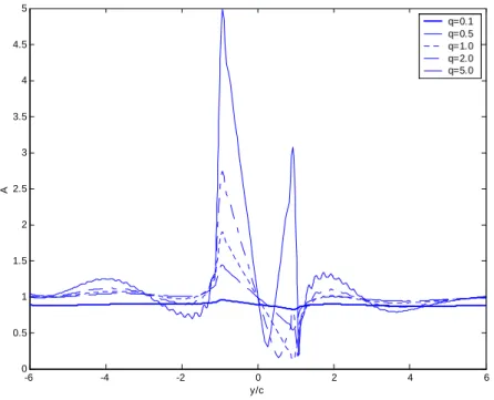
=20.0) ... 36

3.15: Amplitude of κ(y)with different q (kc = 1,

υ

=5.0UU) ... 38

3.16: Amplitude of κ( y) with different q (kc = 4, υ =5.0UU) ... 38

3.17: Amplitude of κ( y)with different geometries (kc = 1.0, q = 0.5) ... 41

3.18: The distribution of V (_{kc = 2.0, q = 0.5,}

υ

=20.0) ... 41

3.19: Amplitude of Vmax under different loading frequencies (q = 0.5) ... 42

3.20: Amplitude of Vmax under different loading frequencies (q = 5.0) ... 42

4.1: The integration path in complex s plane ... 42

4.2: The amplitude of * y σ (kc = 3.0, q = 0.5,

υ

=20.0) ... 54 4.3: The amplitude of d* y σ (kc = 3.0, q = 0.5,

υ

=20.0) ... 55 4.4: The amplitude of * yz τ (kc = 3.0, q = 0.5,

υ

=20.0) ... 55 4.5: The amplitude of σ*z (kc = 3.0, q = 0.5,

υ

=20.0) ... 56

(8)

4.6: The amplitude of σdz* (kc = 3.0, q = 0.5,

υ

=20.0) ... 56

4.7: The amplitude of τdyz0*(

υ

=20.0) ... 57

4.8: The comparison of the far field stress σzf* ... 64

4.9: The far field stress f* z

σ (kc = 1.0) ... 65 4.10: The far field stress f*

z

σ (kc = 2.0) ... 65 4.11: The far field stress σzf* (kc = 4.0) ... 66

(9)

List of Symbols

c Half length of the interfacial debonding h The thickness of the sensor

x, y, z Carstesian coordinates

ω

Circular frequency of the incident wave

0

θ

Incident angle of the incident wave to the vertical line

T

L k

k , Longitudinal wave number, transverse wave number

0

k Apparent wave number of the incident wave

s

k Apparent wave number of the incident wave in the sensor

T

L c

c , Longitudinal wave speed, transverse wave speed

0

c Surface wave speed

0

A Amplitude of surface wave ψ Phase angleof surface wave

∇ Laplacian operator

Ψ

Φ, Displacement potential functions

s Transform variable of Fourier transform i Squar root of -1 t Time ij uv Displacement vector ij u Magnitude of displacement ij

ε Magnitude of strain components

0 ij

u Magnitude of the displacement of the incident wave

I ij

u Magnitude of the displacement field in the host medium with free surface

I ij

ε Magnitude of the strain field in the host medium with free surface

I

A Amplitude of u ijI s

ij

(10)

h ij

u Magnitude of the displacement field in the host medium

τ

ij

u Magnitude of the dynamic displacement field in the host medium by

τ

s ij

ε Magnitude of the strain components in the sensor

* s ij

ε Magnitude of the normalized strain compoments in the sensor

ij

σv Stress tensor

ij

σ Magnitude of stress components

* ij

σ Magnitude of the normalized stress components

s ij

σ Magnitude of the stress induced by the sensor

d ij

σ Magnitude of the stress by interfacial debonding

f ij

σ Magnitude of far field stress in the host medium by interfacial debonding

0 ij

σ Magnitude of surface stress

0 d ij

σ Magnitude of surface stress contributed by interfacial debonding τ Magnitude of interfacial shear stress

Z

D Magnitude of electric displacement

Z

E Magnitude of electric field intensity

ij

c Elastic constants of piezoelectric material

ij

e Piezoelectric constants of piezoelectric material

i

λ Dielectric constants of piezoelectric material

h

E Young’s Modulus of the host medium

s

E The effective modulus of the sensor v Poisson’s ratio of the host medium µ The shear modulus of the host medium

h

s ρ

ρ , Mass density of the sensor, the host medium q Material combination factor

(11)

j

j U

T , Chebyshev polynomials of the first and the second kind

j

C Coefficients of the Chebyshev polynomials ϕ Dislocation density function

κ

Dynamic strain ratio for imperfect bonding case )

( y

κ

Dynamic strain ratio for imperfect bonding case V Voltage distribution along the sensor

max

V Maximum value of the magnitude of the voltage along the sensor V Normalized voltage distribution along the sensor

max

(12)

§1 Introduction

1.1 Background

Structural Health Monitoring (SHM) is a methodology in the interdisciplinary engineering field devoted to the monitoring and assessment of structural health and durability, integrated with remote sensing, smart materials, and computer based knowledge systems to allow engineers observe the performance of the structures over time. For those large structures or special structures like aero vehicles or buried pipelines, it is impractical to perform in-service monitoring by high-in-cost traditional nondestructive testing/evaluation (NDT/NDE) techniques such as ultrasonic and eddy currents. Besides, recent incidents in the commercial aircraft industry have raised doubts over the reliability of NDT techniques to detect cracking and corrosion. While new technology generally improves sensitivity of detection techniques it is essential that they can be shown to have the appropriate detection reliability in actual use [1].

With the development of sensor systems, data acquisition, data communication and computational methodologies, instrumentation-based on-line monitoring by making use of sensors/actuators has been a widely accepted technology for in-situ monitoring and diagnosing structural health and conditions, replacing or combining with traditional nondestructive testing methods. Among the currently available options, piezoelectric sensors incarnate the superiority because they are low in cost, highly sensitive, compact/light weight, easily formed into different shapes or wired into sensor arrays. Because of the excellent dynamic response characteristics, piezoelectric SHM is widely used in elastic wave based testing, reading and analyzing the incipient information detected by surface-bonded or embedded-in piezoelectric sensors/actuators. Compared with traditional

(13)

in-service testing. Elastic wave based piezoelectric SHM can be performed in forms of either passive SHM or active SHM, while the former means a SHM system with only piezoelectric sensors which just “listen to” the structure health; and the latter means a SHM system with built-in actuators “interacting with” the structure by choosing suitable monitoring signals.

The efficiency of the monitoring is demonstrated by the coupled electromechanical dynamic behavior of the system, which is not only related by the sensor/actuator properties but also those of the host structure, as well as other parameters including loading frequencies and bonding conditions. A better understanding of the resulting wave propagation in the structure is also a prerequisite for achieving the goal of elastic wave based health monitoring. When the piezoelectric sensor/actuator is surface bonded to the host medium, high interfacial stress field may occur due to the material discontinuity [2]. The high stress concentration may lead to the reduction of the sensing/actuating ability of piezoelectric patches by undesired debonding especially in dynamic applications. Moreover, imperfect bonding between the patches and the host structure will change the phase and the amplitude of propagated waves significantly, as well as other important parameters used in monitoring techniques, resulting in false indications on the structural conditions without an efficient sensor-diagnostic process [3]. Therefore, more detailed analytical and experimental studies on the coupled dynamic behavior of surface-bonded piezoelectric layer(s) with interfacial debonding have to be performed, in order to evaluate the reliability and feasibility of surface-bonded sensor SHM systems.

Previous works have been done to study the complicated local stress field around the perfectly bonded sensor/actuators [4-8]. Recently, some researchers have studied the effects of bonding state on elastic wave generation and reception [9], as well as the dynamic behavior of the imperfectly surface-bonded sensor/actuator system [10-13].

(14)

1.2 Research Objectives

The objective of this thesis is to investigate the effects of the interfacial debonding upon the dynamic load transfer between a surface-bonded piezoelectric sensor and the elastic host medium, as well as the elastic wave propagation inside the host structure. A one dimensional sensor model will be established to simulate the coupled dynamic behavior of the system. Numerical simulation is conducted to study the effects of different loading frequencies, material combinations and sensor geometries on the dynamic electromechanical properties of the sensor under high frequency dynamic mechanical loads. The wave propagation generated by the surface-bonded sensor and the interfacial defection is studied by analytical method as well as numerical simulation.

1.3 Organization of the Thesis

The thesis is organized as follow. The current progress and relevant theories and techniques needed in modeling the sensor system are reviewed in Chapter 2. A one dimensional sensor model is established in Chapter 3, to evaluate the coupled dynamic behavior of the surface-bonded sensor system. Typical examples are provided to show the effects of the loading frequencies, material combinations and sensor geometries upon the load transfer and the sensor signals, and the results are compared between the perfect-bonding and imperfect-bonding conditions to investigate the influence of interfacial defection. In Chapter 4, the simulation of the elastic wave propagation generated by the sensor and the interfacial crack is conducted using the established one-dimension sensor model, to investigate the effects of the above parameters upon the resulting wave propagation. The basic properties of the generated wave are examined by the explicit forms near the interface and far field inside the host structure which can be analytically obtained. The last chapter, Chapter 5, summarizes the conclusions and contributions of the study and recommends some prospective topics for the

(15)

§2 Literature Review

2.1 History of Piezoelectricity and Piezoelectric Devices

Piezoelectricity phenomenon is firstly demonstrated experimentally by Pierre and Jacques Curie in the year of 1880 [14] which is the coupling between the material's mechanical and electrical behaviors. Simply speaking, electrical charges can be collected on its surface when the material is under mechanical stress. Conversely, when subjected to a voltage, a piezoelectric material will produce mechanical stress or deformation. In 1882, the core of piezoelectric applications science was established by the interactive work of European scientific community, which includes the identification of piezoelectric crystals on the basis of asymmetric crystal structure, the reversible exchange of electrical and mechanical energy, and the usefulness of thermodynamics in quantifying complex relationships among mechanical, thermal and electrical variables. The work is extended in the future 25 years and the first serious application of piezoelectric took place during World War I in 1917. P. Langevin and his French co-workers developed an ultrasonic submarine transducer by gluing a mosaic of thin quartz crystals between two steel plates, which is successfully used to locate underwater objects. Their achievements lead to the rapid development of applications of piezoelectric devices.

In nature, hundreds of materials are already known to exhibit piezoelectric behavior such as bone, silk, wood, etc. The decades from 1920 to 1940 are the first generation of applications of natural piezoelectric materials. The second generation is from 1940 to 1965, during World War II, in the U.S., Japan and the Soviet Union, isolated research groups working on improved capacitor materials discovered that certain ceramic materials (prepared by sintering metallic oxide powders) exhibited dielectric constants up to 100 times higher than common cut crystals. Furthermore, the same classes of materials (called ferroelectrics) were made to exhibit similar improvements in piezoelectric properties. The discovery

(16)

of easily manufactured piezoelectric ceramics with astonishing performance characteristics naturally touched off a revival of intense research and development into piezoelectric devices, in the following highlights and curiosities but not limited to: powerful sonar, ceramic phono cartridge, piezo ignition systems, sonobuoy (a portmanteau of sonar and buoy), microphones, ceramic audio tone transducer, as well as piezo relays.

Beginning in 1965 Japanese commercial enterprises lead the pioneering work in piezoelectric device invention and patenting, by developing several types of piezoceramic signal filters, which addressed needs arising in television, radio, and communications equipment markets; and piezoceramic igniters for natural gas/butane appliances.

As time progressed to 1980, the markets for these products continued to grow, and other similarly valuable ones were found. Most notable were audio buzzers (smoke alarms, TTL compatible tone generators), air ultrasonic transducers (television remote controls and intrusion alarms) and SAW filter devices (devices employing Surface Acoustic Wave effects to achieve high frequency signal filtering) [15]. The huge commercial success has also attracted interest of many other nations in the world and efforts are taken to develop successful piezoelectric devices.

For the purpose of use, the piezoelectric materials are divided into several categories: piezoelectric crystals, piezoelectric fibers, piezoelectric ceramics and piezoelectric polymers. At present, piezoelectric ceramics and polymers have been widely used because of their versatile superiority in physical, chemical and piezoelectric characteristics over other piezoelectric materials. Compared with traditional transducers, piezoelectric ceramic and polymer sensors and actuators, for example, lead zirconate titanate (PZT) and polyvinylidene fluoride (PVDF), are compact in size and easy to tailor to suitable shapes which can be embedded in or surface attached to the host structure to perform diagnosis, and most importantly, they are low in cost which makes it economical to apply them in

(17)

2.2 Modeling and Analysis of Piezoelectric Sensors/Actuators

In the past few decades, since the importance of the application of built-in piezoelectric sensors/actuators in smart SHM systems, the modeling and analysis of piezoelectric sensors and actuators have attracted great attention from the research community, in order to simulate the process of sensing or actuating of surface-bonded or embedded sensors/actuators.

Bailey and Hubbard firstly established a pin-force model for a thin polyvinylidene difluoride (PVF2) layer bonded to one side of a cantilever beam, with only transverse vibration considered [16]. The output force from the actuator is constantly proportional to the input voltage applied to the system. Then, analytical model for a beam-like structure with segmented piezoelectric actuators either surface-bonded or embedded has been derived [17], where the load transfer between the actuator and a Bernoulli-Euler beam is further studied with the assumption of uniform axial stress across the thickness of the actuator [18]. This actuator model is further modified by accounting for the effects of transverse shear and axial stresses in addition to the bending moment to formulate the governing moment equilibrium [19]. Then a refined actuator model in the plane stress condition is presented for a beam structure attached with symmetrically surface-bonded piezoelectric actuator patches [20-21]. An approximate dynamic model is developed to investigate the vibration response of a simply supported elastic rectangular plate excited by a piezoelectric patch of variable rectangular geometry [22]. The results demonstrate that modes can be selectively excited and that the geometry of the actuator shape markedly affects the distribution of the response among modes. A pure bending actuator-beam model is established, to describe a cantilever beam subjected to actuation of symmetrically attached actuators to the top and bottom of its surface, and activated o

180 out-of-phase, since the sum of the axial forces by the actuators is zero. The stress changes are assumed linearly through the thickness of the actuator and the host structure. It is based on the moment equilibrium about the neutral axis [23]. A model of an arbitrary surface bonded multiple layered actuator is utilized to predict the applied

(18)

force and moment of the piezoelectric layers on a simply supported beam [24]. The equations of motion for the transverse vibrations are derived by using Timoshenko beam theory and cast in modal state space form. The forced response of the one dimensional actuator/substructure system to the piezoelectric induced loads is obtained using an assumed mode technique, which is an approximate method by representing the dynamic response of the infinite dimensional system as a finite series of spatially dependent functions, each multiplied by a time dependent generalized coordinate.

There are also many models available for piezoelectric plates in the literature. As early as 1952, an elastic plate model was presented by Mindlin [25], and it is extended to use for a two-dimensional piezoelectric plate by utilizing power series expansions [26]. The model is further modified with the use of full series expansions [27-28]. In 1991 a consistent plate model was developed by extending a one-dimensional beam model into two dimensions [29]. The classical laminated plate theory is used to model bending and extension of laminated plates induced by piezoelectric actuators [30]. In the year of 1998, a new thin piezoelectric plate model was proposed based on Kirchhoff-Love theory of thin plates [31].

For the analysis of piezoelectric shells, theories of distributed sensing and active vibration control are first proposed by Tzou [32-33], by using the multi-layered thin shell model with an integration of distributed piezoelectric sensors and actuators. A new theory on thick anisotropic composite piezoelectric shell transducer laminates is given by Tzou, by establishing a multilayered triclinic piezoelectric laminate model [34]. For piezoelectric materials applied in multiple layered structures, because of the brittleness of piezoelectric materials, debonding between interfaces of laminates is easy to appear. Recently the new piezoelectric functional graded material, which is the integration of piezoelectric material and functional graded material, has attracted the interest of theoretical researchers [35-44].

(19)

deformation of laminated piezoelectric plates [48], and Ashida has analyzed the piezoelectric laminates subjected to axisymmetric thermal loading [49]. The other typical examples include the work by Choi [50] on the transient thermal stress problem, by Qin [51] studying the mechanical response of imperfect thermopiezoelectric materials under thermal loading, and so on.

With the development of finite element modeling technique, dynamic analysis for laminated beams has been performed in details [52]. Extension of coupled Euler–Bernoulli model of sandwich piezoelectric beams is proposed by adopting a mixed variational principle and Lagrange multiplier method [53]. For complicated piezoelectric structures, finite element method is also a powerful numerical method for modeling and analyzing. A tetrahedral finite element is presented by Allik [54], for the analysis of three-dimensional piezoelectric vibration. A three-dimensional thin hexahedron piezothermoelastic element was established in 1994 [55]. A shear actuated smart structure beam element was proposed by Benjeddou and his co-workers [56]. Finite element models based on discrete layer theories are used for the coupled field analysis of laminated plates containing piezoelectric layers [57]. Moetakef has obtained closed form expressions for higher order piezoelectric tetrahedral elements [58]. Hybrid finite element models are used to perform linear or non-linear three-dimensional piezoelectric analysis [59-60].

2.3 Dynamic Load Transfer of Piezoelectric Structures

Piezoelectric based vibration control systems have been widely applied in practical use [61-63], and piezoelectric structural health monitoring has recently attracted much interest in academic community. Two main detection strategies for health monitoring of aging structures are considered: the Electro-Mechanical impedance method (EMI) for near field damage detection, and wave propagation methods for far-field damage detection [64]. The EMI method uses the electro-mechanical coupling effect of piezoelectric transducers to measure the force impedance of the structure. By comparing the impedance spectra of the damaged structure with the baseline, i.e., the impedance spectra for the pristine

(20)

structure, the damage in the structure can be assessed [65]. Among the various schemes being considered for wave Structural Health Monitoring, Lamb-wave testing has shown great promise. While Lamb-wave testing using hand-held transducers for Non Destructive Evaluation (NDE) is a well-established technology, Lamb-wave testing for SHM using surface-bonded/embedded piezoelectric sensors/actuators is a relatively new field [66]. In this work, precise mathematical modeling of transient plane and circular-crested Lamb-wave generation and sensing using surface-bonded piezos in isotropic plates is established and consequently validated by numerical methods.

The effectiveness of the sensors/actuators is the critical factor of the performance of the piezo-based SHM system. With respect to surface-bonded piezoelectric sensors/actuators, highly concentrated stress at interfaces will appear due to the material mismatches. Therefore, the local stress field near the interfaces should be studied in detail since it plays an important role in the coupled dynamic behavior between the sensors/actuators and the host structure. The interfacial defection problems have been investigated by many researchers [67-68]. Beside the distributed surface-bonded sensors/actuators, recently, some researchers have explored the feasibility of using a semi-infinite piezoelectric plate of crystals [69].

2.4 Wave Propagation in Piezoelectric Structures

In general, structural health monitoring system includes five major parts: sensing technology, diagnostic signal generation, signal processing, identification and interpretation, and integration. Nowadays, wave-based SHM methods are widely used, and these parts are all connected by the waves used as diagnosis tools. Wave-based structural health monitoring method begins in 1950s using the techniques of generating and receiving elastic waves, which requires a transmitter and receiver separately in the pitch-patch scheme, or just one having both transmitting and receiving functions with pulse-echo configuration. By analyzing the elastic waves generated and detected by the transducers/receivers, the

(21)

wave transducers because of their excellent dynamic response capabilities, and because they can afford large strains produced under high frequency mechanical or electrical loads. In the past decade, with the development of the ultrasonic elastic wave based testing techniques, studies on the wave generation/reception have been performed by many researchers. Conventional methods are used in the acoustic emission (AE) studies [70] and laser-based ultrasonic wave testing studies [71]. Different transducers and receivers are developed to generate and receive the waves. However, the traditional ultrasonic wave based testing techniques used in NDT usually require bulky instruments and manual interference, thus are not suitably applied directly for in-situ or in-service monitoring of the structural health.

Recently, the feasibility of using bonded piezoelectric actuators/sensors in generating and receiving elastic waves to perform continuous diagnosis of structural integrity has been studied by many researchers. Various applications in civil, aerospace, and other engineering fields have been executed [72]. Techniques have been developed in using distributed sensor arrays in an economic and effective network especially for large industry infrastructures. Experiments and studies are also performed to investigate the features of various piezoelectric materials used in measuring and generating waves as diagnostic signals [73]. Lamb waves are commonly used as diagnostic signals, named after Horace Lamb (1849-1934, a British scientist) in honor of his fundamental contributions to this subject. It is a type of ultrasonic wave propagating between two parallel surfaces of a structure. The velocity of Lamb wave depends primarily on the product of actuation frequency and the thickness of the structure. Different modes of Lamb waves with controllable patterns and shapes can be generated by surface-bonded PVDF patches [74-76]. Embedded piezoelectric sensors/actuators are also used to excite and detect elastic waves [77]. The data received from either bonded or embedded sensors contain a lot of information, and it can be easily interrupted by many factors. Especially, if the piezoelectric sensing system has defection itself, such as unexpected imperfect bonding condition in bonded sensor/actuator system, it will affect the wave propagation apparently in high frequency loading

(22)

conditions. Previous research works have been done to investigate the elastic wave propagation in a cracked medium [78], and the effect of bonding layers between the sensor/actuator and the host medium has been studied [79]. However, as mentioned in the former subsection, for the imperfectly bonded sensor/actuator system, the singular behavior of the debonding and its effect upon the resulting wave propagation has not been thoroughly studied.

2.5 Summary

In this chapter, the brief history of piezoelectric based structural health monitoring devices has been reviewed, and the focus is on the theoretical study of the piezoelectric sensor/actuator based monitoring techniques. The dynamic behavior of the system and the characteristics of the elastic waves used in the testing techniques are the essential factors determining the diagnostic ability of the system. In the commonly used surface-bonded sensor/actuator monitoring techniques, the bonding condition along the interface between the sensor/actuator and the host structures has significant influence on both the load transfer as well as the wave propagation. However, a thorough study on an infinite sensor/actuator system with interfacial defection is still on the way, and the current work aims at providing comprehensive theoretical study on this field focusing high loading frequency situations.

(23)

§3 Analysis of the Piezoelectric Sensor System

This chapter provides a comprehensive study of the coupled electromechanical characteristics of piezoelectric sensors with interfacial debonding, which are subjected to high frequency mechanical loads. Based on the developed one dimensional sensor model by Wang and Meguid in 2000, the current sensor is characterized by an electroelastic line model which is subjected to a shear load with the poling direction perpendicular to its length. Analytical solutions based on the use of the integral equation method are provided. The changes of geometry and parameters of the materials can affect the coupled electromechanical characteristics of this sensor system, as well as the elastic wave propagation along the interface and inside the host structure. Detailed numerical simulation is conducted to evaluate this effect under different loading frequencies. The study is further extended to treat the interfacial debonding between the sensor and the host medium.

3.1 Formulation of the Problem

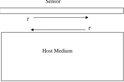
The considered system is a homogeneous and isotropic elastic medium, with a thin sheet of piezoelectric sensor surface-bonded to it. There is a deboned area (crack) along the interface between the medium and the sensor, as illustrated in Figure 3.1. The length of the crack is denoted as 2c, and the thickness of the sensor is denoted as h. In Figure 3.1, z axis is the poling direction of the sensor, in which electric field is usually applied or measured. The system is subjected to an oblique harmonic incident longitudinal wave with a frequency of ω_{and an} incident angle of θ₀. The horizontal displacement of the incident wave is given by )] cos sin ( exp[ ) , ( ₀ ₀ ₀ 0 t Kz Ky i A z y uy = ∗ θ + θ −ω (3.1)

(24)

where A0 denotes the magnitude of the displacement, and K =ω/cL is the wave number, with c being the longitudinal wave velocity. L

The steady state response of the system, including displacement, stress, and strain, will involve a time factor exp(−iωt). For example, the real displacement can be expressed as: ) exp( ) , ( ) , ( 0 0 t i z y u z y uy = y ⋅ −

ω

(3.2)

where u_y0(y,z) represents the real displacement field, and u0_y(y,z) represents the magnitude. Since exp(−iωt) exists in all parameters, for the purpose of convenience, in the following discussions, only the magnitudes of these field variables are used to represent these field variables.

This study will focus on a thin-sheet sensor, with relatively small thickness in comparison with its length and width. Here we only consider small debonding situation, in which the boundary condition at the ends of the sensor may be ignored, so the sensor can be assumed to be infinite in length. Therefore, the magnitude of axial stress s

y

σ and strain s y

ε can be assumed to be uniform across the thickness of the sensor, where the superscript ‘s’ represents the sensor. Because the thickness of the sensor used is very small compared with its length, the applied electric field will mainly result in a deformation along the longitudinal direction. Accordingly, the sensor can be modeled as an electroelastic line subjected to the applied electric field and a distributed longitudinal force, τ( y), as shown in Figure 3.2, where τ( y) is the interfacial shear stress transferred between the sensor and the host structure. The longitudinal displacements of the sensor and the host medium are represented by s

y

(25)

Figure 3.1: The geometry of the sensor system

Figure 3.2: The stress field of the sensor system θB B0B B Host Medium h y z Sensor Host Medium τ τ 2c

(26)

3.1.1 The Dynamic Sensor Model

3.1.1.1 Electromechanical Behavior of Piezoelectric Materials

When the piezoelectric material is subjected to a mechanical load, it will produce electric displacement; and conversely, strains can be generated when electric field is applied. The former property is used in sensing, and the electromechanical behavior of piezoelectric materials can be described as:

{ }

[ ]{ } [ ]{ }

{ }

D

[ ]{ } [ ]{ }

e E E e c λ ε ε σ − = − = (3.3)

where {

σ

},{

ε

},{D}_and{E}_{represent the magnitude of the stresses, the strains,} the electric displacement and the electric field intensity, respectively. [c is a ] matrix containing the elastic stiffness parameters for a constant electric potential,

]

[e represents the piezoelectric constants, and [λ] represents the dielectric constants for zero strains.

In the current study, for a surfaced bonded piezoelectric thin sheet with interfacial debonding, and the length of the interfacial crack is small compared with its width in the x-axis direction, it is more reasonable to consider the problem as a plane stain problem in y-z plane, which suggests that εx =0. The surface of the piezoelectric sensor will be traction free. Therefore, the following condition should be satisfied, 0 , 0 = = z x σ ε (3.4)

The stress component σy and the electric displacement D can be obtained by z substituting the above equation into the constitutive equation, and the results are as follows: z y z z y y E e c e e D E c c e e c c c     + +     − =       − −       − = 2 33 33 13 33 13 33 13 33 13 33 2 13 11 λ ε ε σ (3.5)

(27)

where c11, c13 and c33 are the elements of [c], e11_and e33 are the elements

of [e], and λ₃₃is the element of [λ].

Therefore, the constitutive relation of the piezoelectric material under plain deformation is given by z y z z y y E y u e D eE y u E λ σ + ∂ ∂ = − ∂ ∂ = (3.6)

with the small deformation assumption

y u_y y _∂ ∂ = ε (3.7)

The effective material constants of the piezoelectric materials can be expressed as

33 2 33 33 33 13 33 13 33 2 13 11 c e c c e e e c c c E − = − = − = λ λ (3.8)

3.1.1.2 The Current Sensor Model

Figure 3.3: The stress field inside the sensor

The attention will be focused on cases where high frequency electric field is applied, which results in wave propagation with the typical wave length comparable to the length of the interfacial crack. In this case, the inertia effect of the sensor must be considered. According to the current one-dimensional sensor

s y s y dσ σ + s y σ dy

τ

(28)

model, the equation of motion of the sensor based on the equilibrium of force can be expressed as 0 ) ( + 2 = + s y s s y u h y dy d ω ρ τ σ (3.9)

where the superscript and subscript ‘s’ represent the sensor, ρ_s is the mass density of the sensor, and s

y

σ represents the magnitude of the axial stress along the sensor as shown in Figure 3.3.

In addition, the sensor will operate in an open-loop mode with no external charge supplied to it. Therefore, the electric displacement across the sensor will be zero, as Dz = 0. By making use of Equation (3.6), the axial stress along the sensor σs_y

can also be expressed in terms of the axial displacement s y

u and the electric field z E as y u E s y s s y _∂ ∂ = σ (3.10) s

E is the effective modulus defined by

s s s s E e E λ 2 + = , (3.11)

where Es,es,λs are piezoelectric material parameters.

Substitute Equation (3.10) into Equation (3.9), the governing equation of the sensor can be rewritten as

0 ) ( 2 2 2 = + + ∂ ∂ h E y u k y u s s y s s y τ (3.12) where k_s is the wave number given by

s

s c

k =ω/ (3.13)

and c is the axial wave speed with a definition of s cs = Es /ρs .

(29)

Therefore, the axial displacement and strain of the sensor can be expressed in terms of the unknown shear stress

τ

_as:

) ( 2 s2 s s y k s h E u − = τ (3.15) τ ε ) ( 2 s2 s s y k s h E is − − = (3.16) where τ, uysand s y

ε represent the Fourier transform of τ( y), the Fourier transform of the axial displacement and the Fourier transform of the axial strain, respectively.

(30)

I

3.1.1.3 Dynamic behavior of the host medium

(a) (b) (c) Figure 3.4: The stress field inside the host medium

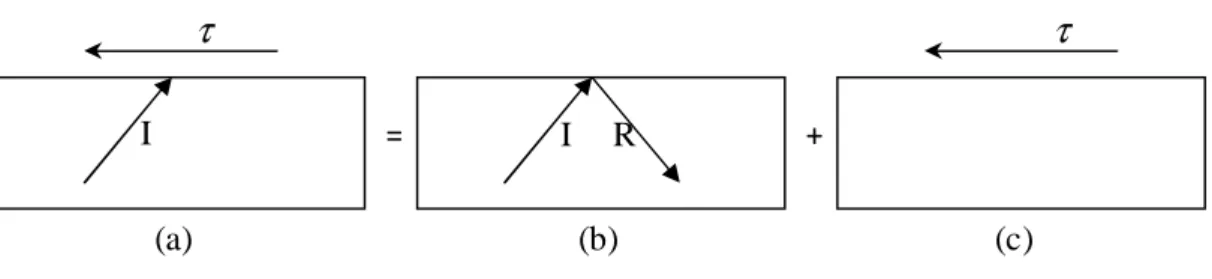
The host medium is subjected to an incident wave (I) and a surface shear stress

τ

, as shown in configuration (a) of Figure 3.4. The incident wave will be reflected to generate a reflected wave (R) and

τ

_{will generate a dynamic field in the medium.} Therefore, the stress field inside the host medium can be expressed by superimposing the configurations (b) and (c). The solution of configuration (b) can be obtained by using free-surface boundary conditions, and the corresponding displacement and strain field inside the host medium can be written as:

y ik I I y y ik I I y e A ik e A u 0 0 0 = = ε (3.17)

Here AI_and k₀ are the amplitude and the apparent wave number of the induced wave field in the configuration (b), which can be obtained by using equations (A.1) – (A.18) in Appendix A.

The unknown displacement in configuration (c) is denoted as u , which is τy

induced by the shear stress

τ

_{on the top surface of the host medium.}

The dynamic plane strain displacement field in a homogenous isotropic elastic medium is governed by the following equations [80]:

2 2 2 2+ Φ= ∇ + Ψ= ∇ = _I _R +

τ

I

(31)

in which the Laplacian operator ∇2_{stands for} ∂2/∂y2 +∂2/∂z2,

Φ

and Ψ are two complex potentials, and K =

ω

/c_L, k =ω/c_T are two wave numbers with

ω

, c_L and c_T_{being the circular frequency of the incident wave, the} dilatational and shear wave velocities, respectively. The non-vanishing displacement and stress components are

y z u z y uy z ∂ Ψ ∂ − ∂ Φ ∂ = ∂ Ψ ∂ + ∂ Φ ∂ = , (3.19)

The relevant stress components are

      ∂ Ψ ∂ − Ψ − ∂ ∂ Φ ∂ =       ∂ ∂ Ψ ∂ − ∂ Φ ∂ − Φ − =       ∂ ∂ Ψ ∂ + ∂ Φ ∂ − Φ − = 2 2 2 2 2 2 2 2 2 2 2 2 2 2 2 2 2 2 y k z y z y y k z y z k yz z y µ τ µ σ µ σ (3.20)

where

µ

is the shear modulus of the isotropic elastic solid.

Therefore, the general solution of the wave induced by the shear stress

τ

_{can be} determined by solving the governing equations by using the Fourier transform defined by Equation (3.14), which can be expressed as

z z e s B z s e s A z s, ) ( ) α , ( , ) ( ) β ( = Ψ = Φ (3.21)

From which the displacement components can be determined as

z z z z z y e s isB e s A u e s B e s isA u β α β α α β ) ( ) ( ) ( ) ( + = + − = (3.22)

where A(s) and B(s) are two unknown functions of s; and

α

,

β

are given by

k s k s s k i k s K s K s s K i K s < >     − − − = < >     − − − = | | | | , | | | | 2 2 2 2 2 2 2 2 β α (3.23) which ensure that the induced stress field satisfies the radiation condition of the problem at infinity.

The outgoing wave caused by

τ

_{in the host medium should satisfy the following} conditions along its surface,

(32)

0 , = − = z yz τ σ τ at z=0 (3.24)

Making use of the general solution of uy and uz and the boundary conditions, the unknown parameters A(s) and B(s) can be determined in terms of

τ

. Therefore, the Fourier transform of the dynamic displacement in the host medium

τ y u can be expressed by

[

z z

]

y s z s e s k e uτ α β µβ τ 2 2 2 2 ) 2 ( 2 ) , ( − − ∆ = (3.25) where 2 2 2 2αβ 4 ) 2 ( s −k − s = ∆ .

The Fourier transform of the dynamic stress field components cause by

τ

_{in the} host medium can be obtained as

[

]

[

]

[

z z

]

yz z z z z z y e k s e s z s e e k s is z s e k s e k is z s β α τ β α τ β α τ αβ τ τ β τ σ α β τ σ 2 2 2 2 2 2 2 2 2 2 ) 2 ( 4 ) , ( ) 2 ( 2 ) , ( ) 2 ( ) 2 ( 2 ) , ( − − ∆ = − − ∆ = − + + − ∆ = (3.26)

3.1.1.4. Perfectly Bonded Sensor

If the sensor is perfectly bonded to the host medium, at the upper surface of the host medium and the lower surface of the sensor, the displacement should be continuous, τ y I y s y u u u = + , at z = 0 (3.27)

By substituting Equation (3.15) and (3.25) into Equation (3.27), the Fourier transform of τ can be expressed as

) (s m u_yI = τ (3.28) where ∆ − − = µβ 2 2 2 ) ( 1 ) ( k k s h E s m s s .

(33)

) ( ) ( , ) ( ) ( 0 2 2 0 0 2 2 0 k m k Eh k k m k k h E u u s s I y s y s s I y s y = ₋ = ₋ ε ε (3.29) where I, y

u ε_yI are given by Equation (3.17), and k0 is the apparent wave

number of the incident wave.

3.1.1.5 Sensor System with Interfacial Debonding

If the sensor is not perfectly bonded to the host medium, the displacement field will be discontinuous along the interface between the sensor and the host medium. The displacement discontinuity can be expressed by the following dislocation density function:

[

]

0 ) ( = − − ∂ ∂ = z I y y s y u u u y y τ ϕ (3.30)

By applying Fourier transform we can get

[

]

₀ ) ( = − − − = z I y y s y u u u is s τ

ϕ

(3.31)

Therefore, the Fourier transform of the shear stress

τ

_{can be related to the} deformation, by substituting Equation (3.15) and (3.25) into (3.31), as follow:

) ( ) ( ) ( ) ( s s m s i s m u s I y ϕ τ ⋅ + = (3.32)

The interfacial crack is subjected to the following boundary conditions:

c y y u y u y u c y I y y s y = + ≥ < = ), 0 , ( ) 0 , ( ) 0 , ( , 0 τ τ (3.33) from which the interfacial shear stress

τ

can be determined.

By applying the inverse Fourier transform to Equation (3.32), the above boundary conditions can be expressed in terms of the following singular integral equations:

c y k m u dsd y s s m s d y I y c c c c _ − = <     − ⋅ + −

∫

₋

∫

₋ , ) ( )] ( sin[ ) ( 1 ) ( 0 ξ ξ λ ξ ξ ξ ϕ λ (3.34) and

∫

₋c = cϕ(ξ)dξ 0 (3.35)

(34)

where

λ

=

µ

/(1−v) is the limit of the kernel of the integration when s→+∞, which represents the singular behavior of the field.

Equations (3.34) and (3.35) can be solved by expanding

ϕ

(

ξ

) using Chebyshev polynomials as follow:

∑

∞ = − = 0 1 2/ 2 ) / ( ) ( j j j c c T C ξ ξ ξ ϕ (3.36)

where Tj are Chebyshev polynomials of the first kind and C are unknown j

constants. From the orthogonality conditions of the Chebyshev polynomials, Equation (3.35) reduces to C0 =0. Substituting (3.36) into (3.34) and making use of the following relations (p > 0):

n j n j p J d p T n j n j p J d p T j n j j n j 2 1 2 ) ( ) 1 ( 0 ) cos( 1 ) ( 2 1 2 0 ) ( ) 1 ( ) sin( 1 ) ( 1 1 2 1 1 2 = + =    − = − = + =    ₋ = −

∫

− − π ξ ξ ξ ξ π ξ ξ ξ ξ (3.37)

with Jj being Bessel functions of the first kind, the following algebraic equation

for Cj are obtained

c y k m u y f C c y U C j I y j j j j j < ⋅ = +      

∑

∞ = ∞ =1 − 1 0 1 , ) ( ) ( λ (3.38)

where Uj represent Chebyshev polynomials of the second kind with

       =       − ⋅ ⋅ − + =       − ⋅ ⋅ − =

∫

∞ + ∞ n j ds sy sc J s m s n j ds sy sc J s m s y f j n j n j 2 ) sin( ) ( 1 ) ( 1 ) 1 ( 1 2 ) cos( ) ( 1 ) ( 1 ) 1 ( ) ( 0 1 0 λ λ (3.39)

If the Chebyshev polynomials in Equation (3.36) are truncated to the Nth term and Equation (3.38) are satisfied at N collocation points given by

N l N l c y y l l , 1,2,..., 1 cos ~ _ ₌      + = = π (3.40)

(35)

N l j k m u y f C N l N jl C I y N j l j j N j j , , 1,2,..., ) ~ ( ~ ) ~ ( 1 sin 1 sin 0 1 1 = ⋅ = +       +       +

_∑

∑

= = _π λ π (3.41) where yI I y s s l k k s u y ,~,~,~,β~,~ ,ε~ ~ 0 are given by y k i I I y y k i I I y s s s s e k i c A e c A u k s sc s c k k c k k c y y ~ ~ 0 ~ ~ 2 2 2 0 0 0 0 ~ ~ ~ ~ ~ ~ , ~ , ~ , ~ , / ~ = = − = = = = = ε β (3.42)

By solving Equation (3.41), Cj(j=1,2,...N) can be determined. Therefore, the interfacial shear stress

τ

_{and the axial strain inside the sensor} εys can be

expressed as

[

]

        + ⋅ − =         + − ⋅ =

∑

= = N j j j s I y s y N j j j j I y y h C k m k k q y f y g C k m u 1 0 2 2 0 1 0 ) ~ ( ) ~ ( ) ~ ~ ( ~ ) ~ ( ) ~ ( ) ~ ( ~ λ ε πυ ε λ λ τ (3.43) where

[

]

      = ⋅ ⋅ − + = ⋅ ⋅ − =        =       − ⋅ ⋅ − + =       − ⋅ ⋅ − =      > − − − − < =

∫

∞ ∞ ∞ + ∞ − n j ds y s s J s m n j ds y s s J s m y h n j ds y s s J s m s n j ds y s s J s m s y f y y y y y y y y U y g j s n j s n j j n j n j j j j 2 ) ~ ~ cos( ) ~ ( ) ~ ( ~ 1 ) 1 ( 1 2 ) ~ ~ sin( ) ~ ( ) ~ ( ~ 1 ) 1 ( ) ~ ( 2 ) ~ ~ sin( ) ~ ( 1 ) ~ ( ~ 1 ) 1 ( 1 2 ) ~ ~ cos( ) ~ ( 1 ) ~ ( ~ 1 ) 1 ( ) ~ ( 1 ~ 1 ~ ) ~ sgn( ~ 1 ~ ) ~ sgn( 1 ~ ) ~ ( ) ~ ( 0 2 0 2 0 1 0 2 2 1 β λ β λ λ λ (3.44) with

(36)

s s v E E E q ) 1 ( 2 − 2 = =πλ π (3.45) h c / = υ (3.46)

3.2 Analysis and Discussion

This section will be devoted to the discussion of the dynamic load transfer from the host medium to the surface-bonded sensor under different geometric and loading conditions. A longitudinal wave will be introduced as the mechanical load, and numerical simulation will be conducted to investigate the effect of the following three parameters upon the strain distribution along the sensor: the loading frequency kc, the material combination factor q as defined in (3.45), and the crack geometry

υ

expressed by (3.46).

Two types of sensors are considered, lead zirconate titanate (PZT-4) and polyvinylidene fluoride (PVDF) sensors. The material constants of the PZT-4 sensor and the host medium are assumed to be [81]:

Sensor (PZT-4): . / 10 45 . 6 , / 10 45 . 6 , / 7 . 12 , / 1 . 15 , / 2 . 5 10 5 . 11 , 10 43 . 7 , 10 9 . 13 9 33 9 11 2 15 2 33 2 31 10 33 10 13 10 11 Vm C Vm C m C e m C e m C e Pa c Pa c Pa c − − ₌ _× × = = = − = × = × = × = λ λ Host Medium: . 3 . 0 , 10 74 . 2 × 10 = = Pa v E

It results in the material mismatch factor q = 0.54.

For the PVDF sensor and the host medium, the material constants are as follows [82], which leads to a value of q = 20.4.

Sensor (PVDF): 10 63 . 1 , 10 4 . 1 , 10 61 . 3 33 9 9 13 9 11 Pa c Pa c Pa c = × = × = ×

(37)

Host Medium: . 28 . 0 , 10 5 . 19 × 10 = = Pa v E

For the sake of convenience, in the following calculations, the incident angle of the incident longitudinal wave is chosen as o

30

0 =

θ ; Poisson’s ratio of the host medium v=0.3; the mass density of the sensor ρ_sand the host medium ρ_h is chosen as the same, ρs = ρh = 2700kg/m3 [79].

3.2.1 Model Validation

In order to validate the current model, the finite element method (FEM) has been used, based on the static coupled-field analysis performed by the ANSYS software, by using the following loading condition: in the interfacial deboning area along the interface between the sensor and the host medium, the distributed shear stress

τ

with a uniform magnitude is applied. In the FEM model, twenty nodes are created across the thickness of the sensor.

Figure 3.5 shows the magnitude of the longitudinal strain of the sensor s y

ε induced by

τ

along the interface between the sensor and the host medium, using the numerical method based on the current model, in comparison with the corresponding FEM results. Here the strain has been normalized by

0 * ε υ ε ε ⋅ = s y s y , with ) 1 ( 0 v + = µ τ

ε and υ =20.0 , where υ is defined by (3.46). The anisotropic elastic stiffness matrix components of the lead zirconate titanate (PZT-4) sensor are: Pa c Pa c Pa c Pa c Pa c Pa c 10 66 10 44 10 33 10 13 10 12 10 11 10 06 . 3 , 10 56 . 2 , 10 5 . 11 , 10 43 . 7 , 10 78 . 7 , 10 9 . 13 × = × = × = × = × = × =

The material constants of the host medium are [81]: E=2.74×1010Pa, v=0.3.

The main difference between these results occurs in the vicinity of the interfacial crack tips when y/c is close to -1, in which the mechanical field becomes complicated due to the high stress concentration. In other areas far away from the

(38)

crack tips, the difference is less than 2%. Therefore, the current model is validated and can be used for the current analysis.

-5 -4.5 -4 -3.5 -3 -2.5 -2 -1.5 -1 -0.5 0 -0.1 0 0.1 0.2 0.3 0.4 0.5 0.6 y/c A FEM results Numerical results Figure 3.5: Amplitude of εys* 3.2.2 Strain Distribution

As shown in Figure 3.3 (a), if there is no bonded sensor on the surface of the host structure, the strain field of the medium will be εIy( y). Because of the existence of sensor, the strain field in the medium will be disturbed by the electromechanical coupling between the host medium and the sensor. In order to study the relation between sensor response and the undisturbed deformation, the following dynamic strain ratio κ( y) is introduced:

, ) ( ) ( ) ( θ ε ε κ i I y s y Ae y y y = = (3.47)

where A and θ_{denote the amplitude and the phase angle of the dynamic strain} ratio.

The dynamic strain ratio represents the percentage of deformation transferred from the host medium to the sensor. It is an index of the sensing characteristics of

(39)

frequency upon it will be discussed. Special examples will be given in both perfect-bonding and imperfect-bonding cases.

3.2.2.1 Perfectly Bonded Piezoelectric Sensor

For the case of a perfectly-bonded sensor system which is subjected to an incident longitudinal wave as the mechanical load, the dynamic strain ratio is constant along the interface. The strain in the sensor is given by Equation (3.29), so the strain ratio can be obtained by substituting Equation (3.29) into (3.47),

0 0 2 2 2 0 0 2 2 0 ₁ ₍ ₎ 1 ) ( ) ( 1 ∆ − − = − = µβ κ k k k h E k m k k h E s s s s (3.48) where 2 0 2 2 0 2 2 0 2 2 2 0 0 2 0 2 0 = −i k −k ,∆ =(2k −k ) −4k k −k K −k β .

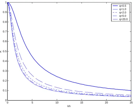
For the static case where the loading frequency k = k0 =ks =0, from Equation (3.48) we can obtain the strain ratio as 1. Figure 3.6 and Figure 3.7 show the influence of the loading frequency kh on the amplitude A and the phase angle θ of the dynamic strain ratio κ for the cases when q = 0.5, 1.0, 2.0, 5.0 and 20.0. With the increase of the loading frequency, the amplitude of the strain ratio decreases gradually. Besides, from Figure 3.6 and Figure 3.7 it can be observed that when q reaches 5.0 or higher, the curves are close and change with q insignificantly. The result indicates that, in the perfectly bonded case, the influence of the loading frequency on the load transfer is significant only when the loading frequency is very high. For relatively low frequency, kh < 1.0 for example, the change of A and θ in comparison with the static values is less than 5%.

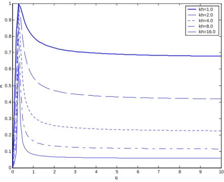
As defined in Equation (3.45), the material mismatch factor q is an index of the relative stiffness of the sensor, representing the material combination of the sensor and the host medium. Figure 3.8 and Figure 3.9 show how the amplitude and phase angle of the dynamic strain ratio change with the material combination factor q, with a series of kh values considered. From Figure 3.8 we can see that the amplitude of the dynamic strain ratio will increase to the maximum value 1.0, when q reaches a critical value qc about 0.3; and then diminish with the increase

(40)

of q. This critical value of qc is independent on the loading frequencies, and it is determined by the phase angle of the incident longitudinal wave and Poisson’s ratio, which can be expressed by solving the equation of κ =1:

2 sin ) 1 ( 2 2θ₀ π v qc = − ′ (3.49)

where θ0 is the incident angle of the incident longitudinal wave, and

v v v − = ′ 1 . For θ0 =30o and v=0.3, q c

= 0.31. From the figure we can also see that under the higher loading frequency condition, the material combination affects the dynamic load transfer more significantly.

(41)

0 5 10 15 20 25 0 0.1 0.2 0.3 0.4 0.5 0.6 0.7 0.8 0.9 1 kh A q=0.5 q=1.0 q=2.0 q=5.0 q=20.0

Figure 3.6: Amplitude of κ with different loading frequencies

0 5 10 15 20 25 0 10 20 30 40 50 60 70 80 90 kh T h e p h a s e a n g le o f th e s tr a in r a ti o q=0.5 q=1.0 q=2.0 q=5.0 q=20.0

(42)

0 1 2 3 4 5 6 7 8 9 10 0 0.1 0.2 0.3 0.4 0.5 0.6 0.7 0.8 0.9 1 q A kh=1.0 kh=2.0 kh=4.0 kh=8.0 kh=16.0

Figure 3.8: Amplitude of κ with different material combinations

0 1 2 3 4 5 6 7 8 9 10 -100 -80 -60 -40 -20 0 20 40 60 80 100 q T h e p h a s e a n g le o f th e s tr a in r a ti o kh=1.0 kh=2.0 kh=4.0 kh=8.0 kh=16.0

(43)

3.2.2.2 Interfacial Debonding

If the sensor is not perfectly bonded to the host structure, the interfacial defection will disturb the dynamic load transfer and consequently affect the performance of the piezoelectric sensor. The dynamic strain ratio will be dependent on the location along the interface, which can be expressed by using Equation (3.43) and (3.17): I y N j j jh y C y ε κ κ _~ ) ~ ( ) ~ ( 1

∑

= + = (3.50)

where κ is given by Equation (3.48), representing the strain ratio of the perfect bonding case. Cj are the coefficients of Chebyshev polynomials in Equation

(3.36), εyI

~ _and _h _(y~₎

j are given by Equation (3.42) and Equation (3.44),

respectively.

For the static case where k = k0 = ks= 0, the right hand side of Equation (3.41)

equals zero, so the coefficients Cj are zero as well, and κ in Equation (3.50)

becomes 1.Therefore, the strain ratio

κ

(y~)_{given by (3.50) becomes a constant} value

κ

(~y)=

κ

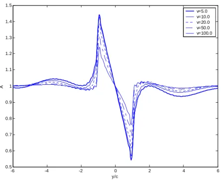
=1.

3.2.2.3 The Effect of the Loading Frequency

The loading frequency will have significant effects upon the load transfer between the sensor and the host structure. Three cases are considered with q = 0.5,

υ

= 5.0; q = 5.0,

υ

_{= 5.0; and q = 0.5,}

υ

_{= 20.0, which is given by Equation (3.46)} and (3.47). A series of the loading frequency (kc) values from kc = 0.0 to 8.0 are chosen to investigate the effect of different loading frequencies upon the strain distribution.

Figure 3.10 shows the amplitude A of the dynamic strain ratio

κ

(y~) under relatively low loading frequencies kc = 0.0, 0.4, 0.8, 1.2 and 2.0, with q = 0.5,

υ

= 5.0. Figure 3.11 shows the amplitude A of the dynamic strain ratio under relatively high loading frequencies kc = 0.0, 2.0, 4.0 and 8.0, with q = 0.5,

υ

=

University of Alberta