Working Paper No. 520
A forecast evaluation of expected equity
return measures
Michael Chin and Christopher Polk
January 2015
Working Paper No. 520
A forecast evaluation of expected equity return
measures
Michael Chin
(1)and Christopher Polk
(2)Abstract
Recent studies find evidence in favour of return predictability, and argue that their positive findings result from their ability to capture expected returns. We assess the forecasting performance of two popular approaches to estimating expected equity returns, a dividend discount model (DDM) commonly used to estimate ‘implied cost of capital’, and a vector autoregression (VAR) model commonly used to decompose equity returns. In line with recent evidence, in-sample tests show that both estimates generate substantially lower forecast errors compared to traditional predictor variables such as price-earnings ratios and dividend yields. Out-of-sample, the VAR and DDM estimates generate economically and statistically significant forecast improvements relative to a historical average benchmark. Our results tentatively suggest that the VAR approach better captures expected returns compared to the DDM.
Key words: Expected returns, implied cost of capital, dividend discount model, return predictability, forecasting.
JEL classification: G10, G11, G12, G17.
(1) Macro Financial Analysis Division, Bank of England. Email: [email protected] (2) Department of Finance, London School of Economics. Email: [email protected]
The views expressed in this paper are those of the authors, and do not necessarily reflect those of the Bank of England, the Monetary/Financial Policy Committees or the PRA Board. We would like to thank Katie Farrant, Andrew Meldrum, Simon Price, Chris Young and an anonymous referee for extensive and valuable comments. This paper was finalised on 18 December 2014.
The Bank of England’s working paper series is externally refereed. Information on the Bank’s working paper series can be found at www.bankofengland.co.uk/research/Pages/workingpapers/default.aspx
Publications Team, Bank of England, Threadneedle Street, London, EC2R 8AH
Summary
Central banks pay close attention to movements in equity prices, as they can have important implications for the real economy. For example, increases in equity prices may increase the value of individuals' investments and pensions, and can lower firms' cost of financing new projects, and these effects can lead to increases in aggregate consumption and investment. Understanding why equity prices have changed is also important. An investor who holds a firm's equity is entitled to a share of the profits that the firm generates in the immediate and distant future. In theory, this investor is therefore willing to pay a price for that equity that reflects expectations of these future cash flows (which are often dividend payments). At the same time, however, the equity price will not exactly equal the total expected future sum of dividends, since in general investors dislike having to wait for dividend payments, and also need to be
compensated for the possibility that dividends rise and fall depending on the future state of the economy. As a result, when evaluating the price of an equity, investors discount expected dividends by an additional amount reflecting the return on a safe asset and a premium for risk, which is the expected return.
At the aggregate level, expected returns are important equity market indicators, as they summarise the attitudes toward risk of a range of investors. But they cannot be observed directly, and one needs a model to estimate them. In theory, these expected return estimates should be able to forecast actual future returns on the stock market to an extent. Academics and practitioners have devoted substantial effort to testing whether equity returns are indeed
predictable, often using variables such as dividend-price and price-earnings ratios. Successes in this area have, in general, been attributed to the ability of a forecasting measure to capture expected returns. Put another way, the better the measure of expected return, the better that estimate should be at forecasting future returns.
Our paper focuses on two competing measures of expected returns, and examines their ability to forecast returns on the equity market. The first is estimated using Campbell's 1991 vector autoregression (VAR) model, a simple statistical model that describes the relationship between short-term returns and a range of other variables. These short-term dynamics can be used to make predictions about returns over longer horizons, and we use these as one measure of expected returns. The second measure is estimated using an adaptation of Gordon's 1962 dividend discount model (DDM). This approach directly models investor dividend expectations using analyst survey measures, and then solves for the expected return as the difference between these expectations and the equity price. We examine the ability of these measures to forecast future returns in a range of tests. In addition to the two models, we also consider a selection of popular variables used to forecast returns, and ask whether the expected return estimates forecast better compared to these predictors.
We use UK and US data to examine the forecasting performance of the range of variables over short and long forecast horizons (from three months to three years). We initially consider each forecasting variable individually, and run thorough statistical tests of their predictive power. Here, we find that the DDM and VAR expected return measures perform well, whereas the more traditional predictors do not. In a related test, we compare the relative accuracy of the
expected return measures to the traditional predictors, and find that the former generate much smaller errors when predicting returns. Finally, we consider how these predictors would have done in `real-time', where we imagine we had to generate forecasts on a month-by-month basis using only information available to us at the time of making each forecast. Previous work has found that forecasting performance is often very weak under these test conditions. In fact, in many cases, it has been shown that one can achieve better forecast performance by simply using the past average return on the market to predict its future direction. In contrast, we show that our expected returns estimates perform better compared to this simple rule, in particular when forecasting returns at longer horizons, which is strong evidence in favour of the approaches we consider.
1
Introduction
Many models have been used to understand movements in equity prices, and a large pro-portion of these rely on a present-value framework, where the equity price is expressed as the expected sum of its future cash flows discounted at an appropriate rate. This discount rate comprises a risk-free element and an equity risk premium, the compensation an investor requires to hold an equity, and is also known as the expected return on equity. The ex-pected return on the aggregate equity market is an important concept in asset pricing and macroeconomics, as it reflects perceptions of aggregate risk and risk-aversion, and is directly related to firms’ cost of capital and household wealth. Within the finance literature, ex-pected returns have been the focus of much theoretical and empirical work, where there is a lot of evidence to suggest that they vary substantially over time and play a large role in stock market movements (see Cochrane (2011)). Expected returns are unobservable, however, and need to be estimated.
A consequence of time-varying expected returns is that they allow for the presence of predictability within the equity market, and there is a large related literature examining aggregate return predictability. The existence of return predictability has been a somewhat controversial topic, where earlier positive findings have been challenged on the basis of is-sues regarding statistical inference in regression-based tests, and the (lack of) out-of-sample performance of forecasting models (Welch and Goyal (2008)). Recent studies, however, have provided evidence in favour of return predictability. Li, Ng and Swaminathan (2013) show that an expected return estimate, generated from an adaptation of the Dividend Discount Model (DDM) framework of Gordon (1962), out-performs a range of traditional forecast variables within in- and out-of-sample forecast tests. In addition, Rapach, Strauss and Zhou (2010) show substantial improvements in forecasting performance can be achieved through combining information contained in a range of individual predictor variables. The aforemen-tioned studies argue that the improvements in forecast performance arise due to the fact that their forecasting models better capture expected returns.
This paper considers two popular approaches to modelling expected equity returns. The
first approach also uses the Gordon (1962) DDM framework, in a similar formulation to that proposed in Li, Ng and Swaminathan (2013) and Chen, Da and Zhao (2013). This approach uses analyst forecasts of future dividends in a present-value formula, and solves for the expected return used to discount these cashflows by residual. The second approach models the short-run dynamics of equity returns in a Vector Autoregression (VAR), originally proposed in Campbell (1991), which is more commonly used to decompose equity returns
into cashflow and discount rate news. The discount rate news in these studies simply reflects changes to the expected return forecasts made by the VAR, and this expected return estimate is the focus of our study. The VAR approach can be thought of as combining information in a range of individual forecast variables. We use a standard VAR specification to generate expected return estimates, which closely resemble the models used in recent studies (e.g. Campbell and Vuolteenaho (2004), Campbell, Giglio and Polk (2013), Campbell, Giglio, Polk and Turley (2014)).
We test whether the expected return measures are able to forecast realised returns, both in- and out-of-sample, and compare their performance to a range of traditional predictor variables such as the price-earnings ratio and term spread, using UK and US data. The expected return measures perform favourably in simple forecast regression tests, where they significantly predict realised returns at a range of horizons, and where the traditional predic-tors generally do not. In-sample, the VAR and DDM estimates also generate substantially lower forecast errors compared to the alternative predictors. Out-of-sample, we compare the range of forecast variables to a historical average benchmark forecast, andfind that the VAR and DDM offer economically and statistically significant forecast improvements. In line with recent findings, we provide evidence that direct measures of expected returns perform well in forecast tests, and our paper generally provides evidence in favour of return predictability.
We also explore the relative performance of the VAR and DDM approaches in measuring expected returns. The VAR and DDM approaches are both housed within the present value framework, but the models differ in their estimation, where one chooses to model either cash
flows or discount rates as a residual. Since the DDM expected return is estimated by residual, it is important that the analyst forecast inputs, usually taken from I/B/E/S surveys, are well-measured. There are, however, well-known measurement issues and biases in I/B/E/S earnings forecasts, which have the potential to distort the expected return estimates. In particular, the surveys can be slow to update in response to news, and the forecasts can also be subject to large data corrections (Ljungqvist, Malloy and Marston (2009)). There are also potential limitations to the VAR approach, where this method may struggle to capture long-horizon expectations, and where outputs from this approach clearly depend on the variables included within the model. Within our in- and out-of-sample forecast evaluations, we attempt to explore the extent to which these issues are detrimental to the forecasting ability of these approaches. In-sample, we find that the VAR-based estimates generate substantially lower forecast errors compared to the DDM. Within the out-of-sample tests, however, the performances of the VAR model and DDM are harder to differentiate.
well as providing evidence on their relative forecasting performance, we also explore the re-turn decompositions from both models. Chen, Da and Zhao (2013), noting the limitations of the VAR and DDM approaches, use both approaches to decompose equity returns at thefirm and aggregate levels, andfind a much larger role for expected cashflows in return variation, relative to the preceding VAR and predictive regression-based evidence (e.g. Campbell and Ammer (1993), Ammer and Mei (1996), Vuolteenaho (2002)). We find that the DDM and VAR find similar relative roles for cashflow and discount rate news, though we show that they often differ in their interpretations of stock market movements at given points in time.
We also contribute to the return predictability literature by demonstrating that an al-ternative DDM expected return estimate also successfully predicts returns. While our DDM estimate closely resembles that used in Li, Ng and Swaminathan (2013), there are some differences compared to our model. First, the previous versions jointly model earnings fore-casts and ‘plowback’ rates — the proportion of earnings paid out as dividends in each period. We use I/B/E/S dividend forecasts directly, which removes the need to make any assump-tions about plowback rate expectaassump-tions, since these will already be captured in the dividend forecasts. Second, the previous versions use an expanding moving average of GDP growth rates as their long-term growth assumption, whereas we assume a constant long-run growth rate. While the differences are not large, we demonstrate that the forecasting performance is robust to changes in specification and a different forecast sample period. Finally, our application to UK data also adds to a relatively small literature decomposing UK equity returns (e.g. Cuthbertson, Hayes and Nitzsche (1999), Bredin, Hyde, Nitzsche and O’Reilly (2007)) and assessing return predictability in the UK (e.g. Wells and Wetherilt (2004), Price and Schleicher (2005)).
The paper proceeds as follows: Section 2 briefly outlines the theoretical foundations of the two approaches, and provides details of their empirical implementation. Section 3 examines the outputs and diagnostics of the models, and draws a comparison between the different approaches. Section 4 tests the ability of the models to predict future returns in and out of sample. Section 5 concludes.
2
Modelling Expected Equity Returns
2.1
VAR Model: Campbell (1991)
The VAR approach is associated with the return decomposition originally proposed in Camp-bell (1991). A log-linear approximation expresses unexpected returns in terms of revisions
to both expected future dividend growth and expected returns.1 +1−+1 ≈(+1−) ∞ X =0 ∆+1+ −(+1−) ∞ X =1 +1+ (1)
Here, +1 is the log total return from holding a stock from period to period + 1,
+1 is the log dividend paid during period , is a by-product of the log-linearization of
returns, defined as the ratio of steady-state prices to prices plus dividends, which empirically is a number a little less than one. is the conditional expectation formed at time , and
∆ denotes a one-period backward difference operator. We refer to the revisions to future dividends and expected returns as ‘cash flow news’ and ‘discount rate news’ respectively, and rewrite the identity using a tilde to denote revisions to each of the components:
e
+1=e+1−e+1 (2)
2.1.1 VAR Implementation
The empirical implementation of this framework requires a model for generating forecasts of dividends and returns. We follow a common approach and avoid modelling dividends, mod-elling only the expected return components in a VAR, and calculating revisions to expected dividends as the residual component of the identity in (2) (e.g. Campbell (1991), Campbell and Vuolteenaho (2004), Bernanke and Kuttner (2005), Campbell, Giglio and Polk (2013)).2
We define an -variable state vector +1, where the first element is the stock return +1.
We assume that +1 follows afirst-order VAR process:
+1 =+Γ++1 (3)
+1 is the -by-1 state vector, Γ is the -by- matrix of VAR coefficients, and +1 is
an i.i.d. -by-1 shock vector. The VAR model can be used to generate forecasts of single period returns at any point in the future, where the-period ahead return forecast is given by:
(+) = ( −Γ)(−Γ)+Γ (4)
Expected returns are generated for a range of horizons, where the -period expected return is the sum of the single-period log returns over the forecast horizon. These expected
1See Campbell and Shiller (1988) and Campbell (1991) for detailed derivations.
2This is motivated by the complications that arise when modelling the dividend growth process, which has a near unit root, exhibits strong seasonal variation, and is subject to changes in corporate pay-out policies.
return estimates are the subject of the forecast evaluation tests later on. One can use revisions to these forecasts from one period to the next as measures of the components of equation (2). Specifically, the left-hand side +1−+1 can be written as:
e
+1=e10+1 (5)
wheree1is thefirst column of a-by- identity matrix. Revisions to expected returns and dividends can be written as:
e
+1 =e10+1 (6)
e
+1 = (e10+e10)+1 (7)
where=Γ(−Γ)−1. In addition to the market return, we include variables in the VAR
that have been shown to forecast equity returns, and that are commonly used in applications of this framework (e.g. Campbell and Vuolteenaho (2004), Bernanke and Kuttner (2005), Campbell, Giglio and Polk (2013) and Campbell, Giglio, Polk and Turley (2014)). We include a smoothed dividend-price ratio, defined as the index price at time scaled by the trailing average of 10 year earnings (Campbell and Shiller (1988)). This ratio, or a close variant of it, is one of the most frequently used predictor variables within studies that implement the Campbell (1991) framework.3 We include the term spread, defined as the 10-year constant
maturity government bond yield less the yield on the 3-month Treasury bill (Keim and Stambaugh (1986)), also commonly used in related studies. In the US VAR, we include a default spread defined as the difference between BAA and AAA corporate bond yields. For the UK model, due to the short sample of available data for the UK default spread, we include a pay-out ratio, defined as the ratio of aggregate dividends paid to aggregate earnings over the past twelve months, another commonly used predictive variable (Lamont (1998)). This model ought to provide a good reflection of the VAR specifications that have been used in previous studies, though the model more closely resembles the specifications in Campbell and Vuolteenaho (2004), Campbell, Giglio and Polk (2013) and Campbell, Giglio, Polk and Turley (2014).
Recent evidence suggests that the inclusion of the price-dividend ratio and short-term interest rate capture a significant amount of the relevant information for modelling expected returns. Maio and Philip (2014) test the sensitivity of the return decomposition to the inclusion of a large amount of information extracted from alternative macroeconomic and
3As described in Campbell and Ammer (1993) and Engsted, Pederson and Tanggaard (2012), it is crucial that a stock price variable is included within the VAR, since this is an underlying assumption used to derive the Campbell (1991) framework. The inclusion of the price-earnings ratio ensures that this condition is met.
financial variables. Theyfind that there is little incremental information in the extra series, over and above the dividend yield and short-term interest rate. To the extent that our VAR specification includes information contained in both of these predictor variables, we might take some reassurance that our model provides a reasonable representation of the market’s information set, given that one can only ever hope to capture a subset of this information.
2.2
Dividend Discount Model
The common starting point of the DDM approach is the approximation of the standard present value equation. The standard two-period equation is as follows:
= ∙ +1++1 1 + ¸ (8)
Here is the index price in month,[+1]is the dividend forecast for year + 1, and
is the cost of capital. This can be extended to an infinite horizon model, which rules out
the existence of bubbles:
= ∞ X =1 + (1 ++) (9)
The DDM approach is then a special case of the infinite horizon present value equation, which makes the further assumption that expected returns are a deterministic constant, and allows the expectations operator to be moved inside the summation sign — applying only to future dividends: = ∞ X =1 (+) (1 +) (10)
There are many ways to implement this version of the model empirically. The majority of applications, however, tend to explicitly model the path of expected dividends over two to three years from period. We use the following adaptation:4
= 5 X =1 (+) (1 +) + (+6) (1 +)5(−) (11)
Dividends from + 1 to + 4 are measured using I/B/E/S survey data. Specifically, we use aggregate I/B/E/S growth rate forecasts for years 1 to 3 to calculate the level of expected dividends over these three years.5 We then assume that year 4 earnings grow at
4This is a similar model to that used in Inkinen, Stringa and Voutsinou (2010).
the average of the year 3 growth rate and the I/B/E/S medium term growth rate. Year 6 growth is set equal to a long-run growth assumption of 5%, which allows calculation of a perpetuity starting at this point in time.6 The final Year 6 cash flow is valued using the
constant growth perpetuity formula, hence the appearance of(−)in the denominator of
thefinal cashflow. By assuming that the discount rate is constant at each maturity, we can solve for the implied discount rate numerically.
Our model closely resembles that used in Chen, Da and Zhao (2013) and Li, Ng and Swaminathan (2013), which in turn are based on the formulation of Pastor, Sinha and Swaminathan (2008), though there are some differences compared to our model. First, the other versions jointly model earnings forecasts and ‘plowback’ rates — the proportion of earnings paid out as dividends in each period. We use dividend forecasts directly, which removes the need to make any assumptions about plowback rate expectations, since these will already be captured in the I/B/E/S dividend forecasts. Second, whereas our long-term growth rate is constant, the previous versions use an expanding moving average of GDP growth rates. In practice, this difference does not materially affect the DDM estimate. Since the expanding moving average is based on growth rates over a long history (since 1930), the long-term growth rate over our sample (1998—2014) changes little. As a result, changes in the discount rates are almost perfectly correlated (0.99). There is a small difference in the levels of the constant and average long-term growth rates, which generates a small level difference between the discount rate estimates under the two different assumptions.
2.2.1 Dividend Discount Model: Cash flow and Discount Rate News
Following Chen, Da and Zhao (2013), we estimate the impact of revisions to cash flow and discount rates on equity returns, allowing a comparison of ‘news’ series with the outputs from the VAR decomposition. The -period return from holding an equity, excluding dividends, is equal to the change in price over this period, divided by the price in period :
+ = µ +− ¶ (12)
Within the present value framework, the equity price can be expressed in terms of
ex-firm forecasts in the present value formula to estimatefirm level expected returns, and calculate the aggregate expected return from these values. We use aggregate forecasts in the present value formula to estimate aggregate expected returns directly.
6The expected return estimate is only sensitive to the long-run growth assumption in the level. Roughly speaking, a 100 basis point increase in the long-run assumption increases the estimate by around 80 basis points. Estimates under different growth assumptions are almost perfectly correlated, however (0.99 or greater when varying the assumption from 1-10%).
pected dividends and expected returns at time and +: = ∞ X =1 (+) (1 +) =( ) (13) + = ∞ X =1 +(++) (1 ++) =(+ +) (14) + = µ (+ +)−( ) ¶ (15)
where represents the stream of expected future dividends, and represents the future
path of expected returns. Returns can be decomposed into cashflow and discount rate news as follows: + = 05 µ (++)−( +) +(+)−( ) ¶ (16) + = 05 µ ( +)−( ) +(+ +)−(+ ) ¶ (17) + = + + + (18)
These ‘news’ series do not correspond exactly to those obtained through the VAR decom-position. The Campbell (1991) framework is a decomposition of unexpected return, which also includes dividend payments. In contrast, the DDM decomposition decomposes price changes i.e. excluding dividends, and is not relative to an expectation. These differences should not materially affect a comparison between the two models, for two reasons. First, there is a lot of noise in short-term return variation, implying that returns are difficult to forecast, and that most of return variation is unexpected. Second, as pointed out in Chen, Da and Zhao (2013), dividends play a minor role in total return volatility. Over the period 1965 to 2013, the standard deviation of monthly total returns on indices in the UK and US are 5.55% and 4.51%, respectively. These numbers are little affected when excluding dividends, where the UK and US standard deviations are 5.52% and 4.50%, respectively.7
2.3
Data
The data that enter the VAR are obtained from Global Financial Data (GFD). The data are monthly frequency, and values are taken at the end of the month. Returns are calculated
7And the series are near perfectly correlated, with correlation coefficients of 0.97 and 0.99 for the UK and US respectively.
from total return equity indices for the FTSE All-Share and the S&P 500, where returns on these indices include reinvested dividend payments from constituentfirms. Within the VAR, and also within the forecast tests, we use Price-Earnings (PE) ratios, Dividend-Price (DP) ratios and 10-year and 3-month Treasury bill rates for the UK and US, provided by GFD. PE and DP ratios are based on 12 month trailing earnings and dividends respectively, and these ratios are used to calculate the smoothed Price-Earnings ratios and payout ratio. We use I/B/E/S analyst forecasts in the DDM, which are obtained from Datastream. Due to the short sample of I/B/E/S data, our forecast tests are limited to data from August 1998 to December 2013, while the variables that enter the VAR estimations and other predictive regressions are available further back in time. For the UK, our sample starts in January 1965 and ends in December 2013. For the US, we use data from January 1978 to December 2013.
3
Expected Return and News Estimates
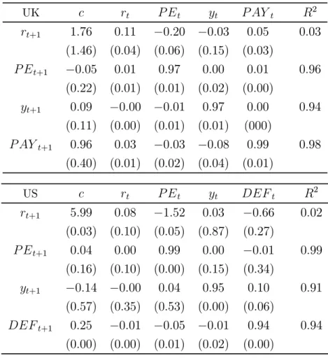
The results from the UK and US VAR models are provided in Table A1 in the appendix. The coefficient estimates in the returns equation are in line with what one might expect, and with past evidence. For both the UK and US, there is a small degree of momentum in short-term returns, shown by the positive coefficient on the lagged return. The price-earnings ratios and default spread negatively predict returns, and the pay-out ratio has a positive coefficient.8
3.1
Expected Returns
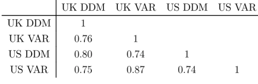
As outlined in the previous section, the VAR model and DDM can be used to generate estimates of expected returns. The DDM assumes that expected returns are constant across horizons, while the VAR allows for variation in expected returns at different horizons. Figures A1 and A2 show the expected return estimates from the two models for the UK and US. It is not immediately obvious which horizon estimate from the VAR should be compared against the DDM estimate, though since the DDM can be thought of as averaging across short to very long horizons, we opt for the 10-year expected return estimate from the VAR. Visually, the two measures are comparable. Broadly speaking, the series increase around 2002 and 2008, consistent with the equity market falls and economic slowdowns around these periods. Table A2 shows that the estimates co-move strongly across models and across countries. When comparing the two estimates for the same country, the correlation between
8For the lagged return, see Conrad and Kaul (1998), for the price-earnings ratio, see Campbell and Shiller (1988), for the payout ratio see Lamont (1998)
the DDM and VAR estimates is 0.75 for the UK, and 0.74 for the US. When comparing across countries, we observe a high degree of international co-movement. The correlation between UK and US estimates is in excess of 0.7, regardless of which model we use. While the levels of the UK and US VAR estimates are similar, the level of the UK DDM estimate is around 2 percentage points higher than the US DDM estimate on average.9
3.2
Cash
fl
ow and discount rate news
Using the methods described earlier, we decompose monthly returns into their cash flow and discount rate components, and investigate the role of each component in explaining the variance of returns. For both models, the variance decomposition is obtained using the following identity, which expresses return variance as a function of the cashflow and discount rate news series:
() =( ) +( ) 1 = µ ( ) () ¶ + µ ( ) () ¶ (19)
The relative proportions can therefore be obtained from the OLS regression coefficients of equity returns regressed on the DDM news series, and the regression coefficients of unex-pected returns regressed on the news components from the VAR model. Table A3 reports the return variance decomposition from the two models. The implications of the two models are broadly consistent: discount rate variation tends to account for a larger proportion of return variance, in line with past evidence. The distinction between discount rate and cash
flow news is less marked for the US VAR model, however. The results are consistent with Chen, Da and Zhao (2013), who find a qualitatively similar role for cash flow and discount news at the 12-month horizon between the two model types.
The return decompositions are shown in Figures A3 and A4. Each series has been smoothed using a 12-month moving average, and the discount rate news series has been inverted, such that negative contributions correspond to higher discount rates. Focusing on the stock market downturn over 2000-02, we observe slightly different interpretations of market movements. The VAR decompositions attribute a large part of the stock market declines around 2002 to downward revisions to expectations of future cash flows, although
9This may reflect differences in payout policies between UK and US equity markets, wherefirms in the US market have a greater tendency to return profits to shareholders through share repurchases, rather than dividends. All else equal, this would result in a lower level of forecasted dividends in the US market, which reduces the estimated expected return.
they also assign some role to higher discount rates. While the US DDM decomposition tells a similar story, showing a large negative contribution from cashflow news in 2001, the UK DDM decomposition points to discount rates as the main driver (perhaps intuitive given the smaller economic slowdown that the UK experienced over this period). The UK DDM decomposition is more consistent with the results of Campbell, Giglio and Polk (2013), who use the VAR framework, and also attribute most of the downturn in the early 2000s to higher discount rates. The other decompositions are consistent with Garrett and Priestly (2012), however, who explicitly model revisions to cash flow forecasts in the VAR framework, and
find significant negative cash flow news in the early 2000s stock market decline. At the height of the 2007-09 financial crisis, all models attribute the stock market declines to a combination of negative cash flow and discount rate news, consistent with both Campbell, Giglio and Polk (2013) and Garrett and Priestly (2012). The DDM decompositions, while attributing declines to cashflow news eventually, interpret the large initial falls as reflecting large upward revisions to discount rates.
One of the primary concerns regarding the I/B/E/S data is the potential for relatively long lags between relevant information being released and the forecasts being updated. Fig-ure A5 shows a comparison between the cashflow news estimates from the VAR and DDM models, and realised dividend growth 12 months ahead. While the two cash flow news se-ries cannot be considered direct forecasts of future dividend growth, one would still expect to see correlation between these measures and realised future dividends. The broad trends are similar, however there are clear differences in timing of large movements and of higher frequency variation. In particular, the fall in actual dividends over 2008 was a little better predicted by the cash flow news series estimated from the VAR, suggesting that the VAR cash flow news series may contain more timely information about future dividends. This observation may confirm the issue of lags in I/B/E/S survey updates, and motivates a more systematic evaluation of the ability of these models to capture expectations, which is the focus of the next section.
4
Forecast Tests
In this section, we evaluate the forecasting performance of the DDM and VAR model, fo-cusing on the expected return estimates the models generate. We do this by testing the ability of the estimates to forecast realised future returns, using common forecast evalua-tion frameworks (e.g. Welch and Goyal (2008) and Campbell and Thompson (2008)). We also consider the forecasting performance of each model relative to a range of alternative
predictor variables that are commonly assessed in the return predictability literature, in-cluding: the dividend-price ratio (DP), three price-earnings measures (a 12 month trailing ratio ‘PE’, a cyclically adjusted ratio ‘PES’ and a forward looking ratio ‘PEF’), and default and term spreads (‘DEF’ and ‘TERM’), further details for which can be found in Table A4 in the appendix. In general, we refer to this set of forecast variables as the ‘alternative’ or ‘traditional’ predictors. Summary statistics are provided in Table A5.
Early evidence on return predictability suggested that each of the traditional predictor variables were able to forecast future returns (see Rozeff (1984), Fama and French (1988), Fama and French (1989)). These findings were later challenged, however, on the basis of issues regarding statistical inference in regression-based tests, that led to results that were biased towardfinding predictability (Stambaugh (1999)). An additional challenge came from Welch and Goyal (2008), who showed that these forecasting models performed poorly out-of-sample. In theory, price-dividend and price-earnings ratio variables ought to be able to forecast returns to the extent that they capture expected returns. These ratio variables are not clean measures of expected returns, however, as expected dividend growth is also a potentially important component that has distortionary effects (Lettau and Ludvigson (2005)). One would prefer to consider an equity price relative to its future earnings, though the denominators of these ratios are usually backward looking. In this sense, one might expect the DDM-implied expected return to provide a better estimate of expected returns, and therefore better forecast future returns. Indeed, Li, Ng and Swaminathan (2013) show that a range of DDM expected return estimates outperform standard ratio and business cy-cle variables using US data. Their results complement studies emphasizing the importance of modelling expected cash flow growth components of price ratio variables, and showing enhanced forecasting performance once this is accounted for (e.g. Lacerda and Santa-Clara (2010) and Golez (2014)). The VAR methodology may also provide an improvement upon single predictor variables, to the extent that the model combines information from a range of predictor variables in a parsimonious manner to generate return forecasts. In some cases it has been shown that poor performance of individual forecasting variables can be improved upon by forming combination forecasts based on the individual predictors or separate fore-casts, for example in stock return prediction (Rapach, Strauss and Zhou (2010)) and in studies forecasting output and inflation (Stock and Watson (2003)). The VAR does not combine forecasts in the same way as these studies, which often use weighting methodologies that are based on recent forecasting performance, but incorporates a handful of predictor variables nonetheless.
other predictors can forecast future returns using in-sample regressions. We then proceed to compare the VAR and DDM with each other and the alternative predictors. Finally, we explore the sample forecastability of the range of predictors. Within the out-of-sample analysis, we test the forecasts from the DDM and VAR model against one another, and against a historical average benchmark.
4.1
In-Sample Prediction
We explore the in-sample relationship between the set of predictor variables and realised future returns using a standard framework. We estimate forecast regressions with average
-period returns as the dependent variable regressed on individual predictors at time :
+
=+++ (20)
where is the forecast horizon in months, and is the predictor variable. The -period
return is calculated as the cumulative sum of the monthly total log returns over the forecast horizon. The regressions are estimated for = 3, 12,24 and36-month horizons.
An issue when considering multi-period returns is that overlapping observations in the regression model induce serial correlation in the residual term. To correct for this issue in inference tests, we use Newey-West standard errors with+1lags. In addition, a well-known issue with this predictive regression set-up is that in-sample tests are biased in small sam-ples with persistent predictors, and when the predictor and return innovations are correlated (Stambaugh (1999)). To account for this bias, we follow a bootstrapping procedure similar to the one used in Rapach and Wohar (2005) and Neely, Rapach, Tu and Zhou (2014). This approach involves estimating a data generating process for single-period returns,+1, under
the null hypothesis of no predictability.10 We also estimate an autoregressive process for the
predictor variable, , and combine the return and predictor processes to generate a range
of pseudo-samples.11 These samples are generated by randomly drawing (with replacement) from the sets of residuals from the two processes. We generate 2000 samples, and construct empirical distributions of Newey-West -statistics by running predictive regressions over the relevant horizon for each pseudo-sample. We summarise results using -values based on a comparison of the Newey-West statistic from the regression based on the original data com-pared to the estimated empirical distribution.12 The significance of the coefficient estimates
10In applying this procedure and the null of no predictability, we abstract from the presence of predictability in the VAR-based expected return estimate.
11The AR lag-length is selected using AIC, where we consider up to a maximum of four lags. 12We conduct a one-sided test, where the -value for
0 ( 0) reflects the proportion of
gives a simple indication of the ability of each variable to predict future returns.
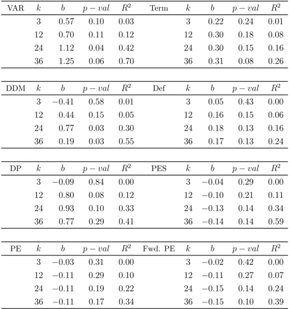
The results for the UK and US are provided in Tables 1a and 1b. For each predictor, the coefficient estimates are in the second column, -values in the third column, and the adjusted 2 in the fourth column. In general, across the range of predictors and forecast
horizons there are relatively few examples of statistically significant relationships. Popular forecast variables, such as the simple and forward looking price-earnings ratios show little predictive power over this period, in both the UK and US. There are some examples of significant relationships (at the 10% level) for the UK and US term spreads at the 24- and 36-month horizons, and the US default spread and smoothed price-earnings ratio also at longer horizons (consistent with the predictive power of these variables shown in Campbell and Vuolteenaho (2004), Campbell, Giglio and Polk (2013), and Campbell, Giglio, Polk and Turley (2014)).
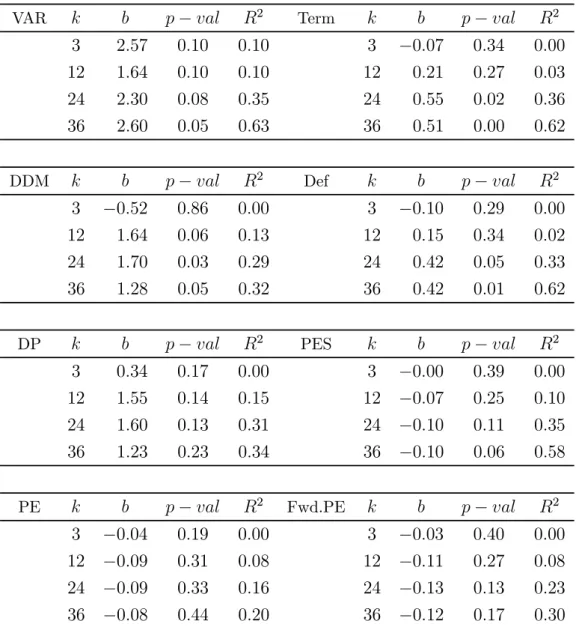
Turning to the model-based estimates, we find some evidence that the VAR and DDM significantly predict realised returns over this period. The UK and US VAR estimates are the only forecast variables that significantly predict 3-month returns at the 10% significance level, and the predictive power appears to also extend to longer forecast horizons, where the 12- to 36-month forecasts are significant in both the UK and US. The DDM does not display the same forecasting ability at short horizons, where the 3-month relationship is insignificant and predicts with the incorrect sign. On the other hand, however, the DDM significantly predicts 24- and 36-month returns at or below the 5% level in both the UK and the US, and 12-month returns in the US at the 10% level. The results are in line with Li, Ng and Swaminathan (2013), who run similar forecast regressions over an earlier sample using US data. They show that a similar DDM measure can significantly forecast returns, and that a range of ratio variables cannot except for a few cases at long horizons. The results suggest that the VAR and DDM differ in their forecasting ability depending on the forecast horizon. The DDM appears to perform better at long horizons rather than short, while the VAR appears to outperform others at shorter horizons. This difference in performance could arise naturally from the underlying assumptions of both models. When assuming constant expected returns in the DDM, it appears that the resulting estimate better captures long-horizon expected returns. To the extent that the assumption implies that the constant return estimate averages across expected returns over short to long (in fact, infinite) horizons, it is intuitive that the average maturity of this estimate is longer rather than shorter. Since the VAR is a model of the short-run dynamics of returns, one might expect it to perform well in forecasting shorter horizon returns, though our results suggest it also performs well at longer horizons.
Table 1a: Forecast Regressions: UK
The -period horizon return is regressed on the predictor variable, using OLS: +
= +
++. Sample period from August 1998 to December 2013. -values based on Newey-West t-statistics (with lag length+ 1), compared with bootstrapped empirical distributions.
VAR − 2 Term − 2 3 057 010 003 3 022 024 001 12 070 011 012 12 030 018 008 24 112 004 042 24 030 015 016 36 125 006 070 36 031 008 026 DDM − 2 Def − 2 3 −041 058 001 3 005 043 000 12 044 015 005 12 016 015 006 24 077 003 030 24 018 013 016 36 019 003 055 36 017 013 024 DP − 2 PES − 2 3 −009 084 000 3 −004 029 000 12 080 008 012 12 −010 021 011 24 093 010 033 24 −013 014 034 36 077 029 041 36 −014 014 059 PE − 2 Fwd. PE − 2 3 −003 031 000 3 −002 042 000 12 −011 029 010 12 −011 027 007 24 −011 019 022 24 −015 014 024 36 −011 017 034 36 −015 010 039
Table 1b: Forecast Regressions: US
The -period horizon return is regressed on the predictor variable, using OLS: +
= +
++. Sample period from August 1998 to December 2013. -values based on Newey-West t-statistics (with lag length+ 1), compared with bootstrapped empirical distributions.
VAR − 2 Term − 2 3 257 010 010 3 −007 034 000 12 164 010 010 12 021 027 003 24 230 008 035 24 055 002 036 36 260 005 063 36 051 000 062 DDM − 2 Def − 2 3 −052 086 000 3 −010 029 000 12 164 006 013 12 015 034 002 24 170 003 029 24 042 005 033 36 128 005 032 36 042 001 062 DP − 2 PES − 2 3 034 017 000 3 −000 039 000 12 155 014 015 12 −007 025 010 24 160 013 031 24 −010 011 035 36 123 023 034 36 −010 006 058 PE − 2 Fwd.PE − 2 3 −004 019 000 3 −003 040 000 12 −009 031 008 12 −011 027 008 24 −009 033 016 24 −013 013 023 36 −008 044 020 36 −012 017 030
The results also suggest differences in performance between the model-based estimates and the range of the alternative predictors, where commonly used ratio and business cycle variables struggle to forecast returns. We explore the performance of the VAR and DDM relative to each other, and to the alternative predictors on a pair-by-pair basis. We summarise the relative forecast errors from each model with a standard 2 statistic (e.g. Welch and
gives the ratio of forecast errors from two competing forecasting regressions: 2 = 1− µP =1(+−b+)2 P =1(+−e+)2 ¶ (21) b
ande are thefitted return projections from two competing forecasting models. When
2
0, thebmodel outperforms the benchmarkemodel. Statistical significance is assessed
with the Diebold-Mariano (1995) test. Table 2a shows the 2
values for the UK. In Panel
A the VAR is set as the benchmark model. 2 0 implies that the VAR underperforms the alternative predictor. In Panel B the DDM is the benchmark model (e), where 2 0
implies that the DDM underperforms.
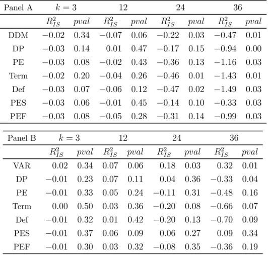
Table 2a: In-sample Relative Forecasting Performance — UK
Panel A shows the relative forecast errors with the VAR as the benchmark. Panel B shows the relative performance where the DDM is used as the benchmark. p-values are based on the Diebold-Mariano (1995) test, adjusted for serial correlation using a −1 lag parameter.
Panel A = 3 12 24 36 2 2 2 2 DDM −002 034 −007 006 −022 003 −047 001 DP −003 014 001 047 −017 015 −094 000 PE −003 008 −002 043 −036 013 −116 003 Term −002 020 −004 026 −046 001 −143 001 Def −003 007 −006 012 −047 002 −149 003 PES −003 006 −001 045 −014 010 −033 003 PEF −003 008 −005 028 −031 014 −099 003 Panel B = 3 12 24 36 2 2 2 2 VAR 002 034 007 006 018 003 032 001 DP −001 023 007 011 004 036 −033 004 PE −001 033 005 024 −011 031 −048 016 Term 000 050 003 036 −020 008 −066 007 Def −001 032 001 042 −020 013 −070 009 PES −001 037 006 009 006 027 009 034 PEF −001 030 003 032 −008 035 −036 019
For the UK, the negative2
values in Panel A indicate that the VAR generates smaller
forecast errors relative to all the other predictors considered, and across almost every forecast horizon. This outperformance is statistically significant at the 10% level in many cases, and is particularly marked at the 36-month horizon. Thefirst rows of results in both panels compare the performance of the VAR model and DDM. The results show that the VAR estimates perform significantly better compared to the DDM at the 12- to 36-month horizons. The DDM also generates smaller forecast errors in many cases, though statistically significant outperformance is less widespread compared to the VAR, and is concentrated at longer horizons, consistent with the simple regression results. Table 2b shows the results for the US.
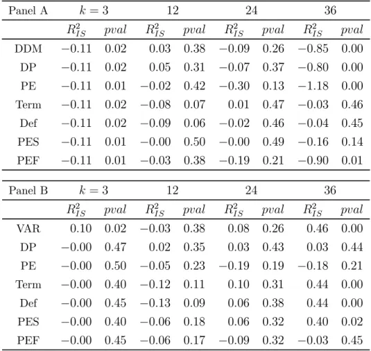
Table 2b: In-sample Relative Forecasting Performance — US
Panel A shows the relative forecast errors with the VAR as the benchmark. Panel B shows the relative performance where the DDM is used as the benchmark. p-values are based on the Diebold-Mariano (1995) test, adjusted for serial correlation using a −1 lag parameter.
Panel A = 3 12 24 36 2 2 2 2 DDM −011 002 003 038 −009 026 −085 000 DP −011 002 005 031 −007 037 −080 000 PE −011 001 −002 042 −030 013 −118 000 Term −011 002 −008 007 001 047 −003 046 Def −011 002 −009 006 −002 046 −004 045 PES −011 001 −000 050 −000 049 −016 014 PEF −011 001 −003 038 −019 021 −090 001 Panel B = 3 12 24 36 2 2 2 2 VAR 010 002 −003 038 008 026 046 000 DP −000 047 002 035 003 043 003 044 PE −000 050 −005 023 −019 019 −018 021 Term −000 040 −012 011 010 031 044 000 Def −000 045 −013 009 006 038 044 000 PES −000 040 −006 018 006 032 040 002 PEF −000 045 −006 017 −009 032 −003 045
2
values are negative, and statistically significant in many cases. The DDM also
outper-forms the alternative predictors in many cases, though the DDM significantly underperforms a handful of alternative predictors at the 36-month horizon. Overall, the assessment of rel-ative forecasting performance is less indicrel-ative of the VAR and DDM performing differently based on the forecast horizon, where the VAR generates significantly lower forecast errors at both short and long horizons.
To further explore the relative forecasting ability of the VAR and DDM estimates. We consider a multiple regression that includes only the model-based predictors, where we regress
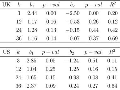
-period returns on the VAR and DDM estimates. The results are shown in Table 3. For the UK, both the VAR and DDM significantly predict 3-month returns. At 3-, 12- and 24-month horizons, the DDM forecasts have an incorrect sign. For the US, the VAR significantly predicts 3-month returns, while the DDM forecast is insignificant at this horizon and predicts with the incorrect sign. At the 24-month horizon, the DDM predicts significantly at the 10% level. These results mildly suggest that the VAR and DDM estimates contain information relevant for future returns at different horizons.
Table 3: VAR vs. DDM In-sample Relative Forecasting Performance
Parameter estimates for in-sample forecast regressions for the UK (top panel) and the US (bottom panel), estimated using OLS. The -period horizon return is regressed on the VAR and DDM expected returns: +
= +1
+2++. The sample period is from August 1998 to December 2013. -values based on Newey-West standard errors, with lag length set to + 1,compared with bootstrapped empirical distributions.
UK 1 − 2 − 2 3 244 000 −250 000 020 12 117 016 −053 026 012 24 128 013 −015 044 042 36 116 014 007 037 069 US 1 − 2 − 2 3 285 005 −124 051 011 12 104 025 125 016 015 24 165 015 098 008 041 36 237 009 024 027 064
Finally, we consider a multiple regression that relaxes the VAR specification, and tests the forecasting ability of the variables that are used to generate VAR expected return
es-timates. The multiple regression results for the UK and US are shown in Tables A6a and A6b in the appendix. For the UK, the price-earnings and payout ratio significantly predict returns, without imposing the parametric assumptions of the VAR. For the US, all variables are generally unable to predict returns, which suggests, given the results presented earlier, that modelling the short-run dynamics of these variables in a VAR provides incremental forecasting power.
Overall, the in-sample evidence suggests that the model-based expected return estimates are able to forecast returns, and in many cases outperform commonly used forecast variables. Given that the DDM can forecast returns and performs better than many other predictors, it appears that any biases or lags in the I/B/E/S analyst forecasts are not entirely detrimental to the DDM estimate. The in-sample results favour the VAR estimates over the DDM, however, where the VAR generates significantly lower forecast errors. It could be the case that I/B/E/S data imperfections underlie the underperformance of the DDM relative to the VAR.
4.2
Out-of-sample Prediction
The in-sample tests suggest that the VAR and DDM expected return estimates can predict future returns in many cases, as can some traditional predictors as certain horizons. The parameters of the in-sample forecast regressions, however, do not take into account whether information is available contemporaneously, and incorporate data ahead of time. This is a well-known limitation of in-sample tests. In this section, we proceed to run out-of-sample tests, which indicate whether the range of forecast variables would have been able to predict returns in real-time. We follow a standard out-of-sample testing procedure that evaluates forecasting performance where only contemporaneously available information is incorporated (e.g. Welch and Goyal (2008), Campbell and Thompson (2008), Rapach, Strauss and Zhou (2010)). Using a similar predictive regression framework to the in-sample analysis:
+=+++ (22)
we now estimate initial regressions based on data up to August 1998 (the first observa-tions), so that the first out-of-sample forecast is given by:
b
following which the data set is expanded by a single observation, and the model parameters re-estimated, such that the next out-of-sample forecast is given by:
b
+1+=b+1+b+1+1 (24)
This process is repeated to generate a set of out-of-sample forecasts at various horizons, from August 1998 to December 2013. To compare forecasting performance, we once again use the relative2 measure, which has the same interpretation as before, though is denoted
as 2
to identify it as the out-of-sample statistic:
2 = 1− µP =1(+−b+)2 P =1(+−e+)2 ¶ (25)
It is also the case in the in-sample exercise that the VAR expected return estimates are generated using information not available at the time, and so we need to re-estimate the model to account for this. Following the same methodology as outlined above, we expand the sample period of the VAR one period at a time and re-estimate the VAR model parameters and projections at each period. The DDM return estimates do not need to be re-estimated at this stage, since all the inputs to the model (in particular the survey forecasts) are available contemporaneously.
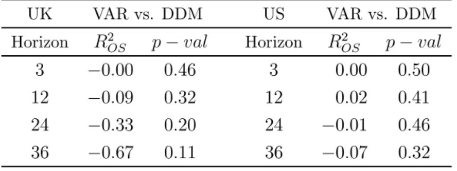
Wefirst compare the out-of-sample performance of the DDM relative to the VAR model, where the 2 values (with the VAR estimate as the benchmark) are shown in Table 4.
The negative2
values suggest that the VAR forecasts again generate lower forecast errors
in most cases, across the UK and US. In contrast with the in-sample results, however, the difference in predictive ability is not statistically significant. This suggests that the stronger performance of the VAR in-sample partly resulted from the look-ahead bias in its return projections.
Table 4: Out-of-sample forecasting performance: VAR vs. DDM
p-values based on the Diebold-Mariano (1995) test
UK VAR vs. DDM US VAR vs. DDM Horizon 2 − Horizon 2 − 3 −000 046 3 000 050 12 −009 032 12 002 041 24 −033 020 24 −001 046 36 −067 011 36 −007 032
To explore the out-of-sample forecasts further, we compare the forecasting performance of the range of predictors against a historical average benchmark + =
P
=1. As
sum-marised in Welch and Goyal (2008) and Campbell and Thompson (2008), this benchmark has been surprisingly difficult to beat in predicting returns. We again rely on the 2
to
summarise relative forecast errors, with the historical average as the benchmark. We for-mally test the reduction in the mean squared prediction error using the Clark and West (2007) test, where the test statistic is defined as:
+1 = (+−e+)2−[(+−b+)2−(e+−b+)2] b
+ is the forecast from the prediction model, and e+ is the benchmark average
forecast. The test statistic, +1, is regressed on a constant, and the Newey-West-statistic
is used to calculate the associated-value using a standard normal distribution. Comparisons against the historical average are based on the Clark and West (2007) test since the historical average model is nested within the predictive regression models. We continue to use the Diebold and Mariano (1995) test for the VAR and DDM, however, as we use the expected return estimates directly from these models rather than using the regression framework.
The comparison of each predictor against the historical average benchmark is shown in Tables 5 and 6 for the UK and US respectively. Here, a positive 2
value indicates that
the predictor outperforms the historical average.
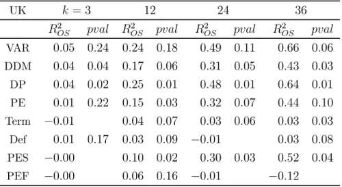
Table 5: Out-of-sample forecasting performance against historical average benchmark: UK UK = 3 12 24 36 2 2 2 2 VAR 005 024 024 018 049 011 066 006 DDM 004 004 017 006 031 005 043 003 DP 004 002 025 001 048 001 064 001 PE 001 022 015 003 032 007 044 010 Term −001 004 007 003 006 003 003 Def 001 017 003 009 −001 003 008 PES −000 010 002 030 003 052 004 PEF −000 006 016 −001 −012
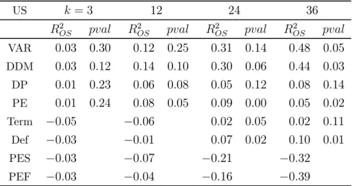
Table 6: Out-of-sample forecasting performance against historical average benchmark: US US = 3 12 24 36 2 2 2 2 VAR 003 030 012 025 031 014 048 005 DDM 003 012 014 010 030 006 044 003 DP 001 023 006 008 005 012 008 014 PE 001 024 008 005 009 000 005 002 Term −005 −006 002 005 002 011 Def −003 −001 007 002 010 001 PES −003 −007 −021 −032 PEF −003 −004 −016 −039
For both the UK and US, the VAR and DDM estimates perform well relative to the historical average, where the 2 values are positive and economically significant at most
forecast horizons. The DP and PE predictors also generate smaller forecast errors relative to the benchmark across all forecast horizons. For the UK, the magnitude of the reduction in forecast errors is comparable across the predictors, though only the DDM and dividend-price ratio generate statistically significant reductions at the 5% level for the majority of cases. For the US, the improvements relative to the historical average are most marked for the VAR and DDM, though the level of significance varies a little. The relatively weaker performance of the US ratio and business cycle variables is in line with past evidence (e.g. Welch and Goyal (2008), Li, Ng and Swaminathan (2013)). The relatively strong performance of the DDM is again consistent with Li, Ng and Swaminathan (2013), who show similar findings for the US at the 1-month horizon, using a 2-year moving average of their DDM estimate. The additional contribution of our findings is to show that the out-of-sample predictability extends far beyond the 1-month horizon, and remains when using the contemporaneous DDM estimate rather than the moving average.
As outlined earlier, the DDM and VAR may offer improvements upon traditional predic-tor variables to the extent that they better account for cashflow expectations, and combine information contained in a range of model inputs. The larger reduction in forecast er-rors of the two models in the US suggests that this extra sophistication does indeed lead to forecast improvements. This is less the case in the UK, however, where dividend-price and price-earnings ratios perform similarly well against the historical average. Overall, the out-of-sample analysis provides evidence in favour of return predictability, and provides
ad-ditional support to recent studies showing enhanced forecast performance using implied cost of capital measures and combined forecasts.
5
Conclusion
We test whether two expected equity return estimates can forecast realised returns. Expected returns are generated using two popular equity modelling approaches, which have been used in a variety of applications. Thefirst approach is the VAR model associated with Campbell (1991), and the second the Dividend Discount Model (DDM) adaptation of Gordon (1962), which has recently been used in Li, Ng and Swaminathan (2013) and Chen, Da and Zhao (2013). We examine the predictive power of these estimates in a range of in- and out-of-sample tests, and also consider their forecasting performance against commonly used predictors such as the dividend-price ratio and term spread. In-sample, wefind evidence that both the expected return measures can significantly forecast returns, whereas the traditional predictors generally can to a lesser extent. When exploring the relative performance further, wefind that the VAR-based estimate generates substantially lower forecast errors compared to the DDM estimate and the traditional predictors. Within the out-of-sample tests, there is further evidence that the model-based estimates are useful for forecasting, though the performances of the VAR model and DDM are harder to differentiate. We compare the range of forecast variables to a historical average benchmark forecast, andfind that the VAR and DDM offer economically and statistically significant forecast improvements.
6
Appendix
Table A1: UK and US VAR Results
VAR parameter estimates for the UK and US, estimated using OLS. The model is a first order VAR with a constant, that includes the market return , the smoothed price-earnings ratio , the term spread , and the default spread for the US and the pay-out ratio for the UK. Standard errors are shown in parentheses. The sample periods are January 1970 to December 2013 for the UK VAR and January 1977 to December 2013 for the US VAR. UK 2 +1 176 011 −020 −003 005 003 (146) (004) (006) (015) (003) +1 −005 001 097 000 001 096 (022) (001) (001) (002) (000) +1 009 −000 −001 097 000 094 (011) (000) (001) (001) (000) +1 096 003 −003 −008 099 098 (040) (001) (002) (004) (001) US 2 +1 599 008 −152 003 −066 002 (003) (010) (005) (087) (027) +1 004 000 099 000 −001 099 (016) (010) (000) (015) (034) +1 −014 −000 004 095 010 091 (057) (035) (053) (000) (006) +1 025 −001 −005 −001 094 094 (000) (000) (001) (002) (000)
Table A2: Expected return correlations UK DDM UK VAR US DDM US VAR UK DDM 1 UK VAR 076 1 US DDM 080 074 1 US VAR 075 087 074 1
Table A3: Return variance decomposition using VAR and DDM
e e VAR UK 034 066 US 043 057 DDM UK 026 074 US 038 062
Table A4: Alternative Predictor Variable Descriptions
Predictor Description
12 month Dividend-Price Dividends paid over the previous 12 months, divided by today’s price
12 month Price-Earnings Today’s price divided by earnings paid over the previous 12 months
Cyclically Adjusted Price-Earnings Today’s price divided by a 10 year trailing moving average of earnings
Forward Price-Earnings Today’s price divided by I/B/E/S ana-lyst forecasts of earnings over the next 12 months
Term Spread Yield on 10 year government bond less rate on 3 month Treasury Bill
Default Spread Yield on BAA-rated corporate bond basket less yield on AAA-rated basket
Table A5a: Forecast Variable Summary Statistics: UK
Predictor Mean Standard Deviation
VAR (3 month) 687 996 VAR (6 month) 724 960 VAR (12 month) 787 875 VAR (24 month) 895 725 VAR (36 month) 981 609 DDM 920 071 12 month Dividend-Price 325 061 12 month Price-Earnings 1528 424
Cyclically Adjusted Price-Earnings 1699 455
Forward Price-Earnings 1348 338
Term Spread 076 135
Default Spread 219 218
Table A5b: Forecast Variable Summary Statistics: US
Predictor Mean Standard Deviation
VAR (3 month) 800 438 VAR (6 month) 811 406 VAR (12 month) 827 378 VAR (24 month) 846 339 VAR (36 month) 855 307 DDM 743 034 12 month Dividend-Price 174 040 12 month Price-Earnings 2035 490
Cyclically Adjusted Price-Earnings 2341 646
Forward Price-Earnings 1650 392
Term Spread 186 121
Table A6a: Multiple regression: UK VAR variables
Parameter estimates for in-sample forecast regressions estimated using OLS. The-period hori-zon return is regressed on the variables that enter into the UK VAR:
+
=+1+2 +3+4 ++
The sample period is from August 1965 to December 2013. -values based on Newey-West t-statistics, based on lag length+ 1,compared with bootstrapped empirical distributions.
1 2 3 4 2
3 035 020 −013 005 002 041 159 011 033 12 010 023 −018 001 001 044 173 010 023 24 005 025 −019 003 −005 040 178 006 042 36 003 003 −017 002 −001 048 140 009 056
Table A6b: Multiple regression: US VAR variables
Parameter estimates for in-sample forecast regressions estimated using OLS. The-period hori-zon return is regressed on the variables that enter into the US VAR:
+
=+1+2 +3+4++
The sample period is from January 1977 to December 2013. -values based on Newey-West t-statistics, based on lag length+ 1,compared with bootstrapped empirical distributions.
1 2 3 4 2
3 035 059 −075 028 010 046 −261 032 034 12 010 041 −105 040 016 042 −254 033 016 24 005 052 −118 037 025 031 −466 019 025 36 004 009 −122 027 036 029 −573 015 039
Figure A1: Model-based Measures of UK Expected Returns 98 00 01 02 03 04 05 07 08 09 10 11 12 13 4 6 8 10 12 14 16 18 20 Per cent
VAR 10 Year Expected Return (UK)
98 00 01 02 03 04 05 07 08 09 10 11 12 13 6 7 8 9 10 11 12 Per cent
Figure A2: Model-based Measures of US Expected Returns 98 00 01 02 03 04 05 07 08 09 10 11 12 13 2 4 6 8 10 12 14 16 Per cent
VAR 10 Year Expected Return (US)
98 00 01 02 03 04 05 07 08 09 10 11 12 13 6 6.5 7 7.5 8 8.5 9 Per cent