The Game of Blackjack and Analysis of Counting Cards
Ariell Zimran, Anna Klis, Alejandra Fuster and Christopher Rivelli
December 2, 2009
Abstract
In this paper, we examine the game of Blackjack as the interaction of a gameplay decision and a betting decision. We specifically look at the role of card counting in these decisions. In the first half of the paper, we discuss how the game is structured, and therefore what optimal strategies can be used to increase expected payoff. We do this through a review of literature on the subject, as well as construction and analysis of a simplified version of Blackjack. We see that card counting greatly increases expected payoff. We also examine the costs of card counting, as well as the strategic interaction of a card counting player and the casino in which he is playing. Finally, we propose possible extensions of our work in the form of new areas that command further research interest.
1
Introduction
In recent years, card counting in Blackjack has become of increasing interest to the general public. Movies such as Rain Man,21 andThe Hangover have popularized the notion that tracking the number of “high” and “low” cards in play guarantees a high-payoff; but is this always the case? Are there situations in which counting can actually result in a lower payoff for the player? Furthermore, in each of these movies, the characters who count cards are extremely gifted: inRain Man as well asThe Hangover, the counters are genius savants, and in21, the counters are all students from MIT. As new technology comes on to the market that can help anyone become a card counter, such as applications for iPhones that count cards for the user, the costs of counting cards may increase due to more stringent casino policies. Thus, do individuals who are
not geniuses—or “mediocre card-counters”—really gain from keeping a count, or can it actually put them at a disadvantage?
In order to answer these questions, we must proceed step by step. This paper explores the basics of modeling Blackjack with game theory and then analyzes the costs and benefits of counting cards while playing the game. In section 2, we begin by looking at the optimum strategies in a simplified game of
our own design, similar to Blackjack. In the section 3 we review strategies for Blackjack discussed in the literature and the mechanics of card counting. In section 4 we present our model of the costs involved with card-counting. Section 5 demonstrates a C++ program for cost-benefit analysis of card counting. Section 6 offers possible expansions on the subject of Blackjack and card counting, such as false signaling, team strategy, and absent-mindedness. Section 7 concludes.
2
A Simplified Version of Blackjack
Before examining the game of Blackjack, it is beneficial to study the optimum strategies of a simpler game resembling Blackjack. Thus, we introduce the game ofSix.
2.1
The Game of Six
InSix, there are six cards: three high cards each of value equal to three and three low cards each of value equal to one. One card is dealt to player A, and then one card is dealt to player B. Another card is given to player A, and another to player B. All cards are visible, and there are only two cards remain to be dealt. Each player has one chance to choose whether to “hit”—receive one more card—or to “stay”—not take another card The object is to obtain the amount of points closest to six, and since each player can have at most three cards, the only way to achieve six is with two threes. Numbers higher than six (seven and nine are possible) are a “bust,” ending the game and giving an automatic victory to the player that did not bust. Player B can be considered a “dealer.” If he wins, he receives a payoff ofxfrom player A. Player A can be considered a “gambler.” If he wins, he receives a payoff 2xfrom player B. If the two players tie (the only possible tie is if both have a three and a one and neither chooses to “hit”) then neither receives anything and neither pays anything. The game can therefore be represented as follows:
• The set of players: {Athe “gambler”,B the “dealer”};
• The set of actions: {hit, stay}; and
• The set of payoffs:
– VA(win) = 2x – VB(win) =x – VA(lose) =−x – VB(lose) =−2x – VA(tie) =V(tie) = 0.
2.2
Outcomes and Optimum Strategies in Six
There are fourteen possible ways for the cards to be dealt, as demonstrated in Figure 8 in Appendix A. However, there are only four distinct cases that require different strategies. We denote the numerical value of playeri’s cards byni fori∈ {a, b}. If we adopt the rule that if a player is indifferent among two outcomes he will choose to “stay,” then we can solve for both players’ optimal strategy sets in each of the four cases. 1. nA= 6 ornB = 6. Many of the numerical outcomes are trivial because one player receives two threes, immediately having a six and winning the game. The player withn= 6 will certainly choose “stay,” as adding another card—be it a three or a one—would bust the player. The other player will also choose stay, since he cannot hope to match the first player’s six with only one more card. Thus, for any deal that gives one player two threes, the equilibrium is (stay, stay).
2. nA = 2 and nB = 4. If one player’s number is two and the other’s is four, then all the low cards of value equal to one have been dealt. The last two cards are threes. Thus, the player with n= 4 will want to stay, as a three would give himn= 7 and bust him. The player withn= 2 will want another card, as a three will give him n = 5 and allow him to win. In this case of nA = 2 and nB = 4, the equilibrium is (hit, stay).
3. nA= 4 and nB = 2. This case is similar to the previous case. The equilibrium is (stay, hit).
4. nA=nB= 4. This case is the most interesting in the game, as the remaining cards are a three and a one and the outcome of the game greatly depends on which card is first. The set up is seen in Figure 9 in Appendix A.
Firstly, A must decide whether to hit or stay. If he hits, he will receive either a three or a one. If he receives the three, playerAbusts withnA= 7, and the game ends with playerB winning. If playerA receives the one, thennA = 5 and playerA wins no matter if playerB stays or hits and receives the remaining three. Thus, player B will choose “stay” if playerAhits and receives a one.
If playerA were to stay, then player B must choose whether to hit or stay. If he hits, he will receive either the three or the one, with similar consequences as A faced. Since the probability of receiving either is p= 1
2, B’s expected payoff from hitting is
x
2. IfB stays when A stays, the players tie and
both receive a payoff of 0. Since 0>−x
2,B will choose stay. Thus, playerB has a dominant strategy
to “stay” if both players’ card values are four.
If playerAstays, playerB will also stay, and so playerAwill receive a payoff of 0. If playerAhits, he has a chance of busting and a chance of winning, both with probability p= 12. Thus, hitting givesA
an expected value of x2. Since x2 >0,Awill choose to hit.
In this case, the effect of non-symmetric payoffs is best visible. Player A, as the “gambler,” receives a higher payoff from winning than player B, the “dealer.” PlayerB, on the other hand, risks more in losing, and thus plays it safe. This is equivalent to most casino strategies. The equilibrium in this case is (hit, stay).
If the final decision to hit or stay were simultaneous then perhaps some randomization would be observed. However, because the game is sequential and cards are visible, there is no mixed strategy of randomization.
The optimal strategies for six are as follows:
• Player A: {ifnA = 6 ornB = 6 play stay; ifnA= 2 andnB = 4 play hit; ifnA= 4 andnB = 2 play stay; ifnA=nB = 4 play hit}.
• Player B: {ifnA= 6 or nB= 6 play stay; ifnA= 2 andnB= 4 play stay; ifnA= 4 andnB= 2 play hit; ifnA=nB=4 play stay}.
2.3
Expanding Six’s Strategies to Blackjack
Expanding the game ofSix makes it resemble Blackjack to a greater extent. The game of Blackjack can be played with one deck of 52 playing cards or with more than one (as is generally the case in Las Vegas). The object of the game is the get closer to 21 points than the dealer does without going over, or busting. All number cards are worth their face value; face cards (jack, queen, and king) are each worth 10 points. An ace is worth 11 points or one point, depending on which is best for the player. The dealer gives each player a card, and then places one card face up for himself. Then the dealer gives out a second card to each player, and places one card face down for himself. The players must then decide whether to “hit” or to “stay.” If a player hits, he receives another card; if he stays, then he receives no more cards. A player can hit multiple times. The players are not playing against each other - only against the dealer. However, the information provided by others’ cards is useful and can be taken into account, as all cards of the players are visible on the table.
Backwards induction did point to a feasibly describable equilibrium strategy set in the simple game of
Six. Attempting to apply a similar method to solve for the complete strategy set in Blackjack would be folly in length and purpose, as the game is repeated numerous times. Even a diagram of one hand, in which two cards are known, is expansive and inconclusive (see Figure 9 in Appendix A). Nevertheless, this inability of backwards induction to aid us in developing the complete strategy set for Blackjack is ultimately of no
consequence. In recent years, economists have developed computer programs that can be used to determine the “best strategy” sets for different types of players; most notable are the works of Baldwin et al. (1956), Thorp (1961), Thorp (1969) and Dubner (in Patterson, 2002).
3
Optimal Strategies of Blackjack
3.1
Literature Review
In the first real attempt to determine the best strategy for “Las Vegas” Blackjack, authors Baldwin, et al. (1956) begin by identifying two types of hands a player can hold. In the first type—a “regular hand”— the total of the player’s cards takes on one value less than or equal to 21. In the second type—a “soft hand”—the player draws one or more aces, and her cards can take on two or more distinct values less than or equal to 21.
Much of the article is spent deriving an equation for the expected value of the player’s total,x, given the dealer’s face-up card,D. This expected value,E(x, D), is then compared to the expected value of drawing one additional card, α, given D. The equation, however, is not nearly as interesting to the player as the concept behind it: if the player is able to calculate the expected payoff of “stay” and the expected payoff of “hit,” she is able to choose the action that maximizes her expected payoff.
Ultimately, the authors describe the optimum strategy of Blackjack as follows:1
M(D) = 13 D= 2,3 12 D= 4,5,6 17 D≥7, D= (1,11) M∗(D) = 18 D≤8,(1,11), D= (1,11) 19 D= 9,10
“LetDbe the numerical value of the dealer’s up card. D= 2,3. . .11[1,11]. LetM(D) be an integer such that if the dealer’s up card isDand the player’s total is unique and less thanM(D), the player should draw [or hit]; while if the player’s total is unique and greater or equal toM(D), the player should stay. . . Let us defineM∗(D) in the same way for soft hands with the understanding that player’s total means the larger of the two possible totals. . . [t]he optimum strategy was developed under the assumption that the player does not have the time or inclination to utilize the information available in the hands of the players preceding him in the draw” (Baldwin, et al. 1956).
1The authors also go into detail about when to double down and when to split. For the purposes of this paper, we will
According to this strategy, if the player initially draws a 6 and an 8 (for a total of 14) and the dealer’s up card is a Queen, the player should choose to hit.
Thorp (1961) takes the ideas originally set forth by Baldwin, et al. (1956), and expands upon them. While his predecessors assume that the player does not have “the time or inclination” to keep track of the cards that are in play or have been played, Thorp’s model assumes that the player is able to factor the cards that are currently in play (or those that are no longer in the deck) into their calculation of expected value. He asserts that, with this enhanced knowledge, it is possible to more precisely calculate the expected value of “hit” and “stay,” and consequently, increase one’s expected payoff.
Whereas Baldwin, et al. (1956) provide a simple model with an equally simple list of best strategies, Thorp’s model is substantially more complicated. As a result, it requires a set of best strategies that is also substantially more complicated. As Thorp writes, “A standard deck of cards has approximately 3.4·107
subsets, or possible combinations of cards that have been removed from the deck, “which are distinguishable under the rules of Blackjack. Using a computer program, Thorp calculates the expected value of “hit” and “stay” for each of these numerous subsets; while there are far too many to address within the context of his paper, Thorp uses the subsetQ(5) = 0 to demonstrate how his strategy functions:
“LetQ(I) be the number of cards of valueI. . . Suppose that just before a particular deal the player sees that all fives have been used (so that the unseen cards are a subset of that subset which we describe by
Q(5) = 0) and that the unused portion of the deck is ample for that deal. . . If Q(5) [does not equal] 0, the player bets the minimum allowed amount,m, merely to remain in the game and follows the complete deck strategy given by Baldwin et al. [(1956)] WhenQ(5) = 0 (and the remainder of the deck will suffice for the next deal), the situation has turned in favor of the player. He now bets a large amount, M, and uses the computed strategy forQ(5) = 0” (Thorp 1961).
The strategy of this subset as originally demonstrated by Thorp (1961) is demonstrated in Figure 11 in Appendix A.
The major advantage of Thorp’s (1961) model in comparison to that of Baldwin, et al. (1956) is that it increases the player’s expected value of playing Blackjack from −.62% to−.21%, a clear improvement. However, as previously stated, Thorp’s (1961) model is also far more complicated—it requires the player to remember the best strategies for thousands of possible subsets, which is not realistic for the vast majority of people. Furthermore, neither Thorp (1961) nor his predecessors consider the idea that players may be able to remember cards that were dealt in previous rounds, a strategy commonly known as “card counting.”
3.2
The Rules of Card Counting
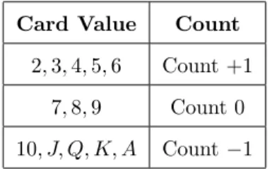
Harvey Dubner introduced a simplified variation of Thorp’s strategy, called the “Hi-Lo card counting strat-egy” (or the “point count system”), at the Fall Joint Computer Conference in Las Vegas in 1963 (Patterson 2002). His strategy works as follows:
First, the player must assign a particular value to each card as they are dealt:
Card Value Count
2,3,4,5,6 Count +1 7,8,9 Count 0
10, J, Q, K, A Count−1
Figure 1: A framework for card counting.
As Figure 1 demonstrates, cards 2, 3, 4, 5 and 6 are valued at plus one; cards 7, 8 and 9 are valued at 0; and cards 10, J, Q, K and A are valued at minus one. As the cards are dealt, the player keeps a “count.” The higher the count, the more likely it is that the player will get “Blackjack” (21 points in two cards) or that the dealer will bust, leading the player’s expected value to be positive. When the count is low, on the other hand, there are comparatively more “low” cards in play than “high” cards; the player no longer has an advantage over the dealer, and as a result, his expected value is negative. Thus, when the count is “high,” the player will place large bets, whereas when the count is low, the player will place the minimum bet possible (“Blackjack Strategy”, 2009).
4
The Decision to Count Cards
As the literature shows, keeping a count of the cards dealt during a particular hand and adjusting bets accordingly increases the player’s expected payoff for the hand. It is trivial to extend this logic to a series of hands during which the player keeps the count of cards and makes large bets when the count is positive. Following such a strategy would increase the player’s expected payoff for the duration of his play. However, a number of complications befall a player attempting to count cards. Many casinos, recognizing the fact that players who count cards are likely to win money at the casino’s expense, forbid gamblers from counting cards and punish those caught doing so with violence. Additionally, counting cards is not a simple task. Successfully keeping the count of a game of blackjack requires immense intellectual fortitude and players who attempt to do so are prone to errors that may lead them to lose money. This section presents several models analyzing a player’s decision to count cards in his interaction with a casino.
4.1
A Simple Model
First, we consider a strategic form game with perfect information.2 This game is defined by the set of players
P ={Player, Casino},
the set of actions for the player,
Ap={Count Cards, Fixed Strategy}, and the set of actions for the casino
Ac ={Observe, Not Observe}.
If the player chooses to count cards, he receives a payoff of 0 if he is observed counting cards, and a payoff of a if he is not observed. If the player chooses not to count cards, he receives a payoff of b regardless of whether or not he is observed. Leta > b >0.
If the casino chooses to observe the player, it must incur a fixed cost F.3 The casino also suffers losses
in the amount of the player’s winnings. The game is therefore as in Figure 2.
Player
Casino
O N
C 0,−F a,−a
S b,−F−b b,−b
Figure 2: The simple game
Two cases are of interest in this model.4
i. F ≥a. In this case the only equilibrium is in pure strategies: (C, N). This result is intuitive. If the cost of observation exceeds the loss from not observing, the casino will choose not to observe the players, and the player will take advantage of the lack of supervision to count cards.
2The models presented in this section can also be considered in sequential form; however, we have elected to model these
games in strategic form due to the fact that while the player and casino may make their decisions at different points in time, it is often difficult for each party to observe the other’s action.
3Practically, this cost is associated with the employment of security personnel, the installation of monitoring equipment to
observe gamblers as they play, and the time that must be devoted to observing and punishing a suspected card counter.
ii. F < a. In this case, there are no pure strategy Nash equilibria. The only equilibrium is in mixed strategies in which the player chooses to count cards with probability
q= F
a
and the casino chooses to observe with probability
r=a−b
a .
4.2
The Casino’s Type is Unknown
We have seen that the solutions of the simple game in subsection 4.1 are dependent on the relative values ofF and a. We now consider a model in which the casino may be one of two different types. The player’s perception of the probability of facing each type of casino is a determining factor of the equilibria of the game.
Suppose that the cost of observation, F, satisfies
F ∈ {FL, FH},
whereFL < a≤FH. Suppose that if the casino is vigilant it hasF=FLand that if it is not vigilant, it has
F =FH. The casino knows whether or not it is vigilant, and the player believes that the casino is vigilant with probabilityp. The game can therefore be modeled as in Figure 3.
Player Casino O N C 0,−FL a,−a S b,−FL−b b,−b Vigiliant (Probabilityp) Player Casino O N C 0,−FH a,−a S b,−FH−b b,−b
Not Vigilant (Probability 1−p)
Figure 3: The Casino’s type is not known by the player
Proposition. The unique pure strategy equilibrium for this Bayesian game is [C,(O, N)]. The existence of this equilibrium is dependent on the value ofp.
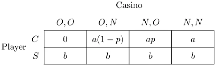
Proof. Figure 4 represents the player’s expected payoffs for each possible combination of the casino’s strate-gies.
Player
Casino
O, O O, N N, O N, N
C 0 a(1−p) ap a
S b b b b
Figure 4: The player’s expected payoffs
Based on the best response to the player’s action of each type of the casino, the only feasible equilibria from this table are [C,(O, N)] and [S,(N, N)]. The latter is not an equilibrium because we have assumed
that a > b; that is, if the casino does not observe in either state, the player prefers to count cards. The
former is an equilibrium if and only if
a(1−p)≥b,
which is equivalent to the requirement that
(4.1) p≤a−b
a .
Proposition. There exists a mixed strategy equilibrium in which the player chooses to count cards with probability
q=FL
a ,
the vigilant casino chooses to observe with probability
r=a−b
pa ,
and the non-vigilant casino always chooses not to observe. The existence of this equilibrium depends on the value ofp.
Proof. By setting the probability of card counting to be
q=FL
a ,
the player makes the vigilant casino indifferent between observing and not observing. Given this probability, the non-vigilant casino always chooses not to observe. The vigilant casino must then choose its mixed strategy such that the player is indifferent between choosing to count cards and choosing to employ a fixed strategy.
Let z be the probability that the vigilant casino assigns to observing. It must therefore choose z such that
This requires setting
z=a−b
pa .
In order to verify that this solution is in fact an equilibrium, it must be the case that
a−b
pa <1.
This condition is equivalent to the requirement that
p > a−b
a .
Therefore, when (4.1) holds, the unique equilibrium is in pure strategies and when (4.2) holds, the unique equilibrium is in mixed strategies.
4.3
The Casino’s Type and the Player’s Skill are Both Unknown
The discussion in subsection 4.2 assumes that if the player chooses to count cards and is not caught doing so, he receives a fixed payoff,a. In reality card counting is not a simple enterprise. A player’s success depends on his skill. We now allow the player to be of either high or low ability. The payoff to counting cards,a, can take on one of two values, such that the high skill player receives aH, the low skill player receivesaL, and
aL< b < aH. We continue to assume that the casino can be either vigilant or non-vigilant, that the player
does not know the casino’s type, and that both types of the player believe that the casino is vigilant with probability p. We also assume that the casino does not know whether the player is of high or low skill, but that both types of the casino believe that the player is of high skill with probabilityw. Let
(4.2) aL< FL< FH and
(4.3) FL< aH< FH.
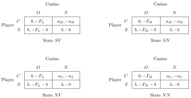
The game is represented in Figure 5, where each state is defined by the type of the player followed by the type of the casino.5
5We make the assumptions in (4.2) and (4.3) based on the following reasoning:
• if the player is not a skilled card counter (a=aL), the casino does not view his strategy as threatening and will not
exert effort to stop him; and
Player Casino O N C 0,−FL aH,−aH S b,−FL−b b,−b StateSV Player Casino O N C 0,−FH aH,−aH S b,−FH−b b,−b StateSN Player Casino O N C 0,−FL aL,−aL S b,−FL−b b,−b State N V Player Casino O N C 0,−FH aL,−aL S b,−FH−b b,−b StateN N
Figure 5: The casino does not know the player’s type and the player does not know the casino’s type.
Proposition. The unique pure-strategy equilibrium6 of this game is
[(C, S),(N, N)],
where the first ordered pair represents the actions of each type of the player (with the skilled player’s strategy first) and the second ordered pair represents the actions of each type of the casino (with the vigilant casino’s strategy first). The existence of this equilibrium depends on the value ofw.
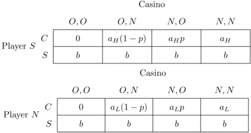
Proof. Figure 6 represents each type of player’s expected payoff to each strategy of the casino.
Based on the best response of each type of the casino to the player’s actions, the only possible equilibria are [C,(O, N)] and [S,(N, N)] for the skilled player and [C,(N, N)] and [S,(N, N)] for the unskilled player. In the former case, [S,(N, N)] is not possible because the skilled player will deviate. [C,(O, N)] is possible if and only if
(4.4) p≤ aH−b
aH
.
In the latter case, [C,(N, N)] is not possible because the unskilled player prefers not to count. [S,(N, N)] is possible regardless of the value ofp. However, given the difference between the best actions of the casino and the player in each state of the player’s skill, neither of these outcomes represent a pure strategy equilibrium.
Figure 7 represents each type of casino’s expected payoff to each strategy of the player.
6The reader will notice that the existence of a mixed-strategy equilibrium is also possible in this case; however, it is omitted
PlayerS Casino O, O O, N N, O N, N C 0 aH(1−p) aHp aH S b b b b PlayerN Casino O, O O, N N, O N, N C 0 aL(1−p) aLp aL S b b b b
Figure 6: The player’s expected payoffs to each strategy of the casino.
CasinoV Player C, C C, S S, C S, S O −FL −FL−b(1−w) −FL−wb −FL−b N −aHw−aL(1−w) −aHw−b(1−w) −bw−aL(1−w) −b CasinoN Player C, C C, S S, C S, S O −FH −FH−b(1 +w) −FH−bw −FH−b N −aHw−aL(1−w) −aHw−b(1−w) −bw−aL(1−w) −b
Figure 7: The casino’s expected payoffs to each strategy of the player.
Based on the best response of each type of the player to the casino’s actions, the only possible equilibria are [O,(S, S)] and [N,(C, S)] for both the vigilant and non-vigilant casino; but [O,(S, S)] is not possible because both types of casino have an incentive to change their strategy to N. [N,(C, S)] is an equilibrium in each case if and only if
w≤ Fi
aH
,
wherei=Lfor the vigilant casino andi=H otherwise. Thus when
w≤ FL
aH
<FH aH there exists a pure strategy equilibrium of the form
5
Computer Simulation
In the majority of the models used in this discussion, variables have been used to represent potential payoffs. From a theoretical standpoint, this is useful because it allows the games to be solved without knowing specific payoffs. Practically, though, the actual payoffs are necessary in order to apply the models to real life situations and decision-making.
One method for determining some of the more complex payoffs is to simulate the strategies using computer programming (specifically C++). After performing thousands of simulations of the different strategies, we can get estimates of the payoffs by using the law of large numbers. For example, we can use computer simulations to determine the expected payoff of a perfect card counter playing a game of Blackjack in which there are 3 decks. In this example, the player would follow the rules of card counting for betting and standard Blackjack strategy for hitting and staying. Of course, we do need to make some assumptions, such as the “low” bet amount and the “high” bet amount, but this issue is much more manageable.
As the number of simulations becomes large, observing the outcomes of this simulation will help give us an accurate picture of the payoffs for the strategy. One of the best reasons in favor of using this method to find payoffs is that it is completely adaptable to any situation. As we can see in real life, the number of decks used by the casino and the strategies utilized by the dealer can be quite diverse. Thus, we should have a very flexible (yet automated) method for determining payoffs in specific situations to give the model life.
Appendix B contains the code of a sample C++ program we created that shuffles one deck and runs a game of Blackjack (no doubles or splits, the dealer is forced to hit until 17, Blackjack pays 3-to-2) with the player using the ideal Blackjack strategy. The program displays the player’s cards, the dealer’s cards and the resulting payoff. The program can be iterated as many times as the user requires in order to obtain the expected payoff of the strategy.
In this sample, the program simulated 250,000 hands of Blackjack and displays the resulting expected value. This process can be further looped as many times as required: for example, we simulated 25 million hands of Blackjack with an expected value of−.0148011 dollars on $1 bets. Obviously the estimate improves when more simulations are run.
The sample program can be adapted with relative ease to model a card counter and calculate an expected payoff under many varying circumstances, including different numbers of decks, variations in rules, and expanded action spaces with splits and doubles.
6
Extensions
After laying a solid background in theory and basic modeling, we can see that there are multiple possibilities for extension of our work on the game of Blackjack. Two of the most prominent areas that pose additional questions are masking of signaling and absent-mindedness.
6.1
Signaling
We have shown in subsection 4.3 that the nature of the equilibrium in the card counting game depends on the probability with which the casino believes the player is skilled at counting cards. If the casino believes that this probability is sufficiently low, it will not observe the player, leaving the skilled player open to gain from counting cards. It is in the best interest of the player, if he is skilled, to send signals that cause the casino to perceive that he is either unskilled or not a card counter, and therefore choose not to observe him. These signals can take several forms. Generally, the wagering structure of a card counter’s strategy entails a series of small bets followed by very large ones when the count is favorable. Moreover, card counters are often identified by the large variation in their bets. In order to mask his type as a card counter the player may distort his wagering strategy in order to avoid drawing attention to himself.
Additionally, since card counters will inevitably send signals of their type, they can avoid drawing at-tention to themselves by working in teams. These teams are composed of players who track the count of a table and draw the attention of another player when the count is favorable. Dividing the tasks in this manner lessens the probability of detection by the casino, because the casino’s primary source of signaling information is eliminated.
6.2
Absent-Mindedness
Although card counting in theory is not incredibly complicated, actually keeping the correct count is rather difficult for most people, particularly in a casino environment that provides many distractions. We can certainly imagine a situation in which the player does not know his own ability, and thus does not know whether he is a skilled card counter or a mediocre card counter.
Furthermore, the success of a card counter hinges not only whether he correctly accounted for the cards currently on the table, but also on whether he correctly counted all hands prior to the current one. It is surely within reason to consider a situation in which a card counter does not recall the exact count prior to the dealing of cards in the current hand. In this situation, the “absent-minded” card counter faces a dilemma as to whether he should simply bet normally and restart the count, or whether he should use the
count he believes to be correct with a particular assigned probability.
7
Conclusion
As we have shown through the example ofSix, even a seemingly simple game can require a rather lengthy op-timal strategy. Despite the relative complexity of Blackjack when compared toSix, the same basic analytical tools of game theory can be used to determine the rational player’s optimal approach.
The introduction of card counting to optimize betting strategy adds a further layer of complication. In particular, the player then has to decide whether card counting or standard Blackjack strategy is optimal given additional considerations, including the casino’s potential attempts to be tough on card counters and the extent of both the player’s ability and memory.
While all of these additional extensions add complexity to the models and solutions, the use of game theory, statistical methods, and computer simulation can help provide optimal solutions and strategies for both the Blackjack players and the casinos encountering situations involving imperfect information.
References
[1] Baldwin, R, Cantey, W, Maisel, H, & McDermott, J. (1956). The Optimum strategy in Blackjack.
Journal of the American Statistical Association, 51(275), 429-439.
[2] Friscolanti, M. (2009). Don’t count on it. Review of the International Statistical Institute, 122(8), Re-trieved from http://web.ebscohost.com/.
[3] Manson, A. (1975). Optimum zero-memory strategy and exact probabilities for 4-deck Blackjack . The American Statistician , 29(2), 84-88.
[4] Osborne, M. (2004). An introduction to game theory. Oxford: New York.
[5] Patterson, J. (2002, July). Harvey Dubner: the forgotten man of Blackjack.Gambling Times, Retrieved from http://www.gamblingtimes.com/writers/jpatterson/jpatterson summer2002.htm.
[6] Sadun, E. (2009, February 19). Casino regulators issue alert over iphone card-counting app.ARS Tech-nica, Retrieved from http://arstechnica.com/apple/news/2009/02/casino-operators-issue-warning-over-iphone-card-counting-app.ars.
[7] Thomsen, D. (1975). Beating the game. Society for Science & the Public, 107. Retrieved from http://www.jstor.org/stable/3959663.
[8] Thorp, E. (1961). A favorable strategy for twenty-one.Proceedings of the National Academy of Sciences of the United States of America. Retrieved (2009, December 1) from http://www.jstor.org/stable/70615.
[9] Thorp, E. (1969). Optimal gambling systems for favorable games.Review of the International Statistical Institute, 37(3), Retrieved from http://www.jstor.org/stable/1402118.
[10] Blackjack tactics. (2006) Retrieved from http://www.Blackjacktactics.com/Blackjack/strategy/card-counting/hi-lo/.
A
Strategies in
Six
and Blackjack
Omitted Due to Space Considerations
Figure 8: All the possibilities and payoffs in a game ofSix. Even for such a simple game, the probability tree is enormous. (This figure is omitted here due to its size. Interested readers may inquire with the authors to receive it.) A: 4, B: 4 Hit 3 A: 7 bust, B: 4 (-x, x) 1 A: 5, B: 4 Hit 3 A: 5, B: 7 bust (2x, -2x) Stay (2x, -2x) Stay Hit 3 A: 4, B: 7 bust (2x, -2x) 1 A: 4, B: 5 (-x, x) Stay (0, 0)
Figure 9: A close-up on the probability tree of the game of Six. The strategy set given that both players haven= 4. Probability of drawing the three is 12, as is the probability of drawing the one.
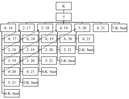
K 5 A: 16 A: 17 2: 18 3: 19 4: 20 5: 21 6-K: bust 2: 17 A: 18 2: 19 3: 20 4: 21 5-K: bust 3: 18 A: 19 2: 20 3: 21 4-K: bust 4: 19 A: 20 2: 21 3-K: bust 5: 20 A: 21 2-K: bust 6: 21 7-K: bust
Figure 10: An examination of the possibilities of a known hand in Blackjack. The arrows represent akin situations..
Figure 11: Thorp’s (1961) best strategy table for Q(5) = 0 (i.e., no more fives in the game).
B
C++ Code
The contents of this appendix have been omitted due to space considerations. The code is available from the authors upon request for those readers interested in examining it.