© 2001 Hirschmann Electronics GmbH & Co. KG
Manuals and software are protected by copyright. All rights reserved. The copying, reproduction, translation, conversion into any electronic medium or machine scannable form is not permitted, either in whole or in part. An exception is formed by the preparation of a backup copy of the soft-ware for your own use.
This manual has been created by Hirschmann electronics GmbH & Co. KG according to the best of our knowledge. Hirschmann reserves the right to change the contents of this manual without prior notice. Hirschmann can give no guarantee in respect of the correctness or accuracy of the details in this manual.
Hirschmann can accept no responsibility for damages, resulting from the use of the network components or the associated operating software. For the rest, we refer to the conditions of use specified in the license contract.
Printed in Germany
Hirschmann Electronics GmbH & Co. KG Automation and Network Solutions Stuttgarter Straße 45-51
Hirschmann worlwide:
U Germany
Hirschmann Electronics GmbH & Co. KG Automation and Network Solutions
Stuttgarter Straße 45-51 D-72654 Neckartenzlingen Tel. ++49-7127-14-1527 Fax ++49-7127-14-1542
email: [email protected] Internet: www.hirschmann.de
U Austria
Hirschmann Austria GmbH Oberer Paspelweg 6-8 A-6830 Rankweil-Brederis Tel. ++43-5522-3070 Fax ++43-5522-307555 A-1230 Wien
Tel. ++43-1-6174646 Fax ++43-1-6174646
email: [email protected]
U Switzerland
Hirschmann Electronics GmbH & Co. KG, Neckartenzlingen Niederlassung Uster
Seestr. 16 CH-8610 Uster
Tel. ++41-1905-8282 Fax ++41-1905-8289
U France
Hirschmann Electronics S.A. 24, rue du Fer à Cheval, Z.I. F-95200 Sarcelles
Tel. ++33-1-39330280 Fax ++33-1-39905968 email: [email protected]
U Great Britain
Hirschmann Electronics Ltd. St. Martins Way
St. Martins Business Centre GB-Bedford MK42 OLF Tel. ++44-1234-345999 Fax ++44-1234-352222
email: [email protected]
U Netherlands
Hirschmann Electronics B.V. Pampuslaan 170
NL-1382 JS Weesp Tel. ++31-294-462555 Fax ++31-294-480639 email: [email protected]
U Spain
Hirschmann Electronics S.A. Calle Traspaderne, 29
Barrio del Aeropuerto Edificio Barajas 1,2 Planta E-28042 Madrid
Tel. ++34-1-7461730 Fax ++34-1-7461735
U Hungary
Hirschmann Electronics Kft. Rokolya u. 1-13
H-1131 Budapest Tel. ++36-1-3494199 Fax. ++36-1-3298453
email: [email protected]
U USA
Hirschmann Electronics Inc.
30 Hook Mountain Road _ Unit 201 USA-Pine Brook, N. J. 07058
Tel. ++1-973-8301470 Fax ++1-973-8302000
email: [email protected]
U Singapore
Hirschmann Electronics Pte. Ltd. 3 Toh Tuck Link
# 04-01 German Districentre Singapore 596228
Tel: (65)463 5855 Fax:(65) 463 5755
email: [email protected]
U China (PRC)
Hirschmann Electronics Shanghai Rep. Office
Room 518, No. 109 Yangdang Road Lu Wan District, 200020
SHANGHAI, PRC
Tel +86-21 63 58 51 19 Fax +86-21 63 58 51 25
Content
1 Overview
151.1 Historical Development of Ethernet 17
1.2 The ISO/IEC 8802-3 Standard 21
1.2.1 CSMA/CD Access Method 21
1.2.2 Collisions 23
1.2.3 Interpacket Gap 28
1.2.4 Full duplex 29
1.3 Frame structure 31
1.4 IP address 35
1.4.1 Network mask 36
2 Network Planning
412.1 Planning Rules 43
2.1.1 Planning Guidelines for 10 MBit/s Ethernet 43 2.1.2 Planning Guidelines for 100 MBit/s Ethernet 47 2.1.3 Planning Guidelines for 100 MBit/s Ethernet 48
2.2 Maximum Network Size 49
2.2.1 Hub Networks 49
2.2.2 Switch networks 58
2.3 Variability 59
2.4 Redundancy 65
2.4.1 Normal mode ('as-delivered' setting) 65
2.4.2 Frame redundancy (10 Mbit/s Ethernet) 65
3 Network management
713.1 Management principles 73
3.2 Statistic tables 77
3.3 Security 79
3.3.1 SNMP 79
3.3.2 SNMP traps 80
4 Switching Functions
814.1 Frame switching 83
4.1.1 Store and Forward 83
4.1.2 Multi-address capability 83
4.1.3 Learning addresses 83
4.1.4 Prioritization 84
4.1.5 Tagging 84
5 Spanning tree algorithm
895.1 Tasks 91
5.2 Rule for creating the tree structure 93
5.2.1 Bridge identification 93
5.2.2 Root path costs 94
5.2.3 Port identification 95
6 Management Information Base
MIB
1016.1 MIB II 105
6.1.1 System Group (1.3.6.1.2.1.1) 105
6.1.2 Interface Group (1.3.6.1.2.1.2) 108
6.1.3 Address Translation Group (1.3.6.1.2.1.3) 109
6.1.4 Internet Protocol Group (1.3.6.1.2.1.4) 109
6.1.5 ICMP Group (1.3.6.1.2.1.5) 111
6.1.6 Transfer Control Protocol Group (1.3.6.1.2.1.6) 112 6.1.7 User Datagram Protocol Group (1.3.6.1.2.1.7) 113 6.1.8 Exterior Gateway Protocol Group (1.3.6.1.2.1.8) 113 6.1.9 Simple Network Management Protocol Group
(1.3.6.1.2.1.11) 114
6.1.10RMON-Gruppe (1.3.6.1.2.1.16) 115
6.1.11dot1dBridge (1.3.6.1.2.1.17) 117
6.1.12MAU Management Group (1.3.6.1.2.1.26) 122
6.2 Private MIB 125
6.2.1 Device Group 125
A Appendix
131FAQ 133
Literature references 135
Reader’s comments 137
1 Overview
This chapter allows to overview the historical development of Ethernet and his important charactaristics.
1.1 Historical Development of
Ethernet
The constant growth in the use of data processing systems and their intro-duction into many areas (office communications, scientific-technical applica-tions, construction, manufacturing, etc.) make capacity and
high-function data networks mandatory. One possible way to economically solve this problem is the use of local area networks.
In 1972 Xerox began to develop the bus-connected local area network (LAN) at its Palo Alto Research Center using the CSMA/CD access method. The name of the access method stands for three actions that characterize it::
D Carrier Sense D Multiple Access D Collision Detection.
The increasing significance of LANs caused three companies, Digital Equip-ment Corporation (DEC), Intel Corporation, and Xerox, to found the DIX consortium, whose goal was to continue development, building on the good results already achieved by Xerox.
In 1980, DIX published the first specifications for Ethernet Version 1.0. At the same time, working group 802 of the Institution of Electronical and Electronic Engineers (IEEE) began to develop a standard for a CSMA/CD bus LAN. The Ethernet Version 1.0 specifications formed the base for this work. The T24 Committee on Communication Protocols of the European
Computer Manufacturers Association (ECMA) also provided useful input for
the development of the standard.
The result of this work is IEEE recommendation 802.3. In 1982, the DIX group modified their Ethernet Version 2.0 specifications to conform with the IEEE recommendations. In 1985, the recommendation was raised to the sta-tus of a standard.
The standard was submitted to the International Standardization Organizati-on / InternatiOrganizati-onal Electrotechnical CommissiOrganizati-on (ISO / IEC) with the goal of creating an international standard. This resulted in its being published as the ISO/IEC 8802-3 International Norm in 1988. No significant technical changes were made to the original standard as a result of this.
A further significant step for the success of local area networks was the crea-tion of the ISO/OSI reference model (Internacrea-tional Standardizacrea-tion Organisa-tion / Open System InterconnecOrganisa-tion).
This reference model had the following goals:
D To define a standard for information exchange between open systems;
D To provide a common basis for developing additional standards for open systems;
D To provide international teams of experts with functional framework as the basis for independent development of every layer of the model;
D To include in the model developing or already existing protocols for com-munications between heterogeneous systems;
D To leave sufficient room and flexibility for the inclusion of future develop-ments.
The reference model consists of 7 layers, ranging from the application layer to the physical layer.
The model was published in October 1984 in international standard ISO 7498.
Fig. 1: OSI reference model
However, the data rate and the transmission media were permanently adap-ted. The next data rate - 100 Mbit - was actually already attained by FDDI. The transition from 10 MBit Ethernet to FDDI was, however, not a very smooth one for users. Standardization of FDDI was also very sluggish, and the data terminal equipment never fell to price level that might have made them competitive in the market.
Thus, the development of 100 MBit Ethernet began. On the physical level, FDDI components were adopted. Since 1994 FDDI has at times been im-plemented with TP cable. Initially there were two approaches to finding a solution. The first one, Fast Ethernet, simply adapted all transmission parameters to the new speed. The other approach defined a new access method - demand priority - and from that time on was referred to as project group 802.12 by the IEEE. The sole disadvantage of the first proposal -reducing the spatial extent of a network to one tenth of its size - became insignificant due to the widespread availability of bridges and switches. Consequently, it became the new standard. It was adopted in 1995. Although 802.12 was also adopted, it hardly plays a role anymore.
Application
Presentation
Session
Transport
Network
Data-Link
Physical
7 6 5 4 3 2 1Access to communication services from an application program
Definition of the syntax for data communication
Set up and breakdown of connections by synchronization and organization of the dialog
Specification of the terminal connection, with the necessary transport quality
Transparent data exchange between two transport entities
Access to physical media and detection and resolution of transmission errors
The next level of speed appeared once and for all to belong to another form of transmission - ATM - which promised data rates in excess of 622 MBit. This is why the idea of 1 GBit Ethernet, presented in 1995, was not taken very seriously. As it turned out, this appeared to be a quite premature. Work on the standard proceeded very quickly. For example, it was possible to adopt transmission components from Fiberchannel. Products already became available far before the standard was adopted in 1998. The first chips ap-peared at the end of 1996, and functional devices hit the market a year later. In 1999 even twisted pair transmission was standardized at this speed. Ever since Gigabit Ethernet has become commonplace and the digitalization has continued its torrid pace, calls for even more bandwidth have become increasing louder. This has led to work on developing a 10 Gigabit Ethernet standard that got underway in 1999.
1.2 The ISO/IEC 8802-3 Standard
The most significant characteristic of a local area network conforming to ISO/ IEC 8802-3 is that all network users have equal access to the transmission medium. In order to handle the inevitable collisions, reliable collision detec-tion and unambiguous resoludetec-tion are mandatory elements of any implemen-tation of this norm.
1.2.1 CSMA/CD Access Method
There is no central station to monitor or control access to the local area net-work. Each member of the network monitors traffic on the network and, if the network is free, can start transmitting data immediately.
Sequence of a transmission occurrence:
Carrier Sense: Network members check to see if the transmission medi-um is free.
Multiple Access: If the transmission medium is free, any network member can start transmitting data.
Collision Detection: If more than one member of the network start trans-mitting data simultaneously, a data collision will result. The transtrans-mitting members will detect the collision and terminate transmission. A backoff strategy determines when the members can retry the data transmissions.
1
2
3
Fig. 2: CSMA/CD Access
Transmission medium available? no
yes Network access
Terminate network access Network member ready to transmit
Start to transmit data
Collision?
no
yes
End of transmission? no
yes
Wait as determined by backoff strategy
Transmit jam signal
1.2.2 Collisions
The logical result of the CSMA/CD method is that there is a finite probability that multiple users could attempt to access the medium simultaneously. For that reason, the access method must have a mechanism for dealing with any collisions as they occur.
Requirements for this mechanism:
D Detection of each collision by the participating network members.
D Termination of the transmission attempt in case of a collision.
D Renewed transmission attempt if the previous attempt has failed due to a collision.
The following conventions have been agreed to for meeting these requi-rements:
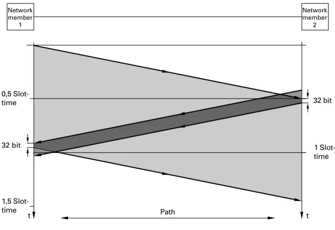
The signal transmission time depends on the minimum data packet length. ISO/IEC 8802-3 defines the time window (slot time) to be the time it takes from the beginning of the transmission until a collision at the far end of the transmission medium occurs. The slot time is 51.2 µs.
The minimum data packet length is equal to the slot time. This insures that the transmitting station can detect a collision while the transmission is still taking place and therefore knows that the transmission has failed.
“Collision detection as a function of time and location. The jam (collision notification) signal from member 2 reaches member 1 while member 1 is
still sending.” on page 24 shows this relationship. Network member 1
starts to transmit. Just before the transmission reaches network member 2, member 2 also begins to transmit. The signal from member 1 then rea-ches member 2 who detects the collision and transmits the 32-bit jam signal before terminating its own transmission. The jam signal arrives at member 1 within the slot time interval, that is, while member 1 is still transmitting. Member 1 is thus also able to detect the collision.
Fig. 3: Collision detection as a function of time and location.
The jam (collision notification) signal from member 2 reaches member 1 while member 1 is still sending.
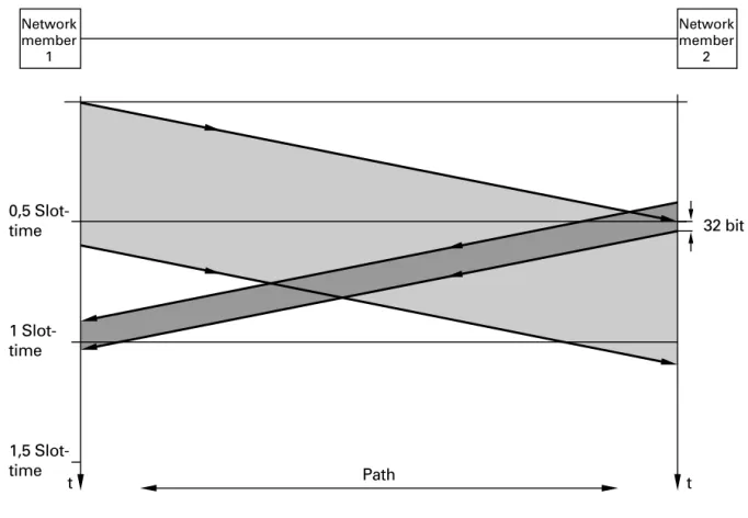
If a data packet is shorter than the slot time, it is possible that a transmit-ting member of the network might not be able to detect that a data packet it had just sent has been damaged by a collision. In that case, there would be no re-transmission of the damaged packet (see Fig. 4).
Path 1,5
Slot-time
1 Slot-time 32 bit 0,5
Slot-time
t t
32 bit
Network member
1
Network member
Fig. 4: Data packet too short.
Network member 1 is not able to detect that the data packet just sent has been damaged by a collision.
ISO/IEC specifies a slot time of 51.2 µs. Taking into consideration the repeater propagation times of a network of maximum size, this results in a maximum network size of 2500 meters. “Network Planning” on page 41
describes how this maximum can be extended.
Path 1,5
Slot-time 1 Slot-time
32 bit 0,5
Slot-time
t t
Network member
1
Network member
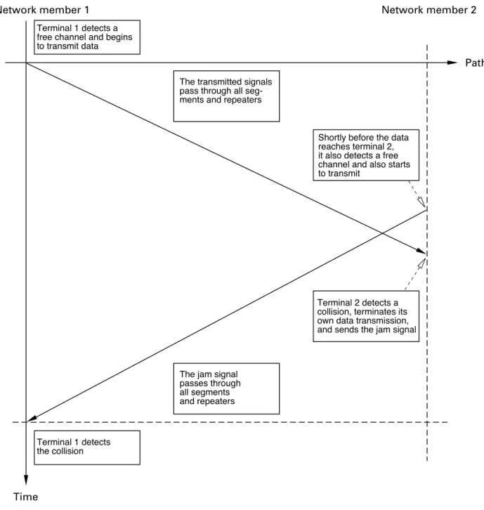
Fig. 5: Collision detection model
If a transmitting network station detects a collision, it must send at least 32 more bits (jam size) before finally terminating its transmission attempt. This minimum collision duration of 3.2 µs insures that each station in the network detects the collision.
Terminal 1 detects a free channel and begins to transmit data
Terminal 1 detects the collision
The transmitted signals pass through all seg-ments and repeaters
Shortly before the data reaches terminal 2, it also detects a free channel and also starts to transmit
The jam signal passes through all segments and repeaters
Terminal 2 detects a collision, terminates its own data transmission, and sends the jam signal
Time
Network member 1 Network member 2
Path
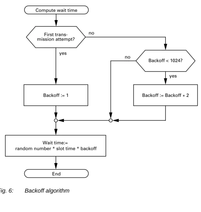
If a station in the network is unable to transmit its data packet completely due to a collision, then it must wait a predetermined length of time and re-attempt the transmission.
Fig. 6: Backoff algorithm
ISO/IEC 8802-3 allows up to 16 transmission attempts before finally giving up trying to send a data packet. The maximum value that "backoff" can as-sume is 1024. This means that "backoff" will not be increased after the tenth attempt.
3
yes Compute wait time
Wait time:=
random number * slot time * backoff
Backoff < 1024? no
no yes
Backoff := Backoff * 2 First
trans-mission attempt?
Backoff := 1
1.2.3 Interpacket Gap
A minimum gap between packets is required as recovery time for CSMA/CD sub-layers and the physical medium. ISO/IEC 8802-3 defines this minimum interpacket gap to be 9.6 µs.
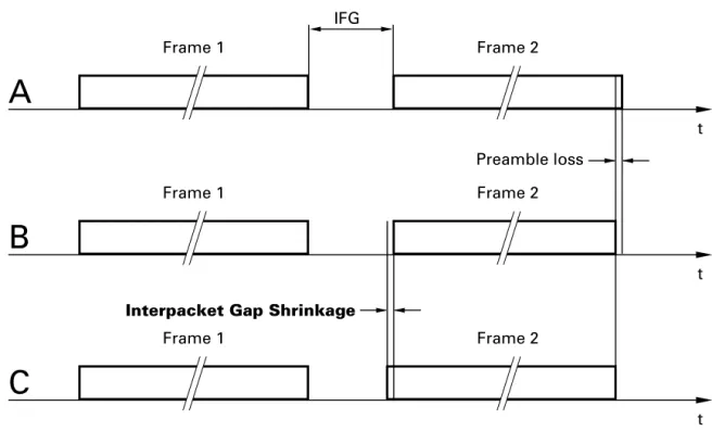
The varying bit loss (preamble loss) of two successive data packets on the same path can cause the interpacket gap to shrink. A repeater regenerates the lost preamble bits of any packet passing through it. This gap shrinkage is called interpacket gap shrinkage.
If the first data packet (frame) loses more preamble bits on reception than the subsequent packet - A and B(see Fig. 7), then the gap will be reduced after the preamble has been regenerated by the repeater - C(see Fig. 7).
Transmission rate Interpacket gap 10 MBit/s 9,6 µs
100 MBit/s 960 ns 1000 MBit/s 96 ns
Fig. 7: Schematic representation of Interpacket Gap Shrinkage
1.2.4 Full duplex
In half duplex operation, the port of the switch is connected to an Ethernet. All rules prescribed by the CSMA/CD access method must be followed. For example, it is not possible to send and receive data at the same time, and, in order to be sure of detecting collisions, the propagation time is limited. These restrictions are removed for full duplex operation. Instead of the well known bus structure, a point-to-point or bridge-to-bridge connection is used. Transmitting and receiving are conducted over two separate lines so that CSMA/CD rules can be ignored. Transmitting and receiving can take place at the same time at a particular port, which means that twice the bandwidth is available. By eliminating collisions it is possible to increase the effective data throughput by a factor of almost 10. The effective maximum through-put
t IFG
Frame 1 Frame 2
t
Frame 1 Frame 2
Preamble loss
t
Frame 1 Frame 2
Interpacket Gap Shrinkage
B
A
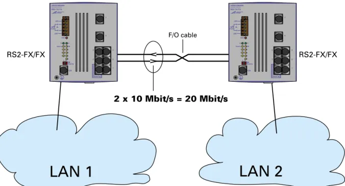
for Ethernet is 2 to 3 Mbit/s. Full duplex provides a bandwidth of 2 * 10 Mbit/s = 20 Mbit/s. The propagation time limitations needed for
collision detection no longer apply. This makes it possible to extend networks to much greater distances than are possible with ordinary Ethernet connec-tions.
Certain PC controller cards, such as that of Compaq and IBM, also supports this full duplex function, so that the 20 Mbit/s bandwidth can be achieved in a direct connection between these devices and a switch.
Abb. 8: Full duplex connection of two LANs
LAN 1
LAN 2
RS2-FX/FX RS2-FX/FX
F/O cable
2 x 10 Mbit/s = 20 Mbit/s
6 1 5 4 3 2 i RS2-TX/TX 7 1 0 +24V +24V* Fault FAULT P2 Stand by P1 RM 7 6 5 4 3 2 2 V.24 Stand by RM Stand by 6 1 5 4 3 2 i RS2-TX/TX 7 1 0 +24V +24V* Fault FAULT P2 Stand by P1 RM 7 6 5 4 3 2 2 V.24 Stand by RM Stand by
1.3 Frame structure
Within the scope of the CSMA/CD access principle, data frames specified in ISO/IEC 8802-3 are used for data transfer.
A frame is a data packet with a defined form and length that consists of si-gnals in Manchester code. A frame is transferred serially with a data rate of 10 Mbit/second, whereby the individual bits are combined in octets (bytes of 8 bits each). All octets of one frame, with the exception of the Frame Check Sequence Field (FCS), are transferred with the least significant bit (LSB) first.
Fig. 9: Data transfer direction
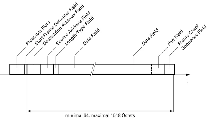
A frame has a minimum length of 64 octets and a maximum of 1518
(see Fig. 10). The length of the frame is calculated without a preamble and
the Start Frame Delimiter (SFD).
A frame consists of:
LSB MSB
Time Octet
U Preamble Field
The preamble, consisting of a string of alternate ones and zeros, serves to stabilize and synchronize the respective recipient to the incoming frame.
Length: 7 octets (10101010...10101010)
U Start Frame Delimiter Field
(SFD Field)
The SFD marks the start of the destination address (Destination Address Field).
Length: 1 octet (10101011)
U Destination Address Field
Contains the frame's destination address. Length: 6 octets (48 bits)
U Source Address Field
Contains the frame's source address. Length: 6 octets (48 bits)
U Length/Type Field
The ISO/IEC 8802-3 standard uses this field as the length field to specify the number of octets in the subsequent data field that are to be transfer-red (values between 0 and 1518).
Ethernet Version 2.0 specifies this field as the type field, which contains parameters specific to the manufacturer (values > 1518).
U Data- und Pad Field
The user data is transferred in the data field. Lengthmin:46 octets(368 bits)
max: 1500 octets(12 000 bits)
A data field that is less than 46 octets is filled up by a pad field containing additional octets.
U Frame Check Sequence Field (FCS Field)
A check value is calculated on the basis of the contents of the previous fields (without the preamble and SFD) and is written into the FCS field. On the receiving end, a check value is also calculated on the basis of the same principle. This value agrees with the one in the FCS field if the data was transferred without errors occurring.
Length: 4 octets (32 bits)
Fig. 10: Frame structure
t
minimal 64, maximal 1518 Octets
Preamble FieldStart Frame Delimiter FieldDestination Address FieldSource Address FieldLength/Type FieldData Field Data Field Pad FieldFrame Check
1.4 IP address
The IP address consists of 4 bytes. These 4 bytes are written in decimal no-tation, each separated by a dot.
Since 1992, five classes of IP addresses have been defined in RFC 1340. The most frequently used address classes are A, B and C.
The network address represents the permanent part of the IP address. It is as-signed by the DoD (Department of Defense) Network Information Center.
Fig. 11: Bit notation of the IP address
All IP addresses belong to class A when their first bit is a zero, i.e. the first decimal number is less than 128.
The IP address belongs to class B if the first bit is a one and the second bit is a zero, i.e. the first decimal number is between 128 and 191.
The IP address belongs to class C if the first two bits are a one, i.e. the first decimal number is higher than 191.
Assigning the host address (host id) is the responsibility of the network operator. He alone is responsible for the uniqueness of the IP addresses he assigns.
Class network address Host address
A 1 Byte 3 Bytes
B 2 Bytes 2 Bytes
C 3 Bytes 1 Byte
Table 2: IP address classification
Network address Host address
1.4.1 Network mask
Routers and gateways subdivide large networks into subnetworks. The net-work mask assigns the individual devices to particular subnetnet-works.
The subdivision of the network into subnetworks is performed in much the same way as IP addresses are divided into classes A to C (network id). The bits of the host address (host id) that are to be shown by the mask are set to one. The other host address bits are set to zero in the network mask (see following example).
Example of a network mask:
255.255.192.0 Decimal notation
11111111.11111111.11000000.00000000 Binary notation
Subnetwork mask bits Class B
Example of IP addresses with subnetwork allocation in accordance with the network mask from the above example:
1.4.2 Example of how the network mask is used
In a large network it is possible that gateways and routers separate the ma-nagement agent from its mama-nagement station. How does addressing work in such a case?
129.218.65.17 Decimal notation
10000001.11011010.01000001.00010001 binary notation
128 < 129 ≤ 191 ➝ Class B
Subnetwork 1 Network address
129.218.129.17 Decimal notation
10000001.11011010.10000001.00010001 binary notation
128 < 129 ≤ 191 ➝ Class B
Subnetwork 2 Network address
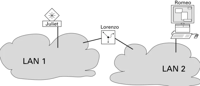
Fig. 12: Management agent that is separated from its management station by a router
The management station ”Romeo” wants to send data to the management agent ”Juliet”. Romeo knows Juliet's IP address and also knows that the rou-ter ”Lorenzo” knows the way to Juliet.
Romeo therefore puts his message in an envelope and writes Juliet's IP address on the outside as the destination address. For the source address, he writes his own IP address on the envelope.
Romeo then places this envelope in a second one with Lorenzo’s MAC address as the destination and his own MAC address as the source. This process is comparable to going from Layer 3 to Layer 2 of the ISO/OSI base reference model.
Finally, Romeo puts the entire data packet into the mailbox. This is compa-rable to going from Layer 2 to Layer 1, i.e. to sending the data packet via the Ethernet.
Lorenzo receives the letter and removes the outer envelope. From the inner envelope he recognizes that the letter is meant for Juliet. He places the inner envelope in a new outer envelope and searches his address list (the ARP ta--ble) for Juliet’s MAC address. He writes her MAC address on the outer enve-lope as the destination address and his own MAC address as the source address. He then places the entire data packet into the mail box.
Romeo
LAN 1
Lorenzo
LAN 2
Juliet receives the letter and removes the outer envelope, exposing the inner envelope with Romeo’s IP address. Opening the letter and reading its con--tents corresponds to transferring the message to the higher protocol layers of the ISO/OSI layer model.
Juliet would now like to send a reply to Romeo. She places her reply in an envelope with Romeo’s IP address as destination and her own IP address as source. The question then arises, where should she send the letter, since she did not receive Romeo’s MAC address. It was lost when Lorenzo replaced the outer envelope.
By comparing her IP address to Romeo's with the aid of the network mask, Juliet would immediately recognize that Romeo lives nowhere close by, and that to call out the window would be pointless.
In the MIB, Juliet finds Lorenzo listed under the variable
hmNetGate-wayIPAddr as a means of communicating with Romeo. The envelope with
the IP addresses is therefore placed in a further envelope with the MAC de-stination address of Lorenzo.
The letter then travels back to Romeo via Lorenzo the same way the first let-ter traveled from Romeo to Juliet.
2 Network Planning
The collision mechanism of an ISO/IEC 8802-3 LAN makes it necessary to limit signal delay value (see“The ISO/IEC 8802-3 Standard” on page 21). As a consequence, the physical size of the network is also limited. The signal delay value limitation means that the distance between any two stations in the network cannot exceed 4520 meters. ISO/IEC 8802-3 allows a maximum distance of only 2500 meters, however. This reduction is due to the delays introduced by the transmission components, primarily the repeaters.
The path variability value (see“Variability” on page 59) is just as important for correct network functioning as signal delay value. Until now, it was neces-sary to limit the number of repeaters to four in order to guarantee a minimum interpacket gap size. The limitation of four repeaters was dropped from the standard with the publication of Chapter 13 of ISO/IEC 8802-3. Instead of li-miting the number of repeaters in a network, Chapter 13 specifies the maxi-mum amount by which the interpacket gap can shrink and how this amount can be calculated for a particular signal path.
If a network requires more repeaters, Hirschmann repeaters are available that help you overcome this barrier. When passing through the repeater, the distance between packets shrinks by a smaller amount than permitted by the standard (see “Variability” on page 59).
2.1 Planning Rules
2.1.1 Planning Guidelines for 10 MBit/s Ethernet
When CSMA/CD networks were first being standardized, ISO/IEC 8802-3 li-mited itself to specifying standards that used the thick yellow coaxial cable (10BASE5 or yellow cable) as a transmission medium. The characteristics of this cable allow a maximum segment length of 500 meters.
Individual network stations are connected to the cable by transceivers. A ma-ximum of 100 transceivers with a minimum spacing of 2.5 meters can be con-nected to a segment. A transceiver cable (AUI cable) with a maximum length of 50 meters connects the network station to the transceiver.
Fig. 13: Ethernet base segment as specified in ISO/IEC 8802-3
In order to expand the network, the norm prescribes the use of repeaters for coupling two segments together.
DTE
Transceiver 10BASE5 (max. 500 m) Transceiver cable
max. 50 m Terminator
Fig. 14: Two basic Ethernet segments linked with repeaters
The delay value through a repeater is approximately the same as the delay value through a 500 meter coax segment.
This means that a signal path can contain a maximum of four repeaters and
five coax segments. Of the five coax segments, at least two must be pure
connecting segments (link segments) to which no stations are attached.
DTE
Transceiver cable
max. 50 m Terminator
Transceiver 10BASE5 (max. 500 m)
R
Fig. 15: Maximum signal path with repeaters
Because the thick yellow coax cable was too costly and too difficult to handle, the standard was extended to include the RG 58 coax cable. This was named the Cheapernet or thin wire Ethernet (10BASE2).
DTE Transceiver
Transceiver cable
max. 50 m Terminator
Repeater Link Segment
R
R
R
With a few restrictions and changes, the general specifications for the old standard were also applied to the newer standard. The trans-mission quality of this cable allows a maximum segment length of only 185 meters. Also, each segment can have a maximum of only 30 transceivers attached with a minimum spacing of 0.5 meters.
It is possible to mix standard Ethernet and Cheapernet in a single configura-tion.
Fig. 16: Cheapernet base segment
The increased popularity of this LAN type led to user requirements for more flexible connection capabilities:
D thinner cable diameters
D lower cost cable
D use of already installed telephone wiring
D use of already installed IBM Type 1 cabling
D better transmission characteristics
D better interception security
D reduction of the problems due to potential differences
D greater distance
D resistance to electromagnetic interference
The standards bodies met these demands by extending the standard to 10BASE-T for twisted pair cables and 10BASE-F for fiber optic cables. In contrast to the bus connection provided by 10BASE5 and 10BASE2, these two new cable types are able to offer pure point-to-point connections.
DTE
Transceiver 10BASE2 (max. 185 m) Transceiver cable
max. 50 m Terminator
With the standards as a framework, Hirschmann developed its network con-cept based on star distribution points, namely the active star couplers. Inter-face cards which can be plugged into the star couplers are available for all different transmission media, thus making it possible to operate a mixed net-work. The right medium is available for every requirement.
2.1.2 Planning Guidelines for 100 MBit/s Ethernet
Using half duplex segments the propagation delay between the terminal equipments is 512 bit times (BT) maximum. Add all components of the signal path plus a safety margin.
Characteristic 10BASE2 10BASE5 10BASE-F 10BASE-T Maximum cable length 185 m 500 m 2000 m 100m
Termination 50O 50O – 100O
Maximum transceivers 30 50 2 2
Minimum transceiver spacing 0,5 m 2,5 m – – Signal velocity 0,65 * c 77 * c 66 * c 59 * c
Table 3: The most important parameters for the media allowed by ISO/IEC 8802-3
Components Delay
RT2-TX/FX 84 BT
Class II Repeater 92 BT Terminal equipment with TP connection 50 BT Terminal equipment with F/O connection 50 BT Kat. 5 TP cable 1,112 BT/m
F/O cable 1 BT
Savety margin 4 BT Table 4: Signal delay in the sgnal path
2.1.3 Planning Guidelines for 100 MBit/s Ethernet
Using 1000 Mbit/s Ethernet generally the terminals are connected with Swit-ches directly. Thus the values in Table 5, “Length area in dependency of F/
O at 850 nm,” on page 48 and Table 6, “Length area in dependency of F/O
at 1300 nm,” on page 48 apply.
F/O type bandwith lengthproduct minimumdistance maximumdistance 62,5 nm multimode F/O 160 MHz * km 2 m 220 m 62,5 nm multimode F/O 200 MHz * km 2 m 275 m 50 nm multimode F/O 400 MHz * km 2 m 500 m 50 nm multimode F/O 500 MHz * km 2 m 550 m Table 5: Length area in dependency of F/O at 850 nm
F/O type bandwith length product
minimum distance
maximum distance 62,5 nm multimode F/O 500 MHz * km 2 m 550 m 50 nm multimode F/O 400 MHz * km 2 m 550 m 50 nm multimode F/O 500 MHz * km 2 m 550 m 10 nm singlemode F/O – 2 m 5000 m Table 6: Length area in dependency of F/O at 1300 nm
2.2 Maximum Network Size
2.2.1 Hub Networks
Chapter 13 of ISO/IEC 8802-3 describes the system requirements for a local area network that uses mixed transmission media. The standard assumes, however, that the communications components used exploit the tolerances that they are allowed.
The model 1 transmission system of Chapter 13 conforms basically with the currently valid configuration guidelines and only extends them with regard to the media that can be used. This model is un-suitable, however, if one wants to test the maximum limits of what is possible. For such a case, Model 2 pro-vides a much more precise description of how to calculate the maximum net-work range.
Model 2 takes the delay values of all the network components in the signal path into consideration. Considering all delay values is a very complex task, so Model 2 uses a simplification and defines fixed delay values for the indivi-dual segments. The disadvantage of this simplification is the invariance of the delay values for the various segments.
The following model for calculating the maximum network range is derived from Model 2. It has been optimally tailored to calculate a LAN made up of Hirschmann network components. Just like Model 2, it includes all network components found in the signal path. Only the form of the simplification has been changed, which leads to a much more precise calculation of maximum network range.
The basis for calculating the maximum network range is the maximum allo-wable signal delay value in the signal path between any two network stations. The critical case most frequently encountered can be found in the following situation (see Fig. 17).
Station 1 transmits data to station 2, which is quite close. The data is then sent into the rest of the network. Just before the data reaches station 3, sta-tion 3 starts to send data to stasta-tion 1 (cf. Appendix B, System Guidelines, B1.1 IEEE Std. 802.3-1985 Baseband Systems). Because station 3 must be sure to detect the data collision, the maxi-mum distance between stations 1 and 3 is 4520 meters given the standard minimum packet length and delay value through an ideal transmission link (fiber optic only).
Fig. 17: Critical case for maximum network range
Signal delays in the individual components of the signal path form a signifi-cant part of the total signal delay value. The delay value for a component is a simple way to determine the effect the delay value through the component has on the maximum range of the network.
Definition of "Propagation Equivalent":
The propagation equivalent describes the signal delay of a component loca-ted in the signal path. The signal delay is specified in terms of distance (me-ters) rather than time (seconds). The specifi-cation in meters indicates the distance that the signal could have traveled in the same time if it had been moving through a cable instead of the component.
Note: The conversion from time units to distance units assumes a cable
pro-pagation delay of 5 ns/m. A UTP cable has a signal delay of 5.6 ns/m(See “The most important parameters for the media allowed by ISO/IEC 8802-3”
on page 47.)
Ideal transmission link
Network station 3 Network
station 1
min. distance Network
station 2
V In order to determine if you comply with the standard, calculate the signal propagation time between the two members of the network that are farthest apart from one another.
Add up the values for all of the components within the signal path. The table onpage 47 lists all of the components belonging to the Hirschmann network concept. Signal delay for each component is specified in terms of the "propagation equivalent".
This total plus the length of the cable in the signal path must not exceed 4520 meters. In order to correctly compensate for the slower propagation velocity in UTP cable segments, you should add 10% to the length of tho-se cables..
n1 * Ü1 + ... + nx–1 *Üx–1 + nx *Üx + Σl ≤ 4520 m
nx = Number of ports in the signal path of the transmission components with the index x
Üx = propagation equivalent of a transmission component with the index x
Example 1:
The figure (see Fig. 18)shows a local area network that consists of twisted pair segments.
Seven Rail Hubs RH1-TP/FL lie in the signal path between the two network stations shown in the figure.
Fig. 18: Example of a reduced network range
UTP
= DTE = Rail Hub RH1-TP/FL
UTP
UTP F/O
F/O
UTP UTP
UTP
= Connection to TP port = Transceiver
DTE 1
DTE 2
The propagation equivalent for the interface cards and transceivers is calcu-lated as follows:
The total number of cable segment lengths may amount to 4520 m – 2020 m = 2500 m.
DTE 1
Transceiver Mini-UTDE 140 m Rail Hub 1 TP
TP
95 m 95 m Rail Hub 2 TP
TP
95 m 95 m Rail Hub 3 TP
TP
95 m 95 m Rail Hub 4 TP/FL
TP/FL
180 m 180 m Rail Hub 5 FL
FL
130 m 130 m Rail Hub 6 TP/FL
TP/FL
180 m 180 m Rail Hub 7 TP
TP
95 m 95 m Transceiver Mini-UTDE 140 m DTE 2
Example 2:
The figure (see Fig. 19) shows a LAN whose coax segments are connected together by fiber optic cables and star couplers. There are 5 star couplers equipped with 2 KYDE-S µC coax interface cards and 8 OYDE-S µC optical interface cards located between the network stations.
Fig. 19: Coax segments connected with fiber optic segments
fiber-optic
fiber-optic
fiber-optic
fiber-optic
= terminator
= star coupler = DTE
= coax transceiver = connection to OYDE
coax
= connection to KYDE-S µC
coax
The propagation equivalent for the interface cards and transceivers is calcu-lated as follows:
The total of the cable segment lengths may amount to 4520 m – 830 m = 3690 m.
DTE 1
Transceiver KTDE-S 205 m Star coupler 1 KYDE-S µC
OYDE-S µC
50 m 40 m Star coupler 2 OYDE-S µC
OYDE-S µC
40 m 40 m Star coupler 3 OYDE-S µC
OYDE-S µC
40 m 40 m Star coupler 4 OYDE-S µC
OYDE-S µC
40 m 40 m Star coupler 5 OYDE-S µC
KYDE-S µC
40 m 50 m Transceiver KTDE-S 205 m DTE 2
Example 3:
The figure (see Fig. 20)shows a mixed LAN consisting of coax, fiber optic and twisted pair segments. Because more than five star couplers are casca-ded in the network, it is necessary to use a repeater. Interface cards with clock regeneration - in this case the ECFL2 - realise all repeater functions.
Fig. 20: Cascading of more than five star couplers possible using a retiming path
fiber-optic
= connection to ECFL2
= connection to UYDE
UTP UTP
fiber-optic
fiber-optic
fibre-optic
coax
fiber-optic
= star coupler = DTE
= connection to KYDE… = transceiver
fiber-optic
= terminator = connection to OYDE-S µC
DTE 1
The propagation equivalent for the interface cards and transceivers is calcu-lated as follows:
The total of the cable segment lengths may amount to 4520 m – 1645 m = 2875 m.
DTE 1
Transceiver KTDE-S 205 m Star coupler 1 KYDE-S µC
OYDE-S µC
50 m 40 m Star coupler 2 OYDE-S µC
OYDE-S µC
40 m 40 m Star coupler 3 OYDE-S µC
ECFL2
40 m 170 m Star coupler 4 ECFL2
OYDE-S µC
170 m 40 m Star coupler 5 OYDE-S µC
OYDE-S µC
40 m 40 m Star coupler 6 OYDE-S µC
OYDE-S µC
40 m 40 m Star coupler 7 OYDE-S µC
UYDE
40 m 170 m Star coupler 8 UYDE
UYDE
170 m 170 m Transceiver Mini-UTDE 140 m DTE 2
2.2.2 Switch networks
Switch networks can be virtually extended to no end. Possible limiting factors for extending them are:
D Response times
Some user applications expect an answer from another partner within a specified time period.
D Redundancy protocols:
In redundant networks, the connected switches exchange status informa-tion by means of a redundancy protocol. In the event of an error, this in-formation must be exchanged within a certain period of time so that the network can be correctly reconfigured.
When using up to 50 Rail Switches in a redundant ring, the reconfigurati-on time is less than reconfigurati-one-half of a secreconfigurati-ond.
Network components Propagation equivalent Propagation time Medium OYDE-S µC, ECSM1
ECFL2 ECFL4
RH1-TP/FL for FL-FL link RH1-TP/FL for TP-FL link RT1-TP/FL Optical Transceiver 40 m 170 m 130 m 130 m 180 m 50 m 100 m 4 BT 17 BT 13 BT 13 BT 18 BT 50 BT 10 BT 10BASE-FL KYDE-S µC Coax Transceiver 50 m 205 m 5 BT 20,5 BT 10BASE5 CYDE Coax Transceiver 210 m 205 m 21 BT 20,5 BT 10BASE2 ECTP3 UYDE RH1-TP
RH1-TP/FL for TP-TP link RH1-TP/FL for TP-FL link RT1-TP/FL Twisted-Pair Transceiver 120 m 170 m 95 m 95 m 180 m 50 m 140 m 12 BT 17 BT 9,5 BT 9,5 BT 18 BT 5 BT 14 BT 10BASE-T
ECAUI 165 m 16,5 BT MAU
2.3 Variability
Just as it is necessary to check the signal run time, there is also a need to check the Path Variability Value (PVV).
The PVV along the path between network stations must not exceed 49 BT.
Definition of the variability value:
The run time (start up delay) of a data packet through a component fluctuates from one packet to another. The amount of this fluctuation is the variability value of this component.
Definition of the path variability value:
The total of the variability values of all components along a data path bet-ween two network stations is the PVV.
Suggestions for calculation of the PVV can be found in Chapter 13 of ISO/ IEC 8802-3. This standard defines upper limits for various kinds of compon-ents (e.g. coax and fiber optic etc.). To some extent, componcompon-ents from Hirschmann possess narrower tolerance limits than the upper limits specified by the standard.
This is why high cascading depths can be achieved with transmission com-ponents from Hirschmann.
The influence of the clock tolerance, – the variability value of the first MAU
– transmit start-up delay variability + transmit start-up delay variability correction)
and
– a safety reserve
reduce the budget for the remaining transmission components.
The transceiver connected to the second network station does not contri-bute towards shrinkage of the packet interval. A value of 40 BT remains as the budget for the other transmission components in the signal path
Fig. 21: Calculating the PVV
Clock tolerance (Clock Skew) 2,5 BT Transmit Start-up Delay Variability 2,0 BT Transmit Start-up Delay Variability Correction 1,5 BT
Reserve 3 BT
9 BT
1
RH1-TP/FL
UTDE DTE 1
DTE 2
Add up the bit times
– of the interface card pairs from the table (see table 8 on page 61)and – of the components from the table (see table 8 on page 61)
that are located in the signal path between a network station and the last repeater before any other network station. These are the components that lie between the grey lines in the figure (see Fig. 21).
OY DE-S µ C KYD E-S µ C CYD E ECA U I ECFL4
OYDE-S µC 2 2 4 2 3 KYDE-S µC - 2 4 2 3 CYDE - - 5 4 6 ECAUI - - - 2 3 ECFL4 - - - - 3
Table 8: Variability value in bit times for interface card pairs
Variability Value RH1-TP (TP ÷ TP) 3 BT
RH1-TP/FL (TP ÷ TP) 3 BT RH1-TP/FL (TP ÷ FL) 6 BT RH1-TP/FL (FL ÷ FL) 3 BT
RT1-TP/FL 3 BT
Mini OTDE 2 BT
KTDE-S 6 BT
Mini KTDE 6 BT
Mini UTDE 2 BT
Table 9: Variability value in bit times for single components
Example
The path variability value for the example in the figure (see Fig. 22)is calcu-lated, starting from DTE 1, as follows:
Thus: 28 BT ≤ 40 BT
Note: Exclusive this components which are above the grey lines contribute
to the PVV. The both transceivers below the grey lines are just taken into consideration within the budget and are not longer calculated to the PVV.
Pair CYDE/ECFL4 6 BT RH1-TP/FL, FL to TP 6 BT RH1-TP/FL, TP to TP 3 BT
RH1-TP 3 BT
RH1-TP 3 BT
RH1-TP/FL, TP to FL 6 BT
RT1-TP/FL 1 BT
Fig. 22: Example of calculating the PVV CYDE
Mini-UTDE Mini-KTDE
DTE 1 ECFL4
ASGE …
DTE 2
RH1-TP/FL
RH1-TP/FL
RH1-TP/FL
RT1-TP/FL
RH1-TP
RH1-TP
2.4 Redundancy
There are particularly critical areas in which data security is assigned abso-lute priority. To circumvent any possible failure of the transmission medium or of a concentrator in such areas, a standby line is frequently laid in a sepa-rate cable line. The interface cards and units featuring a redundancy function enable automatic changeover between one main line and a standby line.
Depending on the card/unit type, the following redundancy modes are available:
D Normal mode ('as-delivered' setting)
D Frame redundancy
D Switch redundancy
2.4.1 Normal mode ('as-delivered' setting)
Standard operation is realised between two normally linked interface cards. Such a connection represents a part of the main link through which data com-munication takes place during regular operation.
2.4.2 Frame redundancy (10 Mbit/s Ethernet)
Redundancy mode is based on monitoring the data flow within a network structure featuring a redundant design.
Redundancy permits the creation of networks structured in a ring. The occur-rence of one single error can be bypassed.
U Rules for creating redundant structures
Components for links featuring a redundant structure:
Links safeguarded by redundancy must contain only the following components from Hirschmann:
– RH1-TP/FL (F/O ports) – ECFL4.
Ring with redundancy mode:
A ring is produced through a cross-link within the bus structure. The link in redundancy mode RM in the figure(see Fig. 23)represents this cross-link.
The advantage of this structure is that, with the aid of the redundant link, in the event of failure of a star coupler link or of a star coupler itself every other star coupler remains accessible.
Fig. 23: Example of a singly redundant ring
1
2
RM
Main link
Network size:
In redundantly structured networks, the failure of links results in new network topologies.
V With regard to every conceivable network topology, check whether the largest distance between two network stations is less than the maximum network size
(cf. “Maximum Network Size” on page 49).
Variability:
In redundantly structured networks, the failure of links results in new network topologies.
V With regard to every conceivable network topology, check whether the PVV between two network stations assumes a permissible value (cf. “Variability” on page 59).
If Rules 1 to 4 have been obeyed, then any number of redundant trans-mission links may occur in one network.
Fig. 24: Example of redundant links conforming to rule 6
3
4
5
RM
Main link
Link in redundancy mode RM
2.4.3 Switch redundancy (100 Mbit/s Ethernet)
U Line configuration
The RS2-../.. enables the setup of backbones in the line configurations. Cascading takes place via the backbone ports.
Fig. 25: Line configuration
U Redundant ring structure
The two ends of a backbone in a line configuration can be closed to form a redundant ring by using the RM function (Redundancy Manager) of the RS2-../.. or RM1.
RS2 RS2
RS2 RS2 RS1
Line structure
Fig. 26: Redundant ring structure
The RS2-../.. is integrated into the ring via the backbone ports (ports 6 and 7). It is possible to mix the RS1 and RS2-../.. in any combination within the redundant ring. If a line section fails, the ring structure of up to 50 RS1/ RS2-../.. transforms back to a line configuration within 0.5
seconds.
Note: The function “Redundant ring” requires the following setting for
ports 6 and 7: 100 Mbit/s, full duplex and autonegotiation (state on delive-ry).
U Redundant coupling of network segments
The control intelligence built into the RS2-../.. allows the redundant cou-pling of network segments. The figure on page 70illustrates the possible configurations.
redundant ring
RS1
RS1 RS1
RS1
RS2 RS2
RS2
RS2 RS2
RS2 RS2
RS1 RS2: RS2-TX/TX, RS2-FX/FX or RS2-FX-SM/FX-SM
ring closed by RS2 with RM switch in position "ON" RS2
Fig. 27: Redundant coupling of rings
Two network segments are connected over two separate paths with one RS2-../.. each.
The redundancy function is assigned to the RS2-../.. in the redundant link via the standby DIP switch setting.
The RS2-../.. in the redundant line and the RS2-../.. in the main line inform each other about their operating states via the control line (cros-sed twisted pair cable).
Note: The main and redundant lines must be connected to port 1 of the
respective RS2-../..s.
Immediately after the main line fails, the redundant RS2-../.. switches to the redundant line. As soon as the main line is restored to normal opera-tion, the RS2-../.. in the main line informs the redundant RS2-../... The main line is activated, and the redundant line is re-blocked.
An error is detected and eliminated within 0.5 seconds.
OTP
Ring 1
Ring 2 Ring 3
OTP
RS2 RS2 RS2 RS2 RS2
RS2 RS2 RS2 RS2 RS2 RS2
RS2 RS2 RS2
OTP OTP OTP OTP OTP OTP Master 2) Slave 2)
control line1)
main line
redundant line
Redundant couplingof ring 1 and ring 2
main line
redundant line
control line1)
RS1
RS1
RS2: RS2-TX/TX, RS2-FX/FX or RS2-FX-SM/FX-SM
1) : crossover twisted pair cable
Master 2) Slave 2)
2) : For redundant coupling of rings you use port 1 of the RS2/RS1 for the main line and for the redundant line .
Ring 4
RS2 RS2
RS2 Master 2) Slave 2)
main line
redundant line
RS1
Redundant coupling of ring 1 and ring 3
ring closed by RS2 with RM switch in position "ON" RS2
ring closed by RS2 with RM switch in position "ON" RS2
ring closed by RS2 with RM switch in position "ON" RS2
control line1)
RS1 RS1 2) 2)
Redundant coupling of ring 1 and ring 4
2) 2)
3 Network management
When people started using heterogeneous computer networks, nobody at the time devoted any thoughts to the fact that they would need to be mana-ged. Today, however, management of networks is gaining increasingly in im-portance. The size and complexity of networks are increasing along with the number of nodes involved. This makes planning, control and error localiza-tion difficult because failure of a network can be tolerated only in the rarest of cases.
A management system enhances clarity and allows users to check the network.
3.1 Management principles
In the mid 70's the International Organization for Standardization ISO began developing a model within the framework of Open Systems Interconnection OSI that defined communication interfaces between devices in a computer network, thus enabling the use of hardware from different manufacturers in one single network.
The ISO/OSI basic reference model was issued as a standard in 1984.See “Historical Development of Ethernet” on page 17.
The protocols ensure communication between devices in different layers.
Fig. 28: OSI reference model
Application Layer
Presentation Layer
Session Layer
Transport Layer
Network Layer
Data Link Layer
Physical Layer 7
6
5
4
3
2
1 Star coupler,
Repeater Gateway
Router
2b Logical Link Control
2a Medium Access Control MAC Level Bridge LLC Level Bridge
Fig. 29: Affiliation of the SNMP protocol stack to the OSI reference model
U The functions of network management
The functions performed in network management can be assigned to 5 groups:
D Configuration management – Modifying parameters
– Starting and ending actions
– Registering the status of the network components – Configuring the network
D Fault management
– Fault and error messages – Fault and error statistics – Fault and error diagnosis – Thresholds for alarms – Tests
D Performance management – Real-time statistics
– RMON statistics
SNMP
e.g. Ethernet protocol
TCP
IP
RARP/ARPUDP
1
2
5-7
4
3
D Security management – Password management – Privilege management – Access management
– Detecting unauthorized network users
D Accounting management – Aids to accounting – Verifying invoices
– Registering cost shares (each user's communication volume) – Distributing these costs
U Simple Network Management Protocol (SNMP)
A common communication protocol between terminal devices and the network management station (NMS) is needed to manage hetero-geneous network environments.
SNMP is one such protocol, which has been adopted and implemented by a large number of manufacturers, therefore representing a de facto standard.
A management system generally consists of the following components:
D An agent in a node of the network
An agent is an item of equipment in the network components (star couplers, concentrators, switches, routers or gateways) that provides information for the manager and influences the components of the network.
D A manager, a program running on a management station Working from this station, the person responsible for a network is able to com-municate with agents in each of the managed nodes to obtain an over-view of their states and to influence the network. The manager itself may be an agent and may be managed, in turn, from a higher instance. The structure is upwardly open.
D A management protocol through which the management station ex-changes management information with the agents.
D A Management Information Base MIB The MIB embraces all objects, i.e.
– agents and managers (managed and managing instances), contained in an open system,
– including their attributes. The MIB is therefore distributed over the components of the network. The network is checked by reading
and modifying the attributes. Objects may be network components, instances of the components or even software modules.
Fig. 30: Communication between manager, agent and objects
Manager Agent
Management operations Communication
Protocol: e.g. SNMP Messages
Local system environment
Managed objects
Executive management Operations Sending messages
3.2 Statistic tables
It is not sufficient for the network manager merely to be given the information that an error has occurred in the network. Conclusions about network reliabi-lity can only be drawn when the error frequency is known.
The management card records errors and events in statistics tables based on statistics counters.
Modern agents therefore use the standardized Remote Monitoring (RMON). RMON is a facility used to manage networks remotely while providing multi-vendor interoperability between monitoring devices and management stati-ons. RMON is defined by an SNMP MIB. This MIB is divided into nine diffe-rent groups, each gathering specific statistical information or performing a specific function.
RMON-capable devices gather network traffic data and then store them lo-cally until downloaded to an SNMP management station.
Four of the nine groups of RMON defined for Ethernet networks on a per seg-ment basis are:
D RMON 1 – Statistics
a function that maintains counts of network traffic statistics such as num-ber of packets, broadcasts, collisions, errors, and distribution of packet sizes.
D RMON 2 – History
a function that collects historical statistics based on user-defined sam-pling intervals. The statistical information collected is the same as the Sta-tistics group, except on a time stamped basis.
D RMON 3 – Alarm
a function that allows managers to set alarm thresholds based on traffic statistics. Alarms trigger other actions through the Event group.
D RMON 9 – Event
a function that operates with the Alarm group to define an action that will be taken when an alarm condition occurs. The event may write a log entry and/or send a trap message.
3.3 Security
3.3.1 SNMP
The Hirschmann agent communicates with the network management station via the Simple Network Management Protocol. Therefore the network mana-gement station uses theF network management software or the web based interface.
Every SNMP packet contains the IP address of the sending computer and the community under which the sender of the packet will access the Hirschmann agent MIB.
The Hirschmann agent receives the SNMP packet and compares the IP address of the sending computer and the community with the entries in the access table for communities and the access table for hosts of its MIB. If the community has the appropriate access right, and if the IP address of the sen-ding computer has been entered, then the Hirschmann agent will allow access.
In the delivery state, the Hirschmann agent is accessible via the community ”public” (read only) and ”private” (read and write) from every computer. To protect your Hirschmann agent from unwanted access:
V First define a new community which you can access from your computer with all rights.
Note: make a note of the community name and the associated index. For
re-asons of security, the community name cannot be read later. Access to the community access, trap destination and trap configuration table is made via the community index.
V Treat this community with discretion since everyone who knows the community can access the switch MIB with the IP address of your com-puter.
3.3.2 SNMP traps
If unusual events occur during normal operation of the switch, they are repor-ted immediately to the management station. This is done by means of so-cal-led traps- alarm messages - that bypass the polling procedure ("Polling" means to query the data stations at regular intervals). Traps make it possible to react quickly to critical situations.
Examples for such events are:
D a hardware reset
D changing the basic device configuration
D link down
Traps can be sent to various hosts to increase the transmission reliability for the messages. A trap message consists of a packet that is not acknow-ledged.
The management agent sends traps to those hosts that are entered in the trap destination table. The trap destination table can be configured with the management station via SNMP.
4 Switching Functions
A switch contains different functions:
D Frame switching
4.1 Frame switching
4.1.1 Store and Forward
All data received by an RS2-../.. is stored, and its validity is checked. Invalid and defective data packets (> 1,502 Bytes or CRC errors) as well as frag-ments (< 64 Bytes) are dropped. Valid data packets are forwarded by an RS2-../...
4.1.2 Multi-address capability
A RS2-../.. learns all the source addresses for a port. Only packets with – unknown addresses
– these addresses or
– a multi-/broadcast address
in the destination address field are sent to this port.
A RS2-../.. can learn up to several thousand addresses. This becomes ne-cessary if more than one terminal device is connected to one or more ports. It is thus possible to connect several independent subnetworks to a RS2-../.. .
4.1.3 Learning addresses
A RS2-../.. monitors the age of the learned addresses. Address entries which exceed a certain age (aging time), are deleted by the RS2-../.. from its address table. The aging time is set via the management.
4.1.4 Prioritization
The received data packets are assigned to priority queues (traffic classes in compliance with IEEE 802.1D) by the priority of the data packet contained in the VLAN tag.
This function prevents high priority data traffic being disrupted by other traffic during busy periods. The traffic of lower priority will be dropped when the me-mory or transmission channel is overloaded.
4.1.5 Tagging
The VLAN tag is integrated into the MAC data frame for the VLAN and prio-ritization functions in accordance with the IEEE 802.1 Q standard. The VLAN tag consists of 4 bytes. It is inserted between the source address field and the type field.
When a data packet is being read, the two bytes are interpreted as type field according to the source address. The content of these two bytes ”81 00” iden-tifies this data packet as a data packet with an embedded tag.
Fig. 31: Ethernet data packet with tag
Fig. 32: Tag format
t
min. 64, max. 1522 Octets
Preamble FieldStart Frame Delimiter FieldDestination Address FieldSource Address FieldTag FieldLength/Type FieldData Field Data Field Pad FieldFrame Check Sequence Field
42-1500 Octets 4 2
4 6 6 7 1
t
4 Octets
User Priority, 3 BitCanonical Format Identifier 1 Bit
VLAN Identifier 12 Bit Tag Protocol Identifier
Data packets with VLAN tag, the RS2 evaluates the 3 Bit priority field within the VLAN tag.
4.2 Parallel Connection
The RS2-../.. is capable of simultaneously receiving data, checking it for er-rors, and sending it again over several ports.
This makes it possible to move data between several networks in parallel. If all eight ports are set to full duplex operation (see “Full duplex” on page 29), this results in a theoretical data throughput of 80 Mbit/s for the RS2-../...
Fig. 33: Example for a data throughput of 80 Mbit/s for an 8-port RS2-../.. in full duplex operation
Port 2 Port 3 Port 4 Port 5 Port 6 Port 7 Port 8 Port 1
10 +
Fig. 34: Parallel connection of servers and LANs
LAN 1
LAN 2
S
erver 1
RS2-TX/TX
S
erver 2
* Simultaneous transmission possible 6
1
5 4
3 2
i
RS2-TX/TX
7
1 0 +24V
+24V* Fault
FAULT P2 Stand by
P1 RM
7 6
5 4
3 2
2
V.24
Stand by RM
Stand by
5 Spanning tree algorithm
Local area networks are becoming ever larger. This is true both for their geo-graphic size as well as for the number of stations they include. As the net-works become larger, there are reasons why it often makes sense to implement several bridges:
D reduce network load in subnetworks
D create redundant connections and
D overcome distance limitations
Using many bridges with multiple connections between the subnetworks can lead to considerable problems, possibly even to total network failure if the bridges are configured incorrectly. The spanning tree algorithm described in IEEE 802.1D was developed to prevent this.
Note: The standard demands, that all bridges of a mash have to work with