Numerical simulation of the turbulent fluid column movement with
Open FOAM software
Sajjad rastad1, Mehdi Ahmadi2, Amir Oloomi3
1- Department of Mechanical Engineering, Darab Branch, Islamic Azad University, Darab, Iran (corresponding author) 2- Department of Mechanical Engineering, Shahrekord Branch, Islamic Azad University, Shahrekord , Iran
3- Assistant Professor, Department of Mechanical Engineering, Yazd Branch, Islamic Azad University, Yazd, Iran
Received: 12, June , 2018 Accepted: 17, July, 2018 Online Published: 30, July, 2018
Abstract
The turbulent flow of natural disasters is a major event that can lead to a major catastrophe with devastating lives. In addition to the complex nature of the flow, the existence of environmental barriers and conditions changes the pattern of rapid changes in the flow, which causes the complexity of the problem. The purpose of this study is to investigate the capability and efficiency of a finite volume method in phase fashion in modeling the motion of a fluid column. For better and more accurate modeling, two-phase flow equations have been used, as well as Open FOAM code has been used to achieve this goal. Gambit software was used to build geometry and mesh the model. The geometry, dimensions, mesh size, and boundary name of the software are made in this software and then transferred to an Open FOAM software using an interface file. Modeling is two-dimensional and for the accuracy of the results obtained from numerical and laboratory studies, other researchers have been used. In order to use the optimal network, five different mesh types were chosen and the resulting model results were compared and the best solution grid was selected and used for all models. The built-in models include the movement of the fluid column in a dry, wet bed and against a barrier. The results show that the present model has a proper function in simulating the above problems and can simulate results with good accuracy compared to experimental and numerical results.
Keywords: turbulent stream, two-phase flow, limited volume, Open FOAM software
1-INTRODUCTION
The turbulent flow of natural disasters is a major event that can lead to a major catastrophe with devastating lives. The natural disasters and engineering that cause this phenomenon can be seen in the flood due to the failure of the dam. This unstable flow is considerably affected by the topography of the downstream area. The presence of bed slopes or obstacles made by humans, such as bridges or natural obstacles (trees and posts in the natural peaks), cause sudden changes in the flow of behavior. Hence, the fluid field and its movement are very important for the assessment and management of the risk.
In this regard, many studies have been done. Frockerlo and Toro (1995) presented the experimental and numerical results of the fluid flow from a dry bed. Their goal is to propose and confirm the second-order accuracy of the Godunov-type impact method for the two-dimensional water-depth equations. They showed that the method of both semesters has stability and accuracy. Also, the experimental model used the motion of the fluid column to verify the accuracy of mathematical and numerical methods [1]. Ferrari and colleagues (2010) examined wave propagation on a dry bed after dam failure. They used two models to compare the simulation of the motion phenomenon of the fluid column. The two-dimensional model developed the motion of a fluid column based on shallow water h ypotheses and a three-dimensional model based on the smooth particle hydrodynamic (SPH) method. The three-dimensional SPH model included Navier Stokes equations with poor compressibility, which, for determining the pressure,
enabled the model to use the Tait state of the state instead of the Poisson relation. Comparison of the results also showed that the results calculated by the 3D model SPH are superior to the results obtained by the two-dimensional water-based model of shallow water [2]. Yang et al. (2012), the flow of fluid column movements by developing a model, the three-dimensional, which solves the conjugation equations and RANS, using a finite difference method in Cartesian reconnaissance network.
They used the VOF technique to track the water level and the model K-ε to encroach the disturbance of the RANS equations. Both speed and pressure in the governing equations are obtained using a two stage design method. A physical model was also used to study the numerical model [3]. Byskarini et al. (2010) presented a numerical solution to the flux generated by the motion of a fluid column by comparing a simulated, 3D-dimming water model. Their research was based on the solution of the Navier Stokes equations in depth in depth using the VOF method. The results show that the shallow water method, even if it is able to properly model the main aspects of the flow of fluid, loses some of the three-dimensional phenomena due to the inadequate flow of improper perfection, which ignores the three-dimensional force of gravity [4]. Singh et al., (2011) developed a two-dimensional model for flow simulations caused by fluid column movement. The spatial derivatives are performed using the upwind central method and explicitly for the formulation of the equations. This method is independent of the Riemann solver, and if the Courant number is kept below 0.25, it guarantees a positive flow depth on complex topographies. The Euler method is used to integrate time. To validate the model, its results are compared with analytical solutions for depth and discharge. The smooth water
60 balance is also provided on a quiet bed. After validation, a laboratory model in which the flow is due to the motion of a fluid column with a triangular barrier is simulated for a two-dimensional model [5]. Plows and Hirsundo (2011) simulate numerically the propagation of a fluid column under the assumption of a one-dimensional unstable flow. To do this, they developed two numerical models based on the one-dimensional shallow water equations (SWE) and Saint Vincent's equations, respectively, using Lax-Wendorff and McCormack numerical methods. In order to validate, compare the simulation results with laboratory data. The test included a water tank to simulate the reservoir of the dam, downstream with a dry bed, and a bed with a tall triangular barrier and a small water jug in a stagnant state at the apex of the vertical. The algorithm was able to simulate the success of the flow through a gradient negative triangular barrier without any complicated considerations. By comparing numerical and laboratory data, they showed a high degree of convergence [6]. Mursoli et al. (2011) used two two-dimensional models to simulate the unstable flow caused by the movement of the fluid column. The first model, which is a two-dimensional horizontal model, solves the shallow water equations using the Godunov method or up wind’s finite volume. The second model is a two-dimensional vertical model that solves the Navier Stokes equations by using the limited volume (VOF) equation for obtaining free surface. Both models were tested on moving waves of fluid column from a dry bed, a wet bed, and a bed with a triangular barrier. It was also shown that a vertical two-dimensional model can examine water level changes with more detail than the horizontal two-dimensional model. However, both models can reasonably predict the average of current properties, such as velocity wave propagation and average altitude [7]. Ertl and Bong (2012) examined the movement of the fluid column on the barrier in two-dimensional models with physical and numerical models and compared the results with a fluid flow volume (VOF) method, including the commercial Flow-3D code, and it was determined The numerical simulation is consistent with the results of the physical waveform model and velocity profiles including valves effects, while analytical methods are not able to apply the valve effect. By placing an obstacle in the region of the fluid column, the wave changes direction after the impact to the barrier in the vertical direction. As the wave propagates, the velocity decreases as a result of the obstacle. Also, the maximum drag force was measured by the VOF method and compared with the results of the physical model, which led to the conclusion that VOF numerical simulation for the motion waves of the fluid column, both with and without obstacles in the publishing area, it works well [8]. Considering the importance of the issue, using Open FOAM software with limited volume method, modeling of this phenomenon considering the method of volume and turbulence model, the effect of presence of barrier and ambient conditions on the transfer of fluid column has been investigated.
2. MATERIALS AND METHOD
Open FOAM Software is a Computational Fluid Dynamic Toolbox (CFD) that can model any type of problem, including partial differential equations, including numerical solution of fluid flow from simple to very complex problems. The structure of this software is based on three-dimensional problem solving and uses a tensor with different levels to describe the physical properties of the problem. The code in the Open FOAM software is ++ C. Open FOAM software uses the finite-dimensional numerical method (FVM) to solve partial differential equations. [9]
The continuity equation for the incompressible flow is obtained as follows: [10]
1-
u
v
0
x
y
In the above relation u and v, respectively, are the components of the velocity vector in the x and y directions. The general form of the Naiver-Stokes incompressible equations is as follows: the four unknowns u, v, w, and P, and can be solved by adding continuity equations:
2- 2 2
2 2
1 e
x
u u u P u u
u v g
t x y x x y
3- 2 2
2 2
1 e
x
v u v v v g P v v
t x y y x y
In that, gravity acceleration components are a special mass of water and an effective viscosity, which in a smooth stream corresponds to a fluid dynamic viscosity and in turbulent flows equal to the sum of the dynamic viscosity and viscidity caused by turbulence.[11]
The governing equations of the turbulent flow are the Naiver Stokes equations (since they have not been subject to laminar or turbulent assumptions in obtaining these equations). The turbulent flow of the Naiver Stokes equations can be accomplished through a direct solution of these equations, called the DNS method. But due to the turbulent nature of nature, the use of a small network with a very small time is unavoidable, which leads to an increase in the cost of the calculations and is not for basic work. The other is the use of Naiver Stokes' transient and intermediate equations, the so-called Reynolds equations are considered to be dominant over the turbulent flow. Each type of flow property, including time and pressure, can be considered as the sum of the constant mean component and the oscillating variable with time, with an average value of zero.
The oscillation of the deviation is defined as the mean value:
The above idea was the Reynolds idea, which divided each and every variation into a sum of moderate and volatile variables:
5-
u u u
v v v
p p p
By placing the above relations in continuity equations (1) and momentum (2 and 3) and time averaging of any equation, the following relations are obtained:
6-
u
v
0
x
y
Which has no difference with the relationship of continuity[15]. The relationship between the size of the linear motion in the X direction is given by the equation:
7- du p u u2 u u v
dt x x dx y dy
The two terms are called disturbance stresses, and the above equation is called the Reynolds equation. The Reynolds equations are also called RANS equations[16]. No assumptions have been made to obtain and simplify these equations. But these equations do not form a closed box. The number of unknowns is more than the number of equations[17]. Therefore, to solve these equations, first, Reynolds stresses, one of the unknowns of the device, are determined by the turbulence models to determine the equations for the formation of a closed device[18]. The standard k-£ standard is a quasi-experimental method in which the k and £ transfer equation is derived from the combination of governing equations on the basis of empirical and experimental evidence and mathematical relations [12] 8-( ) ( ) ( ) [ ] t i
i k i
j
i i
t
j i j
k k k
u G
t x x i x
u
u u
G
x x x
9- 2 1 2( ) ( ) ( t )
i i
div u c G c
t x x k k
It is obtained from equation (10):
10-2
t
c
k
The constants that are mentioned in this model and other models are not necessarily universal, but the amount of this constancy can change from one issue to another or from a flow regime to another. Even in a particular problem, these constants must change the point to get accurate answers.
The VOF method is used to determine the water surface profile at the boundary between the
weather[18]. The α parameter in this method is equal to one for particles of water that occupies the cells and zero for α particles. For cells that contain a portion of water and part of the air, α is between zero and one variable. It should be noted that in all volumes of control, the total volume ratio of the fluid volume of all existing phases is equal to one. In the density and viscosity of kinematic water, the kinematic water is 1000 and 0.000001 respectively, and for air fluid, these values are considered to be 1 kg / m 3 and 0.0000148 m / s respectively. The time step is chosen in such a way that the Courant number conditions are smaller than one in all models. Simplified algorithm (SIMPLE) is used to decompose finite volume method. In each numerical model, the velocity and pressure at zero momentum, as well as the velocity and pressure across all boundaries, must be determined to be calculated during the solution using these unknown values within the solution field. The initial condition of the velocity is such that at zero, all points are equal to zero. The pressure of all points is considered at zero start time and when the water column is started to dissipate under the influence of gravity, velocity and pressure in each step are calculated by the corresponding equations. The boundary conditions of velocity for the walls in the left and right boundaries and the bed were chosen as zero to satisfy the non-slip fluid conditions near the walls. The upper boundary is also usually chosen in such a way that its velocity is not known and its speed is calculated using the corresponding equations. In some models where the right boundary is defined as the output, the velocity gradient is applied to zero. The boundary pressure conditions are also selected at all fronts as zero pressure runners. In addition to speed and pressure, the initial conditions of the parameter α are also required, which, depending on the conditions of the problem, should be assigned to the cells containing the number one fluid and to the cells containing air zero. The boundary conditions of the parameter α are also equal to zero.
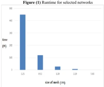
in order to determine the independence and dependence of the network solution in modeling the movement of the fluid column, in order to determine the sensitivity and optimal network access to solve, five computational networks are considered. In the direction of the coordinate, the direction of flow, the x axis and the direction of the depth of the flow, is the y axis. Table (1) shows the network size, number of nodes and number of elements for the five listed states.
Table (1) Selected computational grid view Name Mesh size
(centimeters) Number of nodes Number of elements
M-1 0.25 360267 356600
M-2 0.5 91035 89200
M-3 1 23218 222300
M-4 2 6258 5798
M-5 5 1074 890
62 As we can see, with the mesh being smaller, the implementation time of the model increases significantly. It should be noted that by halving the size of mesh in a network, the number of elements of the model is quadrupled, and approximately the same proportion is expected to increase the execution time of the program as well.
Figure (1) Runtime for selected networks
In order to compare the results of the fluid flow profile generated by the fluid column movement, various networking results with laboratory values have been used. For quantitative evaluation and comparison of experimental results with model results in different network sizes, the error values are calculated from the relation 1:
rror ∑ i i i
i
In this regard, " " is the number of data, " " _ "i" the quantity obtained from the present model and " " _ "i" ^ "'' is also the amount of quantity that is available from the experimental study. Table (2) shows the error rate for each of the selected networks.
Table 2 shows the error rate results for five networking modes
M-5 M-4 M-3 M-2 M-1 Name of the
network 21/46 13/07 8/78 6/63 6/01 Error rate
According to the above table, it is seen that M-5% has a high error, but the M-3 network and smaller, the percentage error does not change much. But only the percentage of error in choosing the best networking standard is not enough and it should also consider the computational cost of the model. According to the above, the M-3 networking is considered as the most appropriate and optimal option both in terms of both the implementation time and the error rate, and then the networking is used for modeling.
3. RESULTS AND DISCUSSION
As mentioned in the introduction, the effect of the barrier and the environmental conditions of the bed on the movement of the fluid column will be investigated in the present study. The environmental conditions of the substrate are defined as dry substrate and wet substrate. Also, to investigate the impact of the obstacle, the type of sharp edges was used. To simulate the movement of the fluid column from the dry and wet substrate, the results of the experiments were performed using Azeman and Cocamen [13]. The experiments are carried out in two different conditions: in the first test, the substrate is lower than the dry canal and in the second test, the substrate is wet and the depth is 025 m. The initial model conditions for a dry bed are shown in Fig.2.
Figure (2) The initial conditions of the model of movement of the fluid column in the dry bed
The results of the dry bed test indicate that the flow of the valves moves with a curve downstream after removing it. Over time, curvature decreases and the flow attempts to balance the potential difference before and after the valve. Numerical modeling results confirm this and are in good agreement with experimental results. Comparison of numerical and laboratory results is shown in Fig. 3. It should be noted that the coordinate axes with the parameter h, which is 0.25 in this case, and the time is also t t√ (g / h). The velocity in the forehead of the wave is also maximized and increases over time.
Fig. 3 Comparison of the measured water surface profile in the laboratory and calculated by the finite volume method for dry substrate a) T = 1.13
b) T = 2.76 c) T = 3.88 d) T = 5.01 e) T = 6.64 A)
c)
d)
e)
As mentioned, in the next modeling, the bottom of the canal is not at the bottom of the bottom and is at a height of 0.025 meters. The initial conditions of this model are shown in Fig. 4.
Figure (4) An overview of the initial conditions of the movement model of the fluid column in the
wet bed
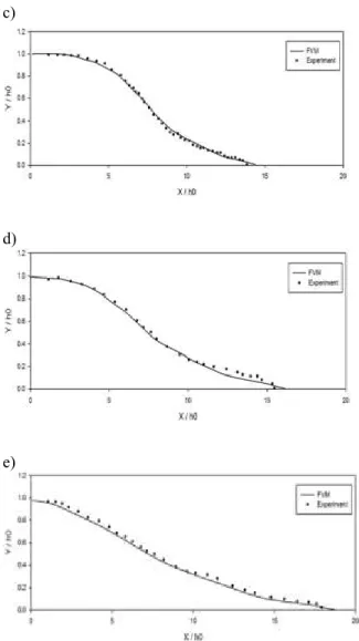
The results of the wet bed test show that, after removing the valve, the inflow flow from the reservoir encounters the downstream stream and the result of this collision creates a peak of flow in the collision, which in turn increases the depth of the flow. Over time, as the dry bed, the curvature of the flow in the upstream decreases, but the peak formed at the intersection crosses downwards and covers a wider range. Fig. 5. The results of numerical modeling show that the model shows the peak height of the peak at the intersection
and with the passage of time in the lower part of the experimental state, which has a significant adaptation due to its conformance.
Fig. 5: Comparison of water level profiles in laboratory and calculated by finite volume method for
wet substrate A)
b)
c)
d)
e)
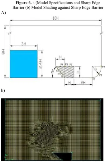
64 laboratory results in this field, numerical results have been used with finite difference method and compared with the results of the present study [14]. To simulate, a two-dimensional channel with a length of 1 meter and a height of 0.8 m is modeled with a dry bottom. From the wall of the channel to 0.3 m away, the water column is at a height of 0.24 m. The channel's end is also considered as far away as possible, so that the volume of the fluid can continue in the proper time without colliding with any other obstacle. Figure 6a shows the characteristics of the model and Figure 6b illustrates a view of the pattern of the constructed model. The parameter H for the modeling in Figure 6a is 0.1.
Figure 6. a (Model Specifications and Sharp Edge Barrier (b) Model Shading against Sharp Edge Barrier A)
b)
The results of modeling by the finite volume method are compared in Fig. 7 with the results of the finite difference method. As can be seen, after the collapse of the water column, a flood wave is created. Due to the collision of this flood wave to the obstacle, a complex flow pattern is formed. Flow failure occurs when flow is blocked. As a large part of it is reflected, it moves upwards in the form of a negative wave. On the other hand, this reversal wave causes an increase in the height of the stream in the upstream and, by increasing the specific energy, prevents the flow of the barrier. By comparing the two-way diagrams, it can be seen that the results of the two methods of finite difference and finite volume in the indicated times are in good agreement. It should be noted that, for longer times, the results of two numerical models are not very
consistent, which can be due to the extreme changes in the acceleration of the flow at very low times.
Fig. 7. Comparison of water surface profiles for sharp edges using a finite difference and finite volume
method. T = 1.63 b) T = 3.53 a)
b)
Figure 8a shows the flow pressure contour at the instant of the collision of the fluid and the shape (8) -b, and the parameter α represents the boundary between the two phases of the air. It is observed that the maximum pressure at the intersection of the obstacle flow occurs due to the extreme velocity of the velocity.
Figure 8 a)Constant flow pressure at the moment of collision flow to the obstacle (b) The value of the
4. CONSLUSION
In the present study, the movement of the fluid column under the influence of dry and wet substrate and with the presence of sharp edges was investigated. For this purpose, a finite volume numerical method was used and OpenFOAM software was used for modeling. Gambit software was used to build geometry and mesh the model. Before constructing different models, the numerical solution independent evaluation of the results was first examined. Finally, according to the accuracy and execution time of the programs, the network is selected with a mesh size of 0.01 meters. In the course of its erosion, a water box was modeled in dry and wet substrate conditions. In dry bed conditions, there is good agreement between the numerical and experimental models and the program has been able to model the sudden acceleration resulting from the pillar drop. In the case where the bed is not dry, the collision of two moving and moving fluid regions causes a flush to appear in the corresponding diagrams. These steps are well simulated by the code and the results are verified. In the obstruction model, because of the particular barrier shape, the flow pattern is very complex and part of the current is reflected in the form of a return wave and part of it is divided into the following parts in combination with air. The bounce wave causes an increase in the upstream flow of the stream and, by increasing the specific energy, prevents the flow of the barrier. In general, we can conclude that the two-phase model in the simulation of the motion of the fluid column is successful in two-dimensional and can be developed for similar phenomena of the present model.
FUNDING/SUPPORT
Not mentioned any Funding/Support by authors.
ACKNOWLEDGMENT Not mentioned.
AUTHORS CONTRIBUTION
This work was carried out in collaboration among all authors.
CONFLICT OF INTEREST
The author (s) declared no potential conflicts of interests with respect to the authorship and/or publication of this paper.
5.REFERENCES
1-Fraccarollo, L., & Toro, E. F. (1995). "Experimental and numerical assessment of the shallow water model for two-dimensional dam-break type problems". Journal of Hydraulic Research, Vol. 33(6),143-164. [scholar]
2-Ferrari, A., Fraccarollo, Dumbser, M., Toro, E., & Armanini, A. (2012). "Three dimensional fllow evolution after a dam break". J. Fluid Mech. 663, 456-477. [scholar]
3-Yang, C., Lin, B., Jiang, C., & Liu, Y. (2012). "Predicting near-field dam-break flow and impact force using a 3D model". Journal of Hydraulic Research, Vol. 41(6), pp 714-792. [scholar] 4-Biscarini, C., Francesco, D., & Manciola, P. (2012).
"CFD modelling approach for dam-break flow studies". Hydrol. Earth Syst. Sci. 14 (4), 725-711. [scholar]
5-Singh, J., Altinakar, M., & Ding, Y. (2011). "Two-dimensional numerical modeling of dam-break flows over natural terrain using a central explicit scheme". Advances in Water Resources, 1366– 1375. [scholar]
6-Bellos, V., & Hrissanthou, V. (2011). "Numerical Simulation of a Dam-Break Flood Wave". European Water 33 , 45-53. [scholar]
7-Marsooli, R., Zhang, M., & Wu, W. (2011). "Vertical and horizontal two-dimensional numerical modeling of dam-break flow over fixed beds". Proceedings of World Environmental and Water Resources Congress, ASCE, Palm Springs, CA., U.S.A. [scholar]
8-Oertel, M., & Bung, D. (2012). "Initial stage of two-dimensional dam-break waves:laboratory versus VOF". Journal of Hydraulic Research, Vol. 52(1), pp 19-97. [scholar]
9- VAGHEFI, M., SHAKERDARGAH, M., & AKBARI, M. (2015). Numerical investigation of the effect of Froude number on flow pattern around a submerged T-shaped spur dike in a 90 bend. Turkish Journal of Engineering and Environmental Sciences, 38(2), 266-277. [scholar]
10- Shih, T. H., Liou, W. W., Shabbir, A., Yang, Z., & Zhu, J. (1995). A new k-ϵ eddy viscosity model for high reynolds number turbulent flows. Computers & Fluids, 24(3), 227-238. [scholar] 11- Bremhorst, K. (1981). A modified form of the
ke model for predicting wall turbulence. Journal of fluids engineering, 103, 457. [scholar]
12- Ozmen-Cagatay, H., & Kocaman, S. (2010). "Dam-break flows during initial stage using SWE and RANS approaches". Journal of Hydraulic Research, Vol. 41(5), pp 623-611. [scholar] 13- Marrone, S. (2012). Enhanced SPH modeling of
66 14- Sadeghi, M., Thomassie, R., & Sasangohar, F.
(2017, June). Objective Assessment of Patient Portal Requirements. In Proceedings of the International Symposium on Human Factors and Ergonomics in Health Care (Vol. 6, No. 1, pp. 1-1). Sage India: New Delhi, India: SAGE Publications. [scholar]
15- Khanade, K., Sasangohar, F., Sadeghi, M., Sutherland, S., & Alexander, K. (2017, September). Deriving Information Requirements for a Smart Nursing System for Intensive Care Units. In Proceedings of the Human Factors and Ergonomics Society Annual Meeting (Vol. 61, No. 1, pp. 653-654). Sage CA: Los Angeles, CA: SAGE Publications. [scholar]
16- Sadeghi, M., Thomassie, R., & Sasangohar, F. (2017, September). Objective Assessment of Functional Information Requirements for Patient Portals. In Proceedings of the Human Factors and Ergonomics Society Annual Meeting (Vol. 61, No. 1, pp. 1788-1792). Sage CA: Los Angeles, CA: SAGE Publications.[scholar]
17- Sadeghi, M., & Sasangohar, F. (2018, September). Investigating Nursing Task Interruptions in Intensive Care Units: A Scoping Literature Review. In Proceedings of the Human Factors and Ergonomics Society Annual Meeting (Vol. 62, No. 1, pp. 478-479). Sage CA: Los Angeles, CA: SAGE Publications. [scholar] 18- Sadeghi, M., Khanade, K., Sasangohar, F., &