A SIMPLIFIED PROCEDURE OF LINEAR REGRESSION IN A PRELIMINARY ANALYSIS
S. Facchinetti, U. Magagnoli
1. INTRODUCTION
The use of the inferential statistical methodologies needs frequently to define preliminary procedures in order to choose a probabilistic model that has to be used in a second stage of the study. The aim of this study is to solve inferential problems of estimation, especially in case of large data set of observations, such as in economic, physical, biological, enviromental and technological fields.
In fact, from a point of view economic and methodologic, it seems useful to choose in a preliminary stage the models and examine them closely, with more complex methods, in a second stage. For example, in financial field large data sets referred to the different characteristics of the stocks, whose structural links have to be studied, are present. Furthermore, also in biology, large data sets have to be examined, in particular in the observation or in the experimental analyses.
This preliminary stage, that usually is called “identification of the model”, con-sists in two components: structural and stochastic; it is better using simplier methodologies than the one of the likelihood, either from a formal point of view or a computational one. Indeed, in this way many optimal asymptotical properties of the likelihood procedure are lost. Consequently, the use of simplified methods must be evaluated in terms of efficiency loss, comparing, when possible, the in-formation matrix or, simply, the variance or mean square error of the estimated parameters, always considering the unbias and verifying the consistency.
These simplified methods can be applied in order to define the dependence, not fixed in a parametric form, of a curve or a surface; or even when it is neces-sary substituting complex computations with simplier ones (Cox, 2006).
Moreover, our purpose is to evaluate the median applications of the different subsets of observed values, instead of the location index usually represented by the mean. This kind of procedure is useful in case of anomalous values, given by particular types of observation contaminations. Therefore, this method can be considered as a simplified one in the subject of the “robust” regression (Huber and Ronchetti, 2009).
verify the properties of the estimator regression coefficients, obtained by the simplified procedure. To obtain the regression function we use either the ordered means or the ordered medians. In particular, a polynomial structure of the first and the second order has been considered, in order to define the functional link between the two variables. Furthermore, it has been assumed that the random variable X and the error component, defined in the regression model, have a normal distribution.
In the third paragraph the results of the estimations obtained varying the pa-rameters of the procedure for the polynomial model either of the first and the second order are presented. A reduced number of data than in the real analysis has been considered in details, because it allows to underline the limits of the procedure and some anomalous situations that can happen. Therefore a compari-son between the simulation results and the one obtained by the ordinary least squares procedure is carried out.
Finally, the fourth paragraph gives some remarks about the statistical proper-ties of the proposed procedure, in particular, with relation to the consistency of the estimators of the regression coefficients for the first and the second order models.
2. MODEL, ASSUMPTIONS AND SIMPLIFIED PROCEDURE
Let (X, Y) be the two characteristics of interest whose n observations: Sn = {(xi, yi); i = 1, 2, ..., n} are known. In most cases the two random variables X and Y may be chosen in a set (X1, X2, ..., Xg) of large size g. In particular X is the re-gressor or explicative variable and Y is the regressed one, whose behaviour will be studied related to X by the model:
( )
Y y X (1)
where is the error component, independent of X, with E() = 0, Var() = 2.
The regression function y(x), that generally belongs to the complete polyno-mial family of order r, is estimated by:
0
( ) r s
r sr
s
y x a x
(2)with asr 1 and arr 0 gathered in the vector ar = (a0r,..., arr)’ of the parameters
of order (r +1) 1.
The y(x) function and the variance of the error component 2 can be see
re-spectively as conditioned mean E{Y|x} and conditioned variance Var{Y|x} (that is assumed as constant).
X = 0 and X2 = 1, without loss of generality, and N(ε, 2), with parameters ε = 0 and ε2 costant.
The proposed regression simplified procedure consists of four steps.
1. Let have n observations of the bivariate random variable (X, Y), Sn = {(xi, yi); i = 1, 2, ..., n}, ordered for the increasing values of X (xixi+1), in
the interval In = [mini (xi); maxi (xi)] [x1; xn].
2. The data set Sn is partitioned in m 2 subsets S[j] for j = 1, 2, ..., m, of size
[ ]j /
n n m or n[ ]j n m/ 1 nearly constant, with [ ] 1
m j j
n n
,defin-ing u the whole part of u, with [ ]
1
m
j n
j
S S
and Sj Sk = for j k. Each subset is formed by the couples (xi, yi) Î Sn according to the relation:[ ]j {( , ) :i i [j 1] [ ]j }
S x y N i N
where [ ] [ ]
1
j
j k
k
N n
and N[0] = 0.3. For each subset S[j] the observations are synthesized by the “mean” or by the “median”:
[ ]j Mean( :i i [ ]j ), [ ]j Mean( :i i [ ]j )
x x x S y y y S
[ ]j Median( :i i [ ]j ), [ ]j Median( :i i [ ]j )
x x x S y y y S (3)
obtaining the points P[ ]j (x[ ]j , y[ ]j ), specifically signed P[ ]j (x[ ]j , y[ ]j ) or P[ ]j (x[ ]j ,y[ ]j ).
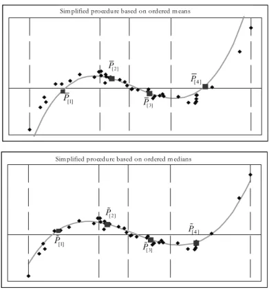
4. The so located points P[ ]j (or P[ ]j ) in 2 give a “piecewise-linear
regres-sion” of (m – 1) consecutive segments which can be assumed as a prelimi-nary estimation of the regression function y(x). Assuming a polynomial of order r = m – 1, it is possible a fitting through the m points P[ ]j or P[ ]j that define “the regression procedure ordered by means or by medians”, respectively. The parameters (regression coefficients) are obtained as the solutions of the following system of m linear equations in r + 1 unknown quantities:
[ ] [ ]
0
( ) r s for 1, 2,...,
j sr j
s
y x a x j m
or as a matrix:
[.] [.] r
y P a (5)
where y[.](y[1], y[ 2],..., y[ ]m )' is the m 1 vector of y[ ]j , with y[ ]j equal to y[ ]j or y[ ]j , ar (a0r,...,arr)' is the (r + 1) 1 vector of the regression coefficients and P[.] is the m (r + 1) invertible square matrix of x[ ]j (x[ ]j or x[ ]j ) powers:
[ ]
{pjs xsj ;j 1, 2,..., ; m s 0,1,..., }r
[.]
P .
As the P[.] matrix is invertible by construction, the vector of the
coeffi-cient estimators ar is
1
r [.] [.]
a P y (6)
that gives the estimations of ar or ar, if we consider P[ ]j or P[ ]j , for j = 1, 2, ..., m.
If we may suppose that the polynomial function y(x) has given by means of a polynomial in x of order r
0
( ) r s with (1 r)
r sr
s
y x a x ,x,...,x '
' r
a x x (7)
the proposed procedure allows to obtain the regression coefficient estimation ar,
referred to the use of the P[ ]j points for j = 1, 2, ..., m “means” (P[ ]j ) or “medi-ans” (P[ ]j ), respectively.
In this preliminary explorative research we study the polynomial functions of order r = 1 and r = 2 for their general approximation to the y(x) function (Taylor theorem).
The polynomial function defined in (2) can be expressed by a series of or-thogonal polynomial. In particular, among the different groups of oror-thogonal polynomials, we have considered the Hermite ones, relating to the possible values assumed by X (-, +) and under the assumption of normal distribution for the values of the random variable X, whose standardized density function is consis-tent with the weight function w(x) = exp (-x2).
Figure 1 – The proposed simplified procedure: an example for n = 30, m = 4, r = 3.
2 2
( ) ( 1)r x r x
r r
d
h x e e
dx
. (8)
In particular, for r from 0 to 5:
0
1
2 2
3 3
2 4
4
3 5
5
( ) 1 ( ) 2
( ) 2 4
( ) 12 8
( ) 12 48 16
( ) 120 160 32
h x
h x x
h x x
h x x x
h x x x
h x x x x
and the polynomial function is
0
( ) r ( )
r s s
s
y x c h x
. (9)Proce du ra ordi n ata basata su lle m e die
[1]
P
[ 2]
P
[ 3]
P
[4 ]
P
Sim plified procedure based on ordered m eans
Proce du ra ordi n ata basata su ll e m e dian e
[1]
P
[ 2]
P
[ 3]
P
[4 ]
P
By the (8) and (9) equations some linear functions, synthesized in the Tr matrix
of order (r + 1) (r + 1), ar and cr ( , ..., )'c c0 1 cr coefficients are obtained the ones from the others. In particular, the coefficients ar of the polynomial of order
r in x are obtained by assigning values to cr, that defines the function y(x) in
terms of Hermite polynomials:
r r
a T cr . (10)
As Tr is a triangular matrix (r + 1) (r + 1) it is ever invertible, therefore it is
possible to obtain the estimations of the cr parameters, if the ar parameters, have been estimated by the proposed procedure:
1
r r
c T ar . (11)
In particular, for r from 0 to 5:
5
1 0 2 0 12 0
0 2 0 12 0 120
0 0 4 0 48 0
0 0 0 8 0 160
0 0 0 0 16 0
0 0 0 0 0 32
- - -
T
where the T0, T1,..., T4 matrixes are the sub matrixes of T5. For example T3 = {tks = tks T5, for k, s = 1, ..., 4}.
2.1. The first-order linear model
For r = 1 the regression function is y1(x) = a01 + a11x and the corresponding
random variable is Y = a01 + a11X + .
Under the assumption of normal distribution of X and , the random variable Y is normally distributed, too: Y N(Y, Y2), with Y = a01 + a11X and Y2 = a112X2 + 2.
The bidimensional random variable (X, Y), whose observations {(xi, yi), i = 1, 2, ..., n} give a random simple sample of size n, is binormally distributed N2[(X,
Y), (X2, Y2, XY = XY)] with covariance XY = a11X2. Therefore, the pa-rameters of the regression function y1(x) are given as function of those of the
bi-normal random variable (X, Y):
01 Y 11 X Y Y X
X
a a
11 Y
X
a
In this case the data set Sn, ordered for increasing value of X, is partitioned in two subsets (m = 2) of equal size (nearly n/2). Then a straight line is drawn through the two points P[j] , j = 1, 2: considered the ordered “mean” values P[ ]j or the “median” ones P[ ]j .
To verify the statistical properties of the estimators aˆ01 and aˆ11, for (X, Y) a standardised binormal distribution with X = Y = 0 and X2 = Y2 = 1 is as-sumed, having XY = , a01 = 0 and a11 = .
Moreover, replacing the Y with the X and ordering the data set Sn for increas-ing values of Y, the estimations of the regression coefficients of the straight line x1(y) = b01 + b11y can be obtained.
The estimation of results
11 11 11
11 11 11 11 11
11 11
ˆ
ˆ
ˆ ˆ
1 (or 1) if sign( )( ) 1 (or 1)
ˆ ˆ
ˆ ˆ ˆ
sign( ) if 0 1
ˆ ˆ
0 if sign( ) sign( ) 0
a a b
a a b a b
a b
where sign( )a a a/ for a0.
2.2. The second-order linear model
For r = 2 the regression function is y2(x) = a02 + a12x + a22x2 and the
corre-sponding random variable is Y = a02 + a12X + a22X2 + . Under the given
distri-bution assumption for the random variable X and the error component , with-out loss of generality, we can assume X = 0 and X2 = 2 = 1; applying the
sim-plified procedure for ordered “means” or “medians”, the data set Sn is partitioned into three subsets (m = 3) of equal size (nearly n/3) and the three points result
[ ]j
P for j = 1, 2, 3.
2.3. Statistical properties of the regression coefficients obtained by the simplified procedure In this section, some considerations on the consistency of the estimators of the regression coefficients, obtained by the proposed procedure, are given.
We know that to verify the consistency, the variances of the estimators need to tend to zero, when n diverges, and under the stated distributive assumption, it oc-curs. Therefore, we only verify the asymptotic unbias of the estimators.
In particular, when r = 1 and n diverges, the two ordered data subsets S[1] and
[ 2]
S show higher or lower values, respectively, than the threshold value, that for the random variable X corresponds to the 50th percentile. Moreover, since X
abscissas of the points P[1] and P[ 2] (x[1] and x[ 2]) are, when n diverges, means
of a truncated random variable:
[1] | 0 ; [ 2] | 0
x E X X x E X X .
For the properties of the normal distribution of a standardised truncated ran-dom variable we have
(0) 2 2 2
{ | 0} { | 0}
(0) 2
E X X E X X
(13)
where (z) and Φ(z) are the probability distribution function and the cumulative distribution function of the standardised normal random variable, respectively.
The ordinates of the points P[1] and P[ 2] ( y[1] and y[ 2]) are, when n diverges, the conditioned means of the random variable Y:
[1] 01 11
01 11 01 11 [1]
{ | 0} { ( | 0) }
( | 0)
y E Y X E a a X X
a a E X X a a x
with E{} = 0, and
[ 2] { | 0} 01 11 [ 2]
y E Y X a a x .
The simplified procedure allows to obtain the convergence values of the esti-mators aˆ01 and aˆ11 as the solutions of the system of the equations:
[1] 01 11 [1]
[ 2] 01 11 [ 2]
ˆ ˆ
ˆ ˆ .
y a a x
y a a x
They coincide with the parameters a01 and a11 of the model, so the estimates
are consistent.
When r = 2 and n diverges, the three ordered data subsets S[1], S[ 2] and S[ 3]
are characterised by two values of threshold corresponding to the 33.3th
percen-tile and to the 66.7th percentile. By the given assumption of X as standardised
normal random variable, the threshold values are, respectively:
x33.3% = Φ(0.333) = -0.43073 = -zs and x66.7% = Φ(0.667) = 0.43073 = zs.
The abscissas x[1], x[ 2] and x[ 3] of the three points P[1], P[ 2] and P[ 3], when n
[1] { | s}; [ 2] { | s}; [ 3] { | s}
x E X X z x E X X z x E X X z . (14)
Furthermore, for the properties of the standardised truncated normal distribu-tions (Johnson, Kotz and Balakrishnan, 1994-1995), we have
( )
{ | } -1.0908
1/3
{ | } 0
{ | } 1.0908.
s s
s
s
z
E X X z
E X X z
E X X z
Hence:
[1] 1.0908 [ 2] 0 [ 3] 1.0908
x x x . (15)
The second order moments of the three truncated normal random variables are
2
2 2
2 2
3 3 3
{ | } { | } , 1.4698
2 2 2
2 3
{ | } , 0.0603
2 2 /3 s s s s s z
E X X z E X X z
z
E X X z
(16)
where Γ(a) and Γ(a, u) are the Gamma and incomplete Gamma functions, respec-tively.
The y[1], y[ 2] and y[ 3] ordinates of the three points P[1], P[ 2] and P[ 3], when
n diverges, correspond to the expected values of Y = a02 + a12X + a22X2, where
the conditioned means of X and X2, before defined, have placed instead of X and
X2:
2
[1] 02 12 22
2
[ 2] 02 12 22
2
[ 3] 02 12 22
{ | } { | } { | }
{ | } { | } { | }
{ | } { | } { | }.
s s s
s s s
s s s
y E Y X z a a E X X z a E X X z
y E Y X z a a E X X z a E X X z
y E Y X z a a E X X z a E X X z
(17)
The aˆ02, aˆ12 and aˆ22 regression estimator coefficients are obtained by the
“ordered means” procedure as solutions of the following linear system:
2
[1] 02 12 [1] 22 [1]
2
[ 2] 02 12 [ 2 ] 22 [ 2]
2
[ 3] 02 12 [ 3] 22 [ 3]
ˆ ˆ ˆ
ˆ ˆ ˆ
ˆ ˆ ˆ .
y a a x a x
y a a x a x
y a a x a x
Subtracting the respective equations of the (17) from the (18) and remember-ing the results of the (15):
2 2
02 02 12 12 [1] 22 [1] 22
2
02 02 22
2 2
02 02 12 12 [1] 22 [1] 22
ˆ ˆ ˆ
( ) ( ) { | } 0
ˆ
( ) { | } 0
ˆ ˆ ˆ
( ) ( ) { | } 0.
s
s
s
a a a a x a x a E X X z
a a a E X X z
a a a a x a x a E X X z
Furthermore, when n diverges, from (16) it is possible to obtain the estimators
02
ˆ
a , aˆ12 and aˆ22, as function of a02, a12 and a22:
2
02 02 22 02 22
12 12
2 2 2
22 22 [1] 22
ˆ { | } 0.0603
ˆ
ˆ [ { | } { | }/ ] 1.1846 .
s
s s
a a a E X X z a a
a a
a a E X X z E X X z x a
(19)
We note that the estimators aˆ02 and aˆ22 do not result consistent, while aˆ12 converges to the corresponding parameter, when n diverges.
So we have to evaluate the bias of the estimators.
In particular, if the Hermite coefficients are c0 = c1 = 0 and c2 = 1,
correspond-ing to the parameters a02 2, a12 0, a224 and the mean values of the
es-timators aˆ02, aˆ12 and aˆ22 are equal to:
02
ˆ
a = -1.7587
12
ˆ a = 0
22
ˆ
a = 4.7385.
3. NUMERICAL SIMULATION: SOME RESULTS
In order to give not only methodological indications, but also operative ones, a Monte Carlo numerical simulation has been carried out.
The aim is to obtain the distribution of the estimator parameters of the poly-nomial model, to evaluate their properties and to compare them with the corre-sponding parameters obtained by the least square method.
To underline the properties of the simplified procedure N = 1000 replications have been made. Moreover, to emphasise the bias and the dispersion of the esti-mated parameters, we have considered low sample size n = 10, 20, 30.
The models and the basic assumptions are those specified in the second para-graph, with particular reference to the polynomial models of order r = 1 and r = 2.
3.1. The first-order linear model
For the polynomial of the first order, we have considered equal to 0, 0.25, 0.5 and 0.751. The simplified procedure is the one given in paragraph 2.1..
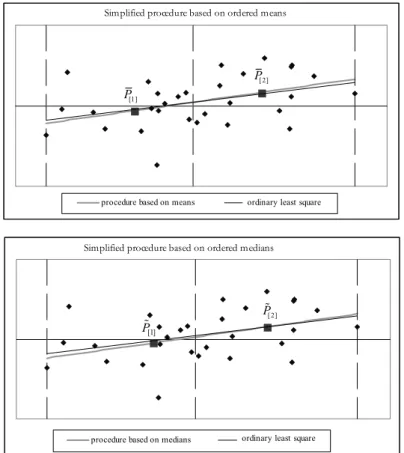
In particular, for n = 30 and = 0.5 the following Figure 2 shows the esti-mated models, considering the results obtained by the “means” procedure and by the “medians” procedure, with a comparison with the results obtained by the or-dinary least square method.
Figure 2 – The proposed simplified procedure: an example for n = 30, m = 2, r = 1.
In the graphs we can observe the partition in two subsets (m = 2) of size n/2 and the mean and the median points of each subset that define the models.
1 The results obtained by simulations for > 0 are equivalent to the corresponding ones for
< 0 and therefore it is not necessary to analyse them.
Procedura ordinata basata sulle medie
procedure based on means ordinary least square Lineare (dispersione)
[1]
P
[ 2]
P
Procedura ordinata basata sulle mediane
procedure based on medians Lineare (dispersione)
[1]
P
[ 2]
P
ordinary least square
Simplified procedure based on ordered means
To verify the fitness of the proposed procedure, the tables 1, 2 and 3 give, for some values of n and , the bias and the standard deviations (SD) of the esti-mated parameters for the ordered means procedure, the ordered medians proce-dure and the least square method, respectively.
The tables give only the values of the estimates of the regression coefficients for the function y1(x) = a01 + a11x, because those referred to the function x1(y) =
b01 + b11y are quite similar.
TABLE 1
Synthesized results of the simulation referred to the simplified procedure based on ordered means: N = 1000, r = 1
01
ˆ
a aˆ11 ˆ
n BIAS SD BIAS SD BIAS SD
0 0.009 0.352 0.000 0.483 0.003 0.353
0.25 0.008 0.341 0.000 0.467 -0.030 0.344
0.5 0.009 0.294 0.000 0.328 -0.019 0.257
10 10 10
10 0.75 0.006 0.233 0.000 0.319 -0.031 0.232
0 0.005 0.236 0.006 0.299 0.004 0.241
0.25 0.005 0.228 0.006 0.289 -0.021 0.236
0.5 0.004 0.204 0.006 0.259 -0.022 0.221
20 20 20
20 0.75 0.003 0.156 0.004 0.197 -0.013 0.149 0 0.004 0.188 0.009 0.237 0.008 0.192
0.25 0.004 0.182 0.009 0.229 -0.013 0.199
0.5 0.004 0.163 0.008 0.205 -0.008 0.172
30 30 30
30 0.75 0.003 0.124 0.006 0.157 -0.006 0.115
TABLE 2
Synthesized results of the simulation referred to the simplified procedure based on ordered medians: N =1000, r = 1
01
ˆ
a aˆ11 ˆ
n BIAS SD BIAS SD BIAS SD
0 0.018 0.452 0.019 0.745 -0.006 0.485
0.25 0.018 0.446 0.064 0.737 -0.009 0.470
0.5 0.012 0.421 0.105 0.683 0.006 0.416 10
10 10
10 0.75 0.010 0.345 0.119 0.556 0.020 0.296
0 0.011 0.280 0.011 0.424 0.007 0.355
0.25 0.011 0.274 0.055 0.413 0.021 0.327
0.5 0.010 0.255 0.087 0.385 0.037 0.284 20
20 20
20 0.75 0.005 0.215 0.103 0.327 0.054 0.183
0 0.004 0.237 0.015 0.354 0.010 0.300
0.25 0.001 0.236 0.065 0.347 0.032 0.286
0.5 -0.002 0.221 0.100 0.327 0.058 0.242 30
30 30
30 0.75 0.002 0.185 0.120 0.286 0.074 0.150
TABLE 3
Synthesized results of the simulation referred to the ordinary least square method: N = 1000, r = 1
01
ˆ
a aˆ11 ˆ
n BIAS SD BIAS SD BIAS SD
0 0.010 0.340 0.000 0.378 -0.002 0.329
0.25 0.010 0.329 0.000 0.366 -0.013 0.310
0.5 0.009 0.294 0.000 0.328 -0.019 0.257 10
10 10
10 0.75 0.007 0.225 0.000 0.250 -0.018 0.169
0 0.006 0.232 0.000 0.232 -0.002 0.219
0.25 0.005 0.225 0.000 0.224 -0.005 0.205
0.5 0.005 0.201 0.000 0.201 -0.008 0.169 20
20 20
20 0.75 0.004 0.153 0.000 0.153 -0.008 0.106
0 0.005 0.186 -0.010 0.180 0.000 0.177 0.25 0.005 0.180 -0.001 0.175 -0.161 0.087
0.5 0.004 0.161 -0.001 0.156 -0.006 0.135 30
30 30
We can observe that the estimator parameters defined by the means procedure present a smaller bias than those based on the medians. Moreover in the three tables there are two particular situations in which the value assigned to the es-timates has conventionally defined:
1. when the product of the estimated regression coefficients exceed the unity: in this case ˆ is assumed equal to 1 according to the common sign of the two coefficients;
2. when the product of the estimated regression coefficients is negative: in this case ˆ is assumed equal to 0.
The distribution of the estimators, obtained by simulation, has characteristics referring to a mixture variable with two components: one continuous and one discontinuous. Furthermore, it allows to evaluate the fraction of simulations number in which the situations 1. and 2., corresponding to the discontinuous variable, happen.
In Table 4 the quantities in the N = 1000 simulations with ˆ equal to – 1, 0, 1, referred to the two simplified procedures by ordered means and medians, are given.
TABLE 4
Simulations number with ˆ= -1, 0, 1 for N = 1000
Procedures by ordered means Procedures by ordered medians
n ˆ = -1 ˆ = 0 ˆ = 1 ˆ = -1 ˆ = 0 ˆ = 1
0 4 289 13 4 0 16
0.25 0 251 20 0 0 30
0.5 0 119 41 0 0 80
10 10 10
10 0.75 0 19 150 0 0 266
0 0 289 0 0 178 0
0.25 0 184 1 0 120 1
0.5 0 51 3 0 43 7
20 20 20
20 0.75 0 0 15 0 5 76
0 0 267 0 0 0 0
0.25 0 144 0 0 0 0
0.5 0 13 0 0 0 2
30 30 30
30 0.75 0 0 0 0 0 38
We observe that, considering models with theoretical values > 0, for ˆ = -1, the number of simulations is nearly zero for both the proposed procedures, since only for n = 10 and = 0 there is a number of simulations equal to 4 on 1000. Instead, for ˆ = 1 we observe that the number of simulations notably decreases at the increasing of n and at the decreasing of the correlation coefficient . In par-ticular, for = 0.75 and n = 10 the number of simulations is 150, for the ordered means procedure, and 260 for the ordered medians procedure. For n = 30 the number of simulations is reduced to 0 and 38, respectively.
is odd (n/2 = 5 and 15, respectively), hence the medians of the subgroup (in terms either of x and y) are directly located by a point in the plane (x, y). On the contrary, for a number of subsamples as n = 20, the median point is located by the half-sum of the two central values, observed for the x and for the y, in the subsamples themselves. Such different behaviour can be observed in Table 5, in which the number of simulations is considered for ˆ = 0, n/2 = 5, 6, ..., 15 and = 0 and 0.75, that confirms the results in Table 4.
TABLE 5
Simulations number with ˆ= 0 for N = 1000 and n/2 = 5, 6, ..., 15
n/2 =2 k+1 ˆ = 0 n/2=2k ˆ = 0
0 0 0 218
5
5 0.75 0 6 6 0.75 26
0 0 0 185
7
7 0.75 0 8 8 0.75 4
0 0 0 178
9
9 0.75 0 10 10 0.75 5
0 0 0 157
11
11 0.75 0 12 12 0.75 2
0 0 0 147
13
13 0.75 0 14 14 0.75 0
0 0
15
15 0.75 0
Moreover, referring to the most important parameter a11, the relative
efficien-cies 2 / 2
OLS
are calculated, where 2 is the variance of the estimator 11
ˆ a , ob-tained by the proposed procedure, and 2
OLS
is the variance of the same estimator obtained by the ordinary least square method.
The results are given in Table 6.
TABLE 6
Relative efficiencies of a obtained by the proposed procedure (means or medians) in comparison ˆ11
with the ordinary least square method
n Relative efficiency obtained by the mean procedure Relative efficiency obtained by the median procedure
0 0.612 0.257
0.25 0.614 0.247
0.5 0.616 0.231
10 10 10
10 0.75 0.614 0.202
0 0.602 0.299
0.25 0.601 0.294
0.5 0.602 0.273
20 20 20
20 0.75 0.603 0.219
0 0.577 0.259
0.25 0.584 0.254
0.5 0.579 0.228
30 30 30
30 0.75 0.575 0.173
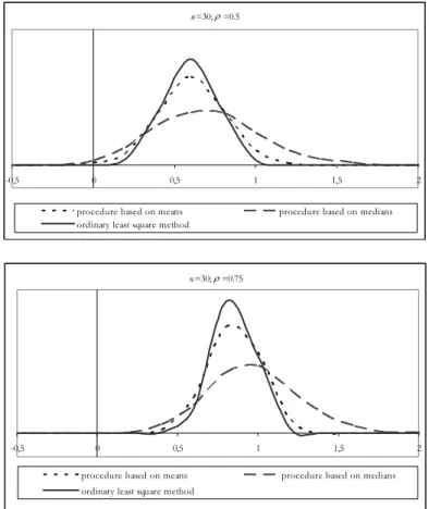
The next figure, that gives the distributions of the estimations of the parameter a11 obtained by the three methods when n = 30 and = 0.5 and 0.75, confirms
those data.
Figure 3 – Empirical distribution of aˆ11 for N = 1000, n = 20 and = 0.5 and 0.75.
3.2. The second-order linear model
We consider only some situations because we have observed asymptotic dis-torsions, as shown in paragraph 2.3.. In particular, the results of the simulation for N = 1000 and n = 30, assuming as model the Hermite polinomial of the sec-ond order with c0 = c1 = 0 and c2 = 1, corresponding to a02 2, a120,
22 4
a are given.
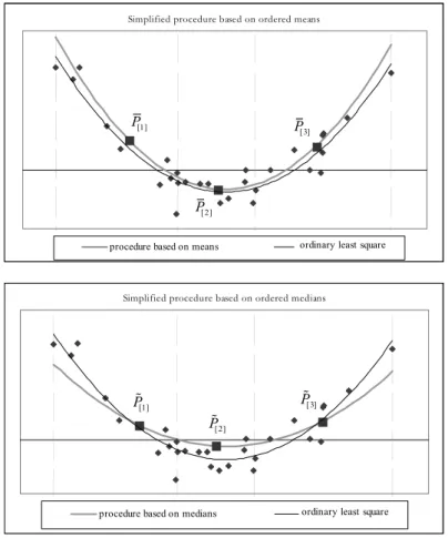
The Figure 4 shows an example of a model estimated by the proposed proce-dure, considering the ordered means and the ordered medians in comparison with the values obtained by the least square method.
n=30; =0.75
-0,5 0 0,5 1 1,5 2 procedure based on means procedure based on medians ordinary least square method
n=30; =0.5
-0,5 0 0,5 1 1,5 2
Figure 4 – The proposed simplified procedure: an example for n = 30, m = 3 and r = 2.
Specifically, we note the data partitioned in three subsets (m = 3) of size n/3, the mean and the median points of each subset that define the model.
Moreover, Table 7 gives some statistics referred to the estimations of the model parameters obtained by the ordered means procedure and the ordinary least square method.
TABLE 7
Synthesised results of the simulations referred to the simplified procedure based on the ordered means and to the ordinary least square method for N = 1000 and r = 2
Simplified procedure based
on ordered means Ordinary least square method
02
ˆ
a aˆ12 aˆ22 aˆ02 aˆ12 aˆ22
Mean -1.6939 0.0085 4.6625 Mean -1.9957 0.0011 3.9889
Median -1.7009 0.0063 4.6535 Median -1.9958 0.0046 3.9907
Variance 0.1357 0.2994 0.3604 Variance 0.0567 0.0452 0.0294
SD 0.3684 0.5472 0.6003 SD 0.2382 0.2126 0.1714
BIAS 0.3061 0.0085 0.6625 BIAS 0.0043 0.0011 -0.0111
MSE 0.2294 0.2995 0.7993 MSE 0.0568 0.0452 0.0295
Simplified procedure based on ordered means
procedure based on means Poli. (dispersione)
[1]
P
[ 3]
P
[ 2]
P
ordinary least square
Simplified procedure based on ordered medians
procedure based on medians Poli. (dispersione)
[3]
P
[2]
P
[1]
P
We observe that the bias of the estimates of the regression coefficients ob-tained by the proposed procedure are confirmed. In this case the estimates of a02
and a22 have values particularly high: 0.3061 and 0.6625 with respect to those
obtained by the least square method: 0.0043 and – 0.0111. The last values are only due to the casualness of the simulation procedure and to the dimension of the replications N = 1000. In fact, if we compare the mean values of the regres-sion coefficients obtained by simulation with those obtained in asymptotic condi-tions (see paragraph 2.3.), we have 0.0648 for a02 and – 0.0760 for a22. These
val-ues are really reduced, and therefore due only to the casualness of the simulation.
4. FINAL REMARKS AND CONCLUSIONS
The proposed simplified regression procedure can be useful in a preliminary stage to choose the polynomial regression model, because the partition of the data (x, y), referred to the explicative variable X, is defined relating to the number of the parameters of the chosen model. Hence in the general case the complete polynomial model is formed by m = r + 1 subsets, of size n/m. Therefore it is possible to start from the same data set to obtain the estimates of the regression models of order 1, 2, ..., r and to stop the procedure when the estimate of the re-gression coefficient arr has to be considered small ( ˆarr 0).
To state the order r of the regression polynomial, the “step-wise” procedure can be made like in the ordinaty least square method. In particular it is possible to apply the Student’s t test or of the Snedecor’s F test to verify the null hypothesis arr = 0. Note that to use this procedure, the variance of the estimeted parameter arr has to be obtained by numerical simulations.
The preliminary study to evaluate the inferential properties of the proposed procedure, by ordered means or medians and restricted to the polynomials of or-der 1 and 2 , has already shown some characteristics of the estimators, but it seems necessary to verify the extension for polynomial models of higher order.
For the model of order r = 1, we do not observe a bias of the estimators and comparatively, there is a higher relative efficiency of the procedure based on the means in respect of that based on the medians. So, in this first study we have verified for the polynomial model of order r = 2 only the ordered means proce-dure. In such a situation, we have numerically found that the coefficient estima-tors are generally biased and we have given a theoretical demonstration.
Some observations, relating to the possibility to estimate the correlation be-tween the explicative variables X and Y, not only in the linear function y = a01 +
a11x but also in the analogous model x = b01 + b11y, by means of the simplified
procedure, are given in the paper.
Finally, we think that this study could be complete with:
the analysis of polynomial models of order higher than two;
research has considered normally distributed, independent of the explicative variable and homoscedastic;
the extension of the comparison to the use of a loss function of order 1 and comparing the inferential properties of the model parameter with the one ob-tained by the quantile regression;
the extension of the proposed methodology to the situation with more than one explicative variable.
Dipartimento di Scienze statistiche SILVIA FACCHINETTI Università Cattolica del S. Cuore – Milano UMBERTO MAGAGNOLI
REFERENCES
M. ABRAMOVITZ, I.E. STEGUM,(1972), Handbook of Mathematical Functions, 10th printing,
Na-tional Bureau of Standards, – United States Department of Commerce, Washington D.C., USA.
D.R. COX, (2006), Principles of Statistical Inference, Cambridge University Press, Cambridge,
UK.
P.J. HUBER, E.M. RONCHETTI, (2009), Robust Statistics, 2nd Edition, Wiley, New York, USA. N.L. JOHNSON, S. KOTZ, N. BALAKRISHNAN, (1994), Continuous Univariate Distributions, Vol. 1,
Wiley, New York, USA.
N.L. JOHNSON, S. KOTZ, N. BALAKRISHNAN, (1995), Continuous Univariate Distributions, Vol. 2,
Wiley, New York, USA.
SUMMARY
A simplified procedure of linear regression in a preliminary analysis