ANALYSIS OF MONOTONE AND NON-MONOTONE TRAVELING WAVES IN A SYSTEM FOR SOCIAL OUTBURSTS
Caroline Yang
A dissertation submitted to the faculty at the University of North Carolina at Chapel Hill in partial fulfillment of the requirements for the degree of Doctor of Philosophy in the Department of
Mathematics in the College of Arts and Sciences.
Chapel Hill 2018
c 2018 Caroline Yang
ABSTRACT
Caroline Yang: Analysis of Monotone and Non-monotone Traveling Waves in a System for Social Outbursts
(Under the direction of Nancy Rodríguez)
Rioting events in the last several years in the United States, such as the Ferguson riots of 2014 and the Baltimore riots of 2015, captured the attention of the entire nation and have increased scrutiny of racial and social tension. The strength and duration of these riots leads to a question: is there a mathematical model that can reproduce the spread and intensity of rioting behavior observed over time and space in events like these? The goal of this work is to prove the existence and stability of traveling wave solutions to a model for the spread of rioting and social outbursts given by a reaction-diffusion system which captures the relationship between two variables: intensity of rioting behavior and social tension. This model was first introduced by Berestycki, Nadal, and Rodríguez in 2015.
To prove the existence and stability of the traveling wave solutions, we use existence and stability theory for monotone systems. In the case of parameter values that yield a non-monotone system, we establish the stability of traveling wave solutions by proving that the spectrum of the linear operator is not located in the closed, deleted, right half plane. We analyze the spectrum of the linear operator by finding the essential spectrum, placing a bound on the location of the point spectrum, and numerically searching for point spectra within this bounded region using the Evans function.
To my parents, Raymond and Ann Yang, and to my fiancé, Michael Zimmerman. If I put into words the love and respect I have for you three,
ACKNOWLEDGEMENTS
I would first like to thank my advisor, Nancy Rodríguez, for her guidance, insight, patience, and support over the past three years. Her passion for mathematics is clear, and she is an amazing model of work-life balance...I seriously do not know how she does it all. I am very grateful for her taking me on as a student and supporting my work through NSF Award 1516778. This work would not have been possible without her and my other committee members: Henri Berestycki, Chris Jones, Jeremy Marzuola, and Katie Newhall. Thank you all for your encouragement and support and for your enthusiasm for teaching and mathematics.
Thank you also to all the UNC faculty I had as professors; you broadened my horizons, challenged me, and made me think. I would like to also give a special thank you to Laurie Straube, Betty Davidson, and Sara Kross for answering every administrative question I ever had and to Linda Green for mentoring me and for the many interesting conversations we had about teaching.
I would also like to say an enormous thank you to my Durham friends and to all the friends I made at UNC: to Diana Bear for literally everything; to Andrew and Marie for their insight, their optimism, and their love; to Perrywinkle and Manuch for their conversations about math, graduate school, and relationships, and for always making me laugh with their hilarious hijinks; to Francesca for being my almost constant companion during our first two years; to Charles for always competing with me and for our mutual venting sessions; to all the other awesome, open, kind, and funny friends I’ve met here (Marc Besson, Colin Guider, Sam Heroy, Zeliha Kilic, Jacob Perry, Ian Phillip, Andrew Prudhom, Kate Rodrigues, Sean Rogers, Alexis Sparko, and Sterling Swygert), thank you for your friendship over the past five years.
TABLE OF CONTENTS
LIST OF FIGURES . . . x
LIST OF TABLES . . . xii
CHAPTER 1: INTRODUCTION . . . 1
1.1 An Example: 2005 France Riots . . . 2
1.2 Model . . . 3
1.3 Previous Work . . . 5
1.4 Traveling Waves . . . 6
CHAPTER 2: ANALYSIS OF THE SPATIALLY HOMOGENEOUS SYSTEM . 8 2.1 Phase Plane Analysis: p= 0 Case . . . 9
2.1.1 Trivial Steady State: (0,1) . . . 9
2.1.2 Non-trivial Steady State: (u∗, v∗) . . . 10
2.2 Phase Plane Analysis: p <0 Case . . . 11
2.3 Phase Plane Analysis: p >0 Case . . . 15
CHAPTER 3: NUMERICAL APPROXIMATIONS OF TRAVELING WAVE SO-LUTIONS . . . 20
3.1 Numerical Approximation Methods . . . 20
3.2 Results from Numerical Simulations . . . 23
3.3 Numerical Approximation of Wave Speed . . . 25
3.3.1 Wave Speed Experiments . . . 27
CHAPTER 4: EXISTENCE OF TRAVELING WAVE SOLUTIONS . . . 31
4.1 Background . . . 31
4.2 Casep≥0. . . 33
4.2.2 Monostable Case . . . 34
CHAPTER 5: ASYMPTOTIC BEHAVIOR OF TRAVELING WAVE SOLUTIONS 36 5.1 Casep= 0. . . 38
5.2 Casep >0. . . 40
CHAPTER 6: STABILITY OF TRAVELING WAVE SOLUTIONS . . . 44
6.1 Background . . . 44
6.1.1 Monotone Systems . . . 44
6.1.2 Spectrum of the Linear Operator . . . 45
6.2 Casep >0. . . 54
6.2.1 Bistable Source with p >0. . . 54
6.2.2 Monostable Source with p >0. . . 55
6.3 Monostable Source with p= 0 . . . 56
6.4 Monostable Source with p <0 . . . 59
6.4.1 Essential Spectrum . . . 59
6.4.2 Shifting the Essential Spectrum . . . 62
6.4.3 Point Spectrum . . . 63
6.4.4 Placing a Bound on the Point Spectrum . . . 64
CHAPTER 7: DISCUSSION AND CONCLUSION . . . 68
APPENDIX A: SOURCE CODE FOR NUMERICS . . . 71
A.1 AUTO Codes . . . 71
A.1.1 riotbif.f90 . . . 71
A.1.2 c.riotbif. . . 77
A.1.3 riotbif.auto. . . 81
A.2 Mathematica Code . . . 82
A.2.1 steadyStates.nb. . . 82
A.3 MATLAB Codes . . . 84
A.3.1 phasePlane.m. . . 84
A.3.3 PDESolver.m . . . 91
A.3.4 null_intersect.m . . . 93
A.3.5 riotmodel_cparam.m. . . 94
A.3.6 double_Fc.m . . . 98
A.3.7 Fc.m . . . 99
A.3.8 riot_solve_end.m . . . 100
A.3.9 lambda_bounds.m. . . 104
APPENDIX B: ANALYTICAL DETERMINATION OF NUMBER OF STEADY STATES . . . 108
B.1 Number of Steady States for p >0 . . . 108
B.1.1 Example: p= 1 . . . 108
B.1.2 Results forp= 1, 2, 3,and 4 . . . 110
APPENDIX C: EIGENSPACE DIMENSIONS . . . 115
C.1 Dimensions of Unstable Eigenspaces . . . 115
LIST OF FIGURES
1.1 Left: the number of riot-like events on each day after October 27, 2005 in Department 93 of France. Right: the location of Department 93 in relation to Paris [11]. . . 3 1.2 Left: the number of riot-like events on each day after October 27, 2005 in Department
59 of France. Right: the location of Department 59 in the northernmost part of France [11]. Department 93 may be seen in the bottom left corner of the map in the small group of four unlabeled departments that make up the right inset of Figure 1.1. . . . 4
2.1 Phase planes for the spatially homogeneous system with two steady states indicated by circular markers. This is an example of the borderline case for the trivial steady state. Parameter values arep= 1,α= 1,Γ = 2, andβ = 5. . . 10 2.2 Phase planes for the spatially homogeneous system withp= 0 and two steady states
indicated by circular markers. . . 11 2.3 Two cases for the phase planes of the spatially homogeneous system forp <0. Steady
states are indicated by circular markers. . . 13 2.4 Separation of Γ, β-space for p = −0.001 and α = 1 for the spatially homogeneous
system. The different regions indicate different classifications of the non-trivial steady state (u∗, v∗) as either a stable spiral or a stable node. . . 13 2.5 Classification of steady state(u∗, v∗) for increasingly negative values ofpinΓ, β-space
with α= 1. The gray area indicates the values of Γand β which yield a stable spiral at (u∗, v∗), while the white area indicates values yielding a stable node. . . 14 2.6 The separation ofΓ, β-space into regions with different numbers of steady states for
p >0and α= 1. . . 17 2.7 The region inΓ, β-space which yields four steady states forp= 4.5 and α= 1. The
curvesΓ1(β), Γ2(β) are labeled as well as their respective intersections withΓ = 2,β1 andβ2. . . 18 2.8 Three cases for the phase planes of the spatially homogeneous system for p > 0.
Steady states are indicated by circular markers. . . 19
3.1 Traveling wave profiles for solutionsu(x, t) and v(x, t) for p >0. . . 23 3.2 Traveling wave profile for solutionsu(x, t) andv(x, t) forp >0: bistable case with
four steady states andΓ = 2.0026,β = 0.4021,p= 4.5, andα= 1. . . 24 3.3 Traveling wave profile for solutions u(x, t)and v(x, t) for p= 0, Γ = 100, β= 5, α= 1. 24 3.4 Traveling wave profiles for solutionsu(x, t) and v(x, t) for p <0. . . 25 3.5 A numerically-approximated solution profile for the Fisher-KPP equation with buoys
shown. . . 26
6.1 Essential spectrum for parametersΓ = 10, p= 0, β = 5, and α = 1. The essential spectrum lies in the shaded region. . . 58 6.2 Essential spectrum for ∆<0 with parameters Γ = 10, p= −4,β = 5, and α= 1.
6.3 Essential spectrum for the case∆ = 0 and ∆>0. The essential spectrum lies in the shaded region. . . 62 6.4 Shifted essential spectrum for∆<0 with parameters Γ = 10, p=−4, β = 5, and
α = 1. The wave speed c= 5 with ω = 3.5, which is within the range specified in (6.21). Sincec >2pfu(0,1), the essential spectrum is shifted completely into the left
half of the complex plane. . . 63 6.5 Left: Semi-circular contour, γ. Right: A magnification ofγ about λ= 0. . . 64 6.6 Evans function output for∆<0 with parametersΓ = 10, p=−4, β= 5, andα= 1.
A blue "+" symbol indicates the origin on the far left of the plot. A magnification of the region around the origin is shown on the right. . . 66 6.7 Evans function output for∆ = 0 and∆>0. A blue "+" symbol indicates the origin
on the far left of each plot. . . 66
B.1 Curve separating the regions of Γ, β-space that yields different non-trivial steady states forp= 1. For values of Γand β in the region to the left of the curve, the left side of (B.1) is negative; for values located on the curve, the expression is equal to zero; for values to the right of the curve, the expression is positive. . . 109 B.2 Curves separating the regions of Γ, β-space, yielding different non-trivial steady states
for p= 2. . . 111 B.3 Curves separating the regions of Γ, β-space, yielding different non-trivial steady states
for p = 3. Left: We note the presence of Curve 2, which does not appear in the numerical analysis using AUTO. Right: Simplified boundaries; this figure agrees with results from the numerical analysis in AUTO. . . 113 B.4 Curves separating the regions of Γ, β-space, yielding different non-trivial steady states
LIST OF TABLES
2.1 Classification and stability of steady states of the spatially homogeneous system for p= 0and α= 1. . . 11 2.2 Classification and stability of steady states of the spatially homogeneous system for
p <0andα= 1, where∆(u∗, v∗) = [fu(u∗, v∗) +gv(u∗, v∗)]2−4[fu(u∗, v∗)gv(u∗, v∗)−
fv(u∗, v∗)gu(u∗, v∗)]. . . 12
2.3 Classification and stability of steady states of the spatially homogeneous system for p >0and α= 1. . . 19
3.1 Approximate minimum wave speed,cmin, values forp= 2. . . 28
3.2 Approximate minimum wave speed,cmin, values forp= 1. . . 28
3.3 Approximate minimum wave speed,cmin, values forp= 0. The expected wave speed
values are calculated usingcmin = 2
p
d1fu(0,1). . . 28
3.4 Approximate minimum wave speed,cmin, values forp=−1. . . 28
3.5 Approximate minimum wave speed,cmin, values forp=−2. . . 29
CHAPTER 1 Introduction
In 2005, the deaths of two Paris teenagers sparked weeks of rioting in the Paris suburbs and in various cities throughout the country. The severity and duration of the rioting was such that France eventually declared itself to be in a state of emergency. Although over ten years have passed since these events, social unrest remains an important issue both in France (as evidenced by the recent 2017 riots) as well as the world at large [1, 2, 3, 4, 5, 6].
Prolonged periods of rioting and social unrest are often preceded by an initial triggering event [7, 8, 4, 9]. This is certainly true in the case of the 2005 France riots. Our interest lies in creating a mathematical model that can effectively describe the geographical spread and intensity of rioting behavior as time progresses after this initial triggering event.
A dataset accompanying the 2005 France riots contains the number of instances of rioting behavior (i.e., burning of cars, attacks on police, etc. [10]) in each of the 96 departments in mainland France over a 47-day period following October 27, 2005, the date of the deaths of the two teenagers. Visualization of this data reveals a wavelike, outward, radial spread of rioting behavior originating in Clichy-sous-Bois, the neighborhood of residence for the two boys. This wave moves outward from Paris with the most intense rioting behavior found in departments close to Paris in the days immediately following October 27 and then reaching departments further and further from this epicenter as time passes.
traveling wave solutions.
The goal of this dissertation is to prove the existence and stability of traveling wave solutions for the system of partial differential equations presented in [1] and described in detail later in this chapter. Existence and stability of traveling waves that is dependent upon certain parameter values can give us insight into what kinds of conditions and interactions give rise to traveling waves of rioting behavior. Since each parameter for our system has a physical representation, we can draw conclusions about what circumstances cause traveling waves of rioting behavior and what circumstances make that behavior more resilient (stable) to the influence of external forces (for example: policing of riots, etc.).
For the remainder of this chapter, we will present the system of partial differential equations that make up the model that is the focus of this dissertation, and we will define the variables and parameters and their physical interpretations. We will briefly describe previous work that has been done in relation to this model. In Chapter 2, we analyze the spatially homogeneous version of our system by finding the parameter regimes that produce multiple steady states and analyzing the stability of those steady states. We present various solutions and results from numerical simulations in Chapter 3 and will point out interesting features of the traveling waves that were observed for different parameter regimes. The stability results of Chapter 2 allow us to utilize some well-established theory to prove the existence of traveling wave solutions for certain parameter values in Chapter 4. Chapter 5 includes calculations for asymptotic decay rates, placing bounds on the traveling wave solutions for specific parameter values. In Chapter 6, we prove the stability of monotone waves and perform a numerical stability analysis for non-monotone waves. We provide a summary and analysis of all results as well as future directions of study in the Discussion and Conclusion.
1.1 An Example: 2005 France Riots
93 where the neighborhood of the boys, Clichy-sous-Bois, is located. Another example of the rioting data for Department 59 (the northermost department of France) is shown in Figure 1.2. Here we see the qualitative behavior of the graph is very similar to that of Department 93. However, the peak in rioting behavior is reached on the 15th day after October 27, 2005, which implies that it takes some time for this intense rioting behavior to travel across France. The right inset of Figure 1.2 shows the relative distance between Departments 93 and 59 [11].
Figure 1.1: Left: the number of riot-like events on each day after October 27, 2005 in Department 93 of France. Right: the location of Department 93 in relation to Paris [11].
From the dataset, we observe this peak of high activity traveling across France, and this behavior is reminiscent of a traveling wave, which we will discuss later in this chapter. This type of spread is also visible in other rioting events [3, 12]. A couple of the key questions surrounding this wave would be what is the speed at which it travels and what is its peak intensity after a certain amount of time has passed or after it has traveled a certain distance? In order to answer these questions, we examine the model presented in the next section. The characteristics of this dataset, and the spread of other riots motivates us to study traveling wave solutions for systems modeling the spread of riots. 1.2 Model
Figure 1.2: Left: the number of riot-like events on each day after October 27, 2005 in Department 59 of France. Right: the location of Department 59 in the northernmost part of France [11]. Department 93 may be seen in the bottom left corner of the map in the small group of four unlabeled departments that make up the right inset of Figure 1.1.
previously and seen in real life events:
ut=d1uxx+r(v)G(u)−u, x∈R, t >0 vt=d2vxx−h(u)v+ 1.
(1.1)
In this model,u(x, t) represents the level of rioting behavior andv(x, t) represents the social tension of a given system at a timet and locationx. Social tension is an intangible quantity that can be described as dissatisfaction or anger felt by members of a community due to social injustice, racial discrimination, or financial inequality, etc. It is assumed that the level of rioting behavior and social tension is fundamentally linked. The role of functions G(u) = Γu(1−u),r(v) = 1
1+e−β(v−α), andh(u) = (1+1u)p is to describe the rise and fall of these two quantities in relation to each other.
Additionally we assume that rioting behavior decreases proportionally to itself (hence the sink term of u) and that social tension has a base level normalized to one (given by the source term). The parameters Γ, β, α >0 andp∈Reach have varying affects on the solutions of the system, and they have physical interpretations in terms of rioting intensity and social tension. These will be described shortly, but for a specific definition of these quantities, see [1].
models the fact that rioting behavior may not grow without bound. There are a finite number of people that can be involved in a riot and a finite number of targets for vandalism, theft, etc. InG(u), Γ is a scaling parameter which controls the rate at which the self-reinforcement increases rioting behavior.
The model assumes that this self-reinforcement only occurs when the social tension of a system is sufficiently high. For example, if a social outburst occurred in a community where the inhabitants were generally satisfied with their daily lives, we would not expect rioting behavior to persist or grow. The sigmoid function r(v) = 1+e−1β(v−α) characterizes the transition from a system without self-reinforcement to a system with self-reinforcement. The parameterα indicates the critical level of social tension above which self-reinforcement comes into play. The speed of the transition is determined byβ. Forβ → ∞, the sigmoid function approaches a step function with an instantaneous transition between these two states.
We assume social tension will decrease at a rate proportional to itself in a manner influenced by the level of rioting behavior. The function h(u) = (1+1u)p models this relationship. The parameterp
determines how the level of rioting behavior decreases social tension. Forp >0, social tension will decrease more slowly for large values ofu, meaning that rioting behavior can be seen to enhance social tension. Forp= 0, social tension is independent ofu. This could model a situation in which rioting behavior is caused by an issue that is not the main cause of social tension within a community. This case also reduces the model to a Fisher-KPP type equation [13]. For p <0, social tension decreases more quickly for large values ofu, meaning the rioting behavior provides a release of the built-up social tension and is therefore tension-inhibiting.
For simplicity, the remainder of this document will use the functions f(u, v) := r(v)G(u)−u and g(u, v) :=−h(u)v+ 1to represent the source and sink terms of the model:
ut=d1uxx+f(u, v), forx∈R, t >0 vt=d2vxx+g(u, v).
(1.2)
1.3 Previous Work
The paper also presents several key results based on varying the value of the parameter α, the level of critical social tension. It describes how altering the value of α can change the system from being bistable to monostable. Using theory from [14], the paper also presents a theorem for the existence of traveling wave solutions based on the value of α. This contrasts with our work, in which we take α constant and look at how the remaining parameters, Γ,β, andp, affect the system and resulting traveling waves.
In 2018, Berestycki, Rossi, and Rodríguez studied the single-site system with a time-periodic source term and demonstrated convergence to positive periodic solutions, or excited cycles, for both p >0 andp <0 [15]. Also in 2018, an epidemiological approach was taken to modeling the spread of riots by using a Susceptible-Infected-Recovered (SIR) type model with a discrete spacial structure. This model was fit to the 2005 France riots dataset and showed excellent agreement for a susceptible population that was based on the proportion of poorly-educated, young males for a given population [10]. The analysis of traveling waves has been applied to other types of social outburst as well such as rioting and censorship and criminal activity [16, 17].
As mentioned in the previous section, forp= 0, social tension, v(x, t), is independent of rioting behavior u(x, t). We see that all steady states of the system have v = 1, and the equation for u reduces to a Fisher-KPP type equation [13, 18] with
ut=d1uxx+ ˜f(u),
wheref˜(u) =r(1)G(u)−u. we see that (1) reduces to a Fisher-KPP type system. Extensive work has been done to show the existence and stability of traveling wave solutions for equations of this type, particularly to prove the existence of traveling waves for certain wave speeds [13, 18, 19, 20, 21, 22, 23, 24, 25, 26, 27].
1.4 Traveling Waves
and ˆv(z), of (1.2) satisfy the following system:
d1uˆ00(z) +cˆu0(z) +f(ˆu,ˆv) = 0, d2vˆ00(z) +cˆv0(z) +g(ˆu,ˆv) = 0, ˆ
u(+∞) = 0,ˆv(+∞) = 1,u(−∞) =ˆ u∗,ˆv(−∞) =v∗,
(1.3)
where (0,1) represents the trivial stationary point of (1.2) and (u∗, v∗) represents a non-trivial stationary point.
CHAPTER 2
Analysis of the Spatially Homogeneous System
We begin by analyzing the stability of the stationary points of the spatially homogeneous system, given by:
ut=
Γu(1−u) 1 +e−β(v−α) −u, vt=
−v
(1 +u)p + 1.
(2.1)
There are twou-nullclines,u= 0andv=−1
βlog[Γ(1−u)−1] +α, and onev-nullcline,v = (1 +u) p.
For examples, see Figures 2.2, 2.3, and 2.8.
System (2.1) has a trivial steady state (u, v) = (0,1), which exists for all parameter regimes. The presence and number of non-trivial steady states(u, v) = (u∗, v∗) varies depending on the parameter values. The non-trivial valuesu∗ and v∗ must satisfy the equations:
0 = Γ(1−u
∗)
1 +e−β(v∗−α) −1 and 0 =− v∗
(1 +u∗)p + 1.
This steady state is numerically approximated by rootfinding methods except for when p= 0, in which case the equations can be solved analytically.
The linearization of (2.1) about the steady states is given by U0 =AU:
u v 0 =
fu(u, v) fv(u, v)
gu(u, v) gv(u, v)
u v ,
where U = [u v]T and A is the 2×2 matrix in the equation above. The matrix A is evaluated separately at the respective steady states to yield linearizations about each state. The eigenvalues, λ, ofA are given by:
λ1,2 =
fu(u, v) +gv(u, v)±
p
[fu(u, v) +gv(u, v)]2−4[fu(u, v)gv(u, v)−fv(u, v)gu(u, v)]
where the partial derivatives fu,fv,gu, and gv are given by:
fu(u, v) =
Γ(1−2u)
1 +e−β(v−α) −1, fv(u, v) =
βΓe−β(v−α)u(1−u) (1 +e−β(v−α))2 , gu(u, v) =
pv
(1 +u)p+1, gv(u, v) =− 1 (1 +u)p.
(2.3)
and are evaluated at the one of the steady states(0,1) or(u∗, v∗). We will use this to discuss the stability of each of the steady states.
The existence of one or more non-trivial steady states (u∗, v∗) results from the intersection of the nullclinesv=−β1log[Γ(1−u)−1] +α and v= (1 +u)p and depends on the value ofp, so the following cases will be discussed: p= 0,p <0, andp >0. To simplify this analysis we fix α= 1, which is a reasonable choice given that all the different types of traveling wave solutions (monotone, non-monotone, and oscillatory) are observed with this value.
2.1 Phase Plane Analysis: p= 0 Case 2.1.1 Trivial Steady State: (0,1)
The trivial steady state of (u, v) = (0,1) exists for all parameter values, so any results regarding this steady state will hold for other values ofp. Evaluating (2.3), we see that fv(0,1) = 0and as a
result, (2.2) simplifies to the following:
λ1,2=
fu(0,1) +gv(0,1)±
p
[fu(0,1) +gv(0,1)]2−4fu(0,1)gv(0,1)
2 .
Since we fix α= 1, fu(0,1) = Γ2 −1, and the classification of the steady state(0,1) depends on the
value ofΓ:
Case 1: For Γ>2,fu(0,1)gv(0,1)<0, so λ1 >0 andλ2 <0, indicating that (0,1) is a saddle point.
Case 2: For 1 < Γ < 2, fu(0,1)gv(0,1) > 0, and [fu(0,1) +gv(0,1)]2−4fu(0,1)gv(0,1)> 0, so
λ1 <0 andλ2 <0, indicating that(0,1)is astable node.
phase diagram in Figure 2.1 that this point behaves as anunstable fixed point. Note: we are only interested in this case for values ofp >0because forp≤0, Γ must be greater than 2 in order for the system to have two or more steady states. We do not expect to see a traveling front solution for system (1.2) unless the spatially homogeneous system has at least two steady states.
-0.1 0 0.1 0.2 0.3 0.4 0.5 u
0 0.5 1 1.5
v
Figure 2.1: Phase planes for the spatially homogeneous system with two steady states indicated by circular markers. This is an example of the borderline case for the trivial steady state. Parameter values arep= 1,α= 1,Γ = 2, and β= 5.
2.1.2 Non-trivial Steady State: (u∗, v∗)
When p = 0, the nullcline v = (1 +u)p becomes a constant function, v = 1, and since the logarithmic nullcline mentioned previously is monotone increasing, there is only the possibility of one intersection (u∗, v∗). To ensure this intersection exists, we require −β1 log[Γ−1] +α <1. As α= 1 is fixed, this simplifies toΓ>2. We are able to solve for this intersection analytically, and it occurs at(u∗, v∗) = (1−Γ1(1 +e−β(1−α)),1). Forα = 1, this becomes(u∗, v∗) = (1− 2Γ,1). For this intersection, the eigenvalues given by (2.2) can be explicitly calculated, and we have the following results:
Case 1: Forp= 0,α= 1,Γ>2,Γ6= 4, the eigenvaluesλ1, λ2 <0, so the non-trivial steady state at (u∗, v∗) = (1−Γ2,1)is a stable node.
ODE; however we can say that the point isstable. From the phase plane diagram shown in Figure 2.2, we see that numerically, the steady state appears to behave as a stable node. A second order approximation of the nonlinear system would be necessary to make any concrete statements about the classification of this steady state beyond its stability.
An example of the phase planes for each of these cases is shown in Figure 2.2.
0 0.2 0.4 0.6 0.8 1 1.2
u
0 0.2 0.4 0.6 0.8 1 1.2
v
(a) Stable node: Γ = 100,β = 5,α= 1
0 0.2 0.4 0.6 0.8 1
u
0 0.2 0.4 0.6 0.8 1 1.2
v
(b) Borderline case: Γ = 4,β= 5,α= 1
Figure 2.2: Phase planes for the spatially homogeneous system with p= 0and two steady states indicated by circular markers.
A summary of the results presented for the phase plane analysis for p= 0is provided in Table 2.1.
Γ>2,Γ6= 4 There are twosteady states: (0,1)is a saddle pointwith eigenvaluesλ1 >0, λ2<0, and(1− 2Γ,1)is a stable nodewithλ1, λ2<0and distinct.
Γ = 4 There are twosteady states: (0,1)is a saddle pointwith eigenvaluesλ1 >0, λ2<0, and(1− 2Γ,1)is a stable fixed pointwithλ1, λ2<0and λ1 =λ2. Table 2.1: Classification and stability of steady states of the spatially homogeneous system for p= 0 and α= 1.
2.2 Phase Plane Analysis: p <0 Case
v = −1
βlog[Γ(1−u) −1] +α is monotonically increasing, so again there is only one possible
non-trivial intersection. The requirement mentioned for the case p= 0,Γ >2, again ensures the existence of this second steady state.
For steady state (u, v) = (u∗, v∗), the partial derivatives of f and g given by (2.3) have the following sign designations:
fu(u∗, v∗)<0, fv(u∗, v∗)>0, gu(u∗, v∗)<0, gv(u∗, v∗)<0.
We see thatfu(u∗, v∗)gv(u∗, v∗)−fv(u∗, v∗)gu(u∗, v∗)>0. Let us denote the discriminant of (2.2) as
∆(u∗, v∗) = [fu(u∗, v∗) +gv(u∗, v∗)]2−4[fu(u∗, v∗)gv(u∗, v∗)−fv(u∗, v∗)gu(u∗, v∗)]. The classification
of steady state (u∗, v∗) is dependent on the value of ∆(u∗, v∗), and we have the results outlined below forp <0 andα= 1.
Case 1: For∆(u∗, v∗)>0,λ1 <0 andλ2<0, indicating that(u∗, v∗)is a stable node.
Case 2: For∆(u∗, v∗)<0,λ1 andλ2 have nonzero imaginary components, andRe(λ1),Re(λ2)<0, indicating that(u∗, v∗)is astable spiral.
Case 3: For ∆(u∗, v∗) = 0, we have a borderline case in which λ1 = λ2 with λ1, λ2 < 0, so the nontrivial steady state is a degenerate stable node. Again, we cannot make any conclusions about the type of the steady state(u∗, v∗) for the nonlinear system, but we can say that it is stable.
Examples of the phase planes for the first two cases are shown in Figure 2.3. A summary of the cases presented for the phase plane analysis forp <0 is provided in Table 2.2.
Γ>2, ∆(u∗, v∗)>0
There aretwo steady states: (0,1)is asaddle point with eigenvaluesλ1 >0, λ2 <0, and(u∗, v∗) is astable nodewithλ1, λ2<0and distinct.
Γ>2, ∆(u∗, v∗)<0
There aretwo steady states: (0,1)is asaddle point with eigenvaluesλ1 >0, λ2 <0, and(u∗, v∗) is astable spiralwithRe(λ1),Re(λ2)<0.
Γ>2, ∆(u∗, v∗) = 0
0 0.2 0.4 0.6 0.8 1 1.2
u
0 0.2 0.4 0.6 0.8 1 1.2
v
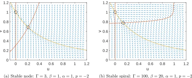
(a) Stable node: Γ = 3,β= 1, α= 1,p=−2
0 0.2 0.4 0.6 0.8 1 1.2
u
0 0.2 0.4 0.6 0.8 1 1.2
v
(b) Stable spiral: Γ = 100,β= 20,α= 1,p=−2
Figure 2.3: Two cases for the phase planes of the spatially homogeneous system for p <0. Steady states are indicated by circular markers.
We are interested in knowing which parameter regimes yield a stable node versus a stable spiral in order to be able to distinguish when we are dealing with cases one and two mentioned above. By using a very small negativep value (α= 1 still fixed), we see that inΓ, β-space, a region around the valueΓ = 4 appears in which the steady state(u∗, v∗)is a stable spiral. Outside of this region, the non-trivial steady state is instead a stable node. An example of these two regions inΓ, β parameter space are shown in Figure 2.4.
Figure 2.4: Separation ofΓ, β-space forp=−0.001 andα= 1for the spatially homogeneous system. The different regions indicate different classifications of the non-trivial steady state (u∗, v∗) as either a stable spiral or a stable node.
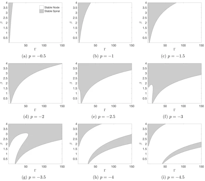
tongue in the stable node region as shown in Figure 2.5. This tongue continues to increase in size, but we never see the disappearance of the stable spiral region. Forplarge and negative, steady state (u∗, v∗) = (ε, v∗) or(u∗, v∗) = (u∗, ε)for someε >0andε <<1. Upon analysis of (2.2), we see that there existsΓ and β sufficiently large to result in ∆(u∗, v∗)<0, and the stable spiral region never completely disappears.
(a)p=−0.5 (b)p=−1 (c) p=−1.5
(d)p=−2 (e)p=−2.5 (f)p=−3
(g)p=−3.5 (h)p=−4 (i)p=−4.5
Figure 2.5: Classification of steady state(u∗, v∗) for increasingly negative values ofp inΓ, β-space with α = 1. The gray area indicates the values of Γ andβ which yield a stable spiral at (u∗, v∗), while the white area indicates values yielding a stable node.
Theorem 2.2.1. For system 2.1 withp <0, the steady state(u∗, v∗) is globally stable in the open first quadrant.
Proof. The system given by 2.1, u˙ =f(u) is a continuously differentiable vector field defined over the simply-connected region u, v >0. We chooseH(u, v) = 1/uv. Then
∇ ·(Hu˙) = ∂
∂u(Hu) +˙ ∂ ∂v(Hv)˙ = ∂
∂u
Γ(1−u) v(1 +e−β(v−α)) −
1 v
+ ∂
∂v
− 1
u(1 +u)p +
1 uv
=− Γ
v(1 +e−β(v−α)) − 1 uv2 <0.
By Dulac’s Criterion, since∇ ·(Hu˙)<0 foru, v >0, there are no closed orbits lying in this region, indicating that(u∗, v∗) is globally stable with respect to system (2.1).
2.3 Phase Plane Analysis: p >0 Case
For p >0, we again begin with an analysis of the non-trivial steady state. The results presented in Section 2.1.1 concerning the trivial steady state still hold forp >0. With a positivep-value, the nullclinev= (1 +u)p becomes monotone increasing, which means that multiple non-trivial steady states are possible. We again fix α = 1 and use a combination of analysis and the continuation software AUTO [28] to find regions within Γ, β-space in which there exist different numbers of non-trivial steady states (for examples of AUTO codes, see Appendix A.1).
Remark 2.3.1. Since u and v are considered physical quantities that must by nonnegative, we are only interested in non-trivial steady states(u∗, v∗) with u∗, v∗ >0.
Using AUTO, we find there exists a pair of curves Γ1(β) and Γ2(β) (for p > 1), which split the parameter space into regions with differing numbers of non-trivial steady states. We define β1 = Γ−11(2) andβ2= Γ2−1(2)and have the following cases for p >0and α= 1:
Case 1: There exists only onesteady state at the trivial location of (0,1)if (a) 1<Γ<Γ1(β)and β > β1.
Case 2: There existtwosteady states, the trivial location (0,1) and a non-trivial location(u∗, v∗), if
(a) Γ = Γ1(β)or Γ = 2 andβ > β1. (b) Γ>2for p≤3.
(c) Γ>Γ2(β)for β1 < β < β2 and p >3.
(d) Γ>2and Γ>Γ2(β) orΓ≤Γ1(β) for β < β1 andp >3. Case 3: There existthree steady states, one trivial and two non-trivial, if
(a) Γ1(β)<Γ<2for β > β1
(b) Γ = 2for β1 < β < β2 and p >3. (c) Γ = Γ2(β)for β < β2 and p >3.
Case 4: There existfour steady states, one trivial and three non-trivial, if (a) 2<Γ<Γ2(β)for β1 < β < β2 and p >3.
(b) Γ1(β)<Γ<Γ2(β)for β < β1 and p >3.
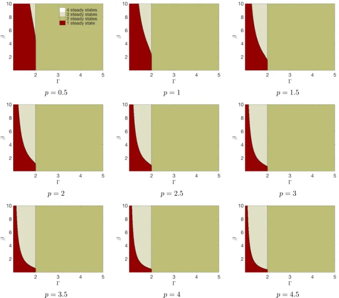
Figure 2.6 displays these four cases inΓ, β-space for increasing values of positivep. Since the region of the parameter space which allows for four steady states is quite small, Figure 2.7 shows this region in greater detail.
We are able to confirm the existence of the boundary curves in Γ, β-space shown in Figure 2.6 for p= 1, 2, 3,and 4 by using an analytical method, which is discussed in greater detail in Appendix B.1. Using this method and the results from the AUTO runs, we can see that the four steady state region ofΓ, β-space does not exist for p= 3and does exist forp= 4. Using AUTO, we can find this region forp-values as small asp= 3.05. This leads us to conjecture that the four steady state region appears forp >3.
For the non-trivial steady state (u, v) = (u∗, v∗), the partial derivatives of f andggiven by (2.3) have the following sign designations forp >0:
p= 0.5 p= 1 p= 1.5
p= 2 p= 2.5 p= 3
p= 3.5 p= 4 p= 4.5
Figure 2.6: The separation of Γ, β-space into regions with different numbers of steady states for p >0 andα= 1.
We see that the discriminant of (2.2)∆(u∗, v∗) = [fu(u∗, v∗) +gv(u∗, v∗)]2−4[fu(u∗, v∗)gv(u∗, v∗)−
fv(u∗, v∗)gu(u∗, v∗)] >0. Therefore the classification of steady state (u∗, v∗) is dependent on the
value offu(u∗, v∗)gv(u∗, v∗)−fv(u∗, v∗)gu(u∗, v∗), and we have the results outlined below forp >0
and α= 1.
Case 1: If fu(u∗, v∗)gv(u∗, v∗)−fv(u∗, v∗)gu(u∗, v∗) <0, then the eigenvalues given by (2.2) are
λ1 >0 andλ2 <0, so (u∗, v∗)is a saddle point.
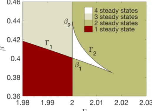
Case 2: If fu(u∗, v∗)gv(u∗, v∗)−fv(u∗, v∗)gu(u∗, v∗) >0, then λ1, λ2 < 0, so (u∗, v∗) is a stable
Figure 2.7: The region in Γ, β-space which yields four steady states for p = 4.5 andα = 1. The curves Γ1(β),Γ2(β) are labeled as well as their respective intersections withΓ = 2,β1 and β2.
Case 3: Iffu(u∗, v∗)gv(u∗, v∗)−fv(u∗, v∗)gu(u∗, v∗) = 0, then we have a borderline case in which
λ1 <0 andλ2= 0, so the steady state is part of aline of isolated fixed points for the linearized system, and we cannot determine the classification of the steady state for the nonlinear ODE.
Applying these classifications to our four cases for steady states, we have the following designations.
Case 1: If the system hasone steady state, it is located at(0,1)and is a saddle point.
Case 2: If the system has two steady states, (0,1)may be a saddle point, a stable node, or may be a borderline case. The non-trivial steady state (u∗, v∗) is a stable nodeor a borderline caseas well.
Case 3: If the system hasthree steady states,(0,1) is astable node,(u∗1, v1∗) is asaddle point, and(u∗2, v2∗) is astable nodewithu∗1 < u∗2.
Case 4: If the system hasfour steady states,(0,1)is asaddle point,(u∗1, v∗1) is astable node, (u∗2, v∗2) is a saddle point, and (u∗3, v3∗) is astable node withu∗1 < u∗2 < u∗3.
0 0.2 0.4 0.6 u
0 0.5 1 1.5 2 2.5 3
v
(a) Γ = 2.5, β = 3, α = 1,
p= 2
-0.1 0 0.1 0.2 0.3 0.4 0.5 u
1 1.5 2
v
(b) Γ = 1.75, β = 3, α= 1,
p= 2
-0.1 0 0.1 0.2 0.3
u 0.5
1 1.5 2 2.5 3 3.5
v
(c)Γ = 2.0026, β = 0.4021,
α= 1,p= 4.5
Figure 2.8: Three cases for the phase planes of the spatially homogeneous system for p >0. Steady states are indicated by circular markers.
A summary of the pertinent results forp >0is provided in Table 2.3. The table omits borderline cases for simplicity of classification and the one steady state case, which will not result in traveling fronts for the system of partial differential equations.
Γ>2,p≤3ORΓ>2, p >3, β <Γ−11(Γ), or β >Γ−21(Γ)
There aretwosteady states: (0,1)is asaddle pointwith eigenvalues λ1 > 0, λ2 < 0, and (u∗, v∗) is a stable node with λ1, λ2 < 0 and distinct.
Γ1(β)<Γ<2
There arethreesteady states: (0,1)is astable nodewith eigenvalues λ1, λ2 < 0 and distinct; (u∗1, v1∗) is a saddle pointwith λ1 >0 and λ2 <0; (u∗2, v∗2) is astable nodewithλ1, λ2 <0and distinct. For the non-trivial steady states, we haveu∗1< u∗2.
Γ>2, p >3, and Γ−11(Γ)< β <Γ−21(Γ)
There arefoursteady states: (0,1)is asaddle pointwith eigenvalues λ1 >0, λ2<0;(u∗1, v1∗) is astable node with λ1, λ2 <0and distinct; (u∗2, v∗2) is asaddle pointwithλ1>0andλ2 <0; (u∗3, v∗3) is astable node with λ1, λ2 <0 and distinct. For the non-trivial steady states, we have u∗1 < u∗2 < u∗3.
CHAPTER 3
Numerical Approximations of Traveling Wave Solutions
We wish to understand the effect that the parameters Γ, β, α, andp have on the characteristics of the traveling wave solutions. As discussed at the end of Chapter 1, we also have good reason to expect to see traveling wave solutions from the numerical approximations of our system. Numerical experiments support this theory, yielding traveling wave solutions, u(z)ˆ and v(z), with differentˆ behaviors resulting from different parameter sets. The different types of traveling waves we observed and their unique characteristics will be described in this chapter.
3.1 Numerical Approximation Methods
The traveling wave profiles we present in this chapter are approximated and verified through two separate methods. In the first method, we use a first order upwind scheme to approximate the time derivative and a second order central difference to approximate the second derivative with respect tox in (1.2). We solve this discretized system over a finite domain with zero Neumann boundary conditions and various initial conditions. So, for the following problem:
ut=d1uxx+f(u, v),
vt=d2vxx+g(u, v), ∂u
∂x(0, t) = 0, ∂v
∂x(0, t) = 0, ∂u
∂x(L, t) = 0, ∂v
∂x(L, t) = 0,
we use the discretized scheme:
uk+1= d1∆t (∆x)2Au
k+ ∆tf(u,v),
vk+1= d2∆t (∆x)2Bv
wherek represents the number of time steps,∆trepresents the size of each time step,∆xrepresents the size of each discretized element of space,uk andvk represent a vectors of u andv defined at each discretized point of space at time stepk,
A=
−2 +(∆d x)2
1∆t 2 0 . . . 0
1 −2 +(∆d x)2
1∆t 1 . . . 0
. ..
0 . . . 1 −2 +(∆dx)2
1∆t 1
0 . . . 0 2 −2 +(∆dx)2
1∆t ,
andB is an identical matrix whered1 is replaced by d2. For initial conditions, we used a variety of decreasing exponentials foru. For example, we usedu(x,0) =Ce−bx with varying values ofC >0 and b >0and also used u(x,0) =Cδ(x) to represent a decreasing exponential withb→ ∞. Forv, we used a constant function, v(x,0) =D, where we require that Dis greater than the critical social tensionα in order to start the system in an excited (rioting) state.
In the second method, we use a version of the algorithm described in [29] and [30]. We first assume solutions of the form u(x, t) = ˆu(x−ct) andv(x, t) = ˆv(x−ct), wherez=x−ct, for (1.2). This results in the system:
d1uˆ00(z) +cˆu0(z) +f(ˆu,ˆv) = 0, d2vˆ00(z) +cˆv0(z) +g(ˆu,ˆv) = 0, ˆ
u(+∞) = 0,ˆv(+∞) = 1,u(−∞) =ˆ u∗,ˆv(−∞) =v∗,
(3.1)
mentioned at the end of Chapter 1, where (u, v) = (0,1) and (u, v) = (u∗, v∗) are the respective trivial and non-trivial stationary points of the system. We then write (3.1) as a system of first order ODEs:
ˆ
u0 = ˆ u ˆ v w y 0 = w y −1
d1(cw+f(ˆu,ˆv)) −1
d2(cy+g(ˆu,v))ˆ
with asymptotic boundary conditions:
(ˆu,ˆv, w, y)→(0,1,0,0) as z→+∞, (ˆu,v, w, y)ˆ →(u∗, v∗,0,0) as z→ −∞.
For simplicity, we letuˆ = [ˆu v w y]ˆ T, uˆ+= [0 1 0 0]T, and uˆ−= [u∗ v∗ 0 0]T. Numerically, we
can only solve the problem above for a finite domain, so we need to find an appropriate replacement for the boundary conditions at positive and negative infinity. We employ the following projective boundary conditions for a finite domain ofz∈[−L, L]:
Ps(ˆu−)(ˆu(−L)−uˆ−) = 0 and Pu(ˆu+)(ˆu(L)−uˆ+) = 0, (3.3)
where Ps(ˆu
−) is a matrix whose rows form a basis for the stable eigenspace of the transpose of the
Jacobian off(ˆu−) andPu(ˆu+) is a matrix whose rows form a basis for the unstable eigenspace of the transpose of the Jacobian off(ˆu+).
These projective boundary conditions alone are not enough to solve system (3.2). Because of the translational invariance of traveling wave solutions, we must impose an extra condition to guarantee the uniqueness of our solution. Instead of the integral condition suggested in [29], we follow a method similar to that presented in [30] and split the domain [−L, L] in half, using a transformation to reflect the left half of the domain to the right. This results in solving the following eight-dimensional system over the domain z∈[0, L]
ˆ
u
ˆ
u1 =
f(ˆu) −f(ˆu1)
conditions may need to be made (for example, the use of wave speed, c, as a free parameter if the system is over-determined).
Besides the utility of having two methods to double check results, the time evolution method and the boundary value solver have their respective advantages. Using the time evolution method, we can observe the development of the traveling wave, and we can see if the initial conditions have an effect on the solutions (specifically the wave speed). The boundary value solver can simultaneously solve for the wave speed in certain cases, and we are also able to find profiles for unstable waves. This is not possible using the time evolution method. The MATLAB code for each of these respective methods is provided in Appendix A.3. The second method utilizes the MATLAB boundary value problem solverbvp5c as well as some of the functions from the STABLAB library. The STABLAB functions have been altered slightly to allow the classification ofc as a free parameter. The altered versions of these functions are given in Appendix A.3 as well.
3.2 Results from Numerical Simulations
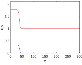
Numerical results from the two methods show that there is a clear division in the characteristics of the traveling wave solutions depending on the values of the parameters Γ,β, α, andp. One of the characteristics that changes quite clearly depending on these values is the monotonicity of the traveling waves. For p >0, we observe only monotone waves. Two examples of these waves are shown in Figure 3.1.
0 50 100 150 200 250 300
x
0 0.5 1 1.5 2
u,v
u(x,t) v(x,t)
(a) Monostable, two steady state case with Γ = 100,β= 5,α= 1, andp= 1.
0 50 100 150 200 250 300
x
0 0.5 1 1.5 2
u,v
(b) Bistable, three steady state case with Γ = 1.5,β = 10,α= 1, and p= 2.
These two profiles are results of the time evolution method. The profile on the left results from the two steady state (monostable) case discussed in Section 2.3, while the profile on the right is the product of a three steady state (bistable) case.
Remark 3.2.1. Using the time evolution method, we were unable to find a traveling wave for the four steady state case for p >0. However, using the boundary value solver, we were able to find a front connecting the two stable steady states as shown in Figure 3.2.
-50 0 50
x 0
0.5 1 1.5 2 2.5 3 3.5
u, v
u(x,t) v(x,t)
Figure 3.2: Traveling wave profile for solutions u(x, t) andv(x, t)for p >0: bistable case with four steady states andΓ = 2.0026,β= 0.4021,p= 4.5, andα = 1.
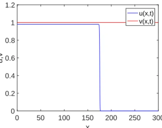
For p = 0, we observe a monotone wave for u(x, t) and a constant solution of v(x, t) = 1(see Figure 3.3). Since we have not observed non-monotone or oscillatory waves for eitherp >0 orp= 0, we have not seen the traveling peak of high intensity rioting behavior, and if we wish to model a riot in which more than one wave of increased rioting behavior is present, we require more than one triggering event.
0 50 100 150 200 250 300
x 0
0.2 0.4 0.6 0.8 1 1.2
u,v
u(x,t) v(x,t)
For p <0, we observe both monotone and non-monotone waves depending on the value of the remaining parameters: Γ, β, and α. Within the group of non-monotone waves, there exists a further distinction. We observe solutions in which the traveling wave u(z) is non-monotone and v(z) is monotone as in the case presented in Figure 3.4a, and we observe solutions in which bothu(z) and v(z)are oscillatory as shown in Figure 3.4b. Keeping the application of our system in mind, we note that these non-monotone waves indicate fluctuations in rioting behavior and social tension.
Remark 3.2.2. It is interesting that the oscillatory wave exhibits a kind of “aftershock” behavior: there is an initial peak of maximum rioting behavior, followed by a sharp decrease in activity and then several more peaks of decreasing magnitude follow. This behavior has only been observed for parameter sets in which the value of β is significantly greater, meaning that these fluctuations are only seen when the transition from a peaceful state to a rioting state is very fast.
0 50 100 150 200 250 300
x
0 0.2 0.4 0.6 0.8 1 1.2
u,v
u(x,t) v(x,t)
(a) Example of a non-monotone wave with Γ = 100,β= 2,α= 1, andp=−2.
0 50 100 150 200 250 300
x
0 0.2 0.4 0.6 0.8 1 1.2
u,v
(b) Example of an oscillatory wave with Γ = 100, β= 20,α= 1, andp=−2.
Figure 3.4: Traveling wave profiles for solutionsu(x, t) andv(x, t) for p <0.
3.3 Numerical Approximation of Wave Speed
For certain numerical computations, it is necessary to have an numerical approximation of the wave speed of the traveling wave solution after it has reached a consistent profile, and we would like to be able to see how the initial conditions of our system affect the wave speed. For the time evolution method, we also want to ensure that the domain is large enough to allow the traveling wave to reach a steady state in which its profile is consistent and no longer changing.
domain in the time evolution method. Each time a buoy is lifted by the wave profile above a threshold height, the wave speed is calculated using the difference in horizontal distance from the previous buoy and the time that passes as the wave travels between the two buoys. A sample profile with buoy markers is shown in Figure 3.5.
0 100 200 300 400 500 600 700
x
0 0.2 0.4 0.6 0.8 1
u(x,t)
u(x,t) Buoy
Figure 3.5: A numerically-approximated solution profile for the Fisher-KPP equation with buoys shown.
We assume the wave has reached a consistent steady state once the calculated wave speed remains within of itself over a fraction of the total domain. For example, for the wave speed experiments presented later in this section, we useε= 0.0005and a fraction of 0.15 of a total domain length of 500. For these numbers, an approximate wave speed value would be reported by the program once the calculated wave speed values were consistent to three decimal places over a domain length of 75. The fraction of the domain and epsilon value are arbitrary and depend on the desired accuracy. The fraction of the domain can be increased or the value can be decreased to achieve greater accuracy for the wave speed approximation.
To test this method, we use two instances of the Fisher-KPP equation [13] and several results known to be true about the wave speed. For the special wave speedc= 5√6 and using the change of variables to a moving frame of reference z =x−ct, the Fisher-KPP equation has the explicit solutionu(z) = 1
(1+Cez/√6)2 forC >0[19]. It is also known that for initial datau(x,0) =Ce
−kx, the
traveling wave solution to the Fisher-KPP equation has wave speedc= 2fork≥1 andc=k+k1 for k <1[20, 21, 22, 23, 24].
method described to find the wave speed of the traveling wave solution for the Fisher-KPP equation with the following initial data:
ut=uxx+u(1−u) ∂u
∂x(0, t) = 0, ∂u
∂x(L, t) = 0,
u(x,0) = 1 (1+ex/√6)2,
(3.4) and
ut=uxx+u(1−u) ∂u
∂x(0, t) = 0, ∂u
∂x(L, t) = 0,
u(x,0) =e−x.
(3.5)
For (3.4), we found a wave speed of c≈2.04081. Compared to the expected wave speed ofc= √5
6, this approximation has an absolute error of 4.25×10⁻⁴. For (3.5), we found a wave speed of c≈1.99740and compared to the expected wave speed of c= 2, this approximation has an absolute error of3.6×10−3.
We can use this method to approximate wave speeds for the monostable and bistable cases. For the bistable case, we may also use boundary value solver with wave speed set as a free parameter as mentioned in the previous section. The MATLAB code for the wave speed approximation method mentioned in this section is provided in Appendix A.3.
3.3.1 Wave Speed Experiments
Since our p = 0case reduces to a Fisher-KPP equation, we can use the theory to check that there are similar conditions for the wave speed of the traveling wave solutions. We expect that there exists some cmin= 2
p
d1fu(0,1)such that forc < cmin there exists no traveling wave, and we also
expect to see a dependence on initial conditions of the formu(x,0) =Ce−kx, where c=cmin for
k ≥p
fu(0,1)/d1 and c = d1k+fu(0,1)/k for k <
p
fu(0,1)/d1 [14, 20, 21, 22, 23, 31, 25]. We wish to make some preliminary observations of the wave speed of the numerically-approximated solutions to the system under different parameter values to see if the behavior for p= 0 appears numerically to hold for other values ofp.
no effect on the minimum wave speed for the traveling wave solutions for p = 0. We test this hypothesis for various values ofΓ, specifically values that should yield a whole number wave speed forcmin = 2
p
d1fu(0,1). We letd1, d2= 1, and test values ofΓ = 10,52, and 100,β= 1,5, 10, and
50, and p= 2,1,0,−1, and −2. The results of these runs are shown in Tables 3.1 through 3.5.
β
1 5 10 50
Γ
10 3.9904 3.9904 3.9904 4.3507 52 9.9354 9.9354 9.9354 9.9354 100 13.8408 13.8408 13.8318 13.8408
Table 3.1: Approximate minimum wave speed,cmin, values forp= 2.
β
1 5 10 50
Γ
10 3.9904 3.9904 3.9904 4.1314 52 9.9354 9.9354 9.9354 9.9354 100 13.8408 13.8408 13.8408 13.8313
Table 3.2: Approximate minimum wave speed,cmin, values forp= 1.
β
1 5 10 50 Expected
Γ
10 3.9904 3.9904 3.9904 3.9888 4 52 9.9354 9.9354 9.9354 9.9354 10 100 13.8408 13.8408 13.8408 13.8313 14
Table 3.3: Approximate minimum wave speed, cmin, values for p = 0. The expected wave speed
values are calculated usingcmin= 2
p
d1fu(0,1).
β
1 5 10 50
Γ
10 3.9904 3.9904 3.9904 3.9853 52 9.9354 9.9354 9.9354 9.8736 100 13.8408 13.8408 13.8408 13.6612
β
1 5 10 50
Γ
10 3.9904 3.9904 3.9904 3.9853 52 9.9354 9.9354 9.9354 9.8736 100 13.8408 13.8408 13.8313 13.6612
Table 3.5: Approximate minimum wave speed,cmin, values forp=−2.
We can see that from table to table, there is very little discrepancy in the minimum wave speed values except in the case of β = 50 and p > 0. In these cases, we can see significantly higher approximate wave speed values (see Tables 3.1 and 3.2). It is possible that these differences are due to numerical error, or it could be the case that the minimum wave speed actually does have some dependence onβ andp. Based on the p <0data, we support the former theory since we do not see a corresponding significant change in the wave speed values for p <0, and this difference does not appear for larger values of Γ. Also, we would expect to see deviations in the wave speed forp <0 rather thanp >0 because forp≥0, the system is monotone. For the valuesΓ = 10,52, and 100 andp= 0, we would expect to see wave speed values of cmin = 4,10, and 14, respectively (see note
in Table 3.3). The values in the tables are very close although we do see a decrease in accuracy for largerΓ. We think that this is simply a function of using the same accuracy and domain restrictions for each of these runs and that because of the size of the parameter, it may be necessary to make these restrictions more stringent (run the experiment over a larger domain and require speeds to be within a smallerεvalue of each other) for larger values of Γ. This idea is supported by the fact that we also see a loss of accuracy for our expected values of wave speed for large values of β for the runs.
After seeing that we get greater expected accuracy in approximated wave speed for smaller values ofΓ andβ and seeing that there is little variation between speeds for different values ofp, we decide to test the dependence of wave speed on initial conditions, using an initial condition of u(x,0) = 5e−kx withk=−.25, 0.5, 1, 1.5, and 2 forp= 2,1, 0,−1, and −2,Γ = 10, and β = 1. We choose smaller values ofΓ andβ to hopefully get more accurate approximations. The results of these runs are shown in Table 3.6.
k
0.25 0.5 1 1.5 2
p
2 16.2338 8.4692 4.9975 4.1641 3.9944 1 16.2338 8.4692 4.9975 4.1641 3.9944 0 16.2338 8.4692 4.9975 4.1641 3.9944 −1 16.2338 8.4692 4.9975 4.1641 3.9944 −2 16.2338 8.4692 4.9975 4.1641 3.9944 Expected* 16.25 8.5 5 4.1667 4
Table 3.6: Approximate wave speed,c, values for runs with initial conditionsu(x,0) = 5e−kx,Γ = 10, β = 1. *Expected values are only intended for the casep= 0, where we have calculated the values using c=d1k+fu(0,1)/k.
CHAPTER 4
Existence of Traveling Wave Solutions
This chapter is devoted to the existence of traveling wave solutions forp≥0. 4.1 Background
For the system:
ut=Auxx+F(u), (4.1)
where
A=
d1 0 0 d2
and F(u) =
f(u, v) g(u, v)
, (4.2)
there is a traveling wave solution to (4.1) if there is a solutionu(x, t) = ˆu(x−ct), wherez=x−ct for some c∈Rthat satisfies the system
Aˆu00+Cuˆ0+F(u) = 0 (4.3)
and the limits
lim
z→±∞uˆ(z) = ˆu±, (4.4)
whereA is defined as in (4.2) and
C=
c 0 0 c
.
When the parameterp≥0, system (4.1) ismonotone, or order-preserving, meaning that
∂Fi
∂uj
≥0, for i, j∈1,2, i6=j, (4.5)
For the corresponding spatially homogeneous system of (4.1):
d
dt(u) =F(u),
we call the source bistable if the stationary points,uˆ±are both stable. We call the sourcemonostable
if one of the stationary points (eitheruˆ+ oruˆ−) is unstable.
Much work has been done concerning the existence of traveling waves in monotone systems, and we utilize the several theorems to prove the existence of traveling wave solutions [14, 18, 32, 26, 33]. For the remainder of this document, we will use DF(u) to denote the Jacobian of F(u).
Theorem 4.1.1. Existence of traveling wave solution for system with bistable source: Assume that system (4.1) is monotone and thatF(ˆu+) =F(ˆu−) = 0, whereuˆ+<uˆ−. Suppose also that F(u)
vanishes at a finite number of points uk, with uˆ+≤uk≤uˆ− (k= 1, ..., m). Let us assume that all
eigenvalues of the matricesDF(ˆu±) lie in the left half-plane and that there exist vectorsqk ≥0 such
that qkDF(uk) >0, k = 1, ..., m. Then there exists a unique monotone traveling wave: a unique
constantc (the wave speed) and a unique twice continuously differentiable monotone vector-valued function uˆ(z) that is monotonically decreasing and satisfies system (4.3) and the limits given in (4.4).
Theorem 4.1.2. Existence of traveling wave solution for system with monostable source: Assume that system (4.1) is monotone and that F(ˆu+) =F(ˆu−) = 0, where uˆ+ <uˆ−. Suppose also that
F(u) vanishes at a finite number of pointsuk, withuˆ+≤uk≤uˆ−(k= 1, ..., m). Let us assume that
all eigenvalues of the matrices DF(ˆu−)lie in the left half-plane and that matrices DF(ˆu+), DF(uk)
with k= 1, ..., m, have eigenvalues in the right half plane. Then there exists a positive constant cmin
such that for all c≥cmin there exist monotone waves satisfying system (4.3) and the limits given in
(4.4). Whenc < cmin, such waves do not exist.
Remark 4.1.1. We note that forp <0, our system is not monotone since gu(u, v)<0 foru, v >0,
4.2 Casep≥0
Forp≥0, we can see that our system (1.2) is monotone. As discussed in Sections 2.1 and 2.3, for p= 0, the spatially homogeneous system given in (2.1) has a monostable source. In other words, it has two stationary points, one of which is stable and the other unstable. Forp >0, we are interested in the cases in which the spatially homogeneous system has two, three, or four stationary points. When there are only two stationary points, the system has a monostable source, but the system is bistable when there are three or four stationary points.
4.2.1 Bistable Case
We consider system (4.1) with F(u) defined as in Section 1.2.
Theorem 4.2.1. For system (4.1), with the following parameters, p >0,Γ1(β)<Γ<2 (i.e., the three stationary point case): there exists a unique monotone, vector-valued traveling waveuˆ(z)that is monotonically decreasing, satisfies system (4.3) and the limits (4.4) and has a unique wave speed,c.
Proof. As mentioned above, for p ≥ 0, our system is monotone. Section 2.3 classified the three stationary point case described above as a bistable case. In other words, we have stationary points ˆ
u+ <u1 <uˆ− for which the eigenvalues ofDF(ˆu+) andDF(ˆu−) lie in the left half-plane. In order
to apply Theorem 4.1.1 to prove existence of a traveling wave, we only need to prove that there exists a nonnegative vector q1= [q1 q2]such thatq1DF(u1) >0. Here we use u1 = [u1 v1]. We see that in order for this to be true, we need
−q1|fu(u1, v1)|+q2|gu(u1, v1)|>0
q1|fv(u1, v1)| −q2|gv(u1, v1)|>0,
where we have used the fact that fu(u1, v1) <0 andgv(u1, v1)<0. Rearranging the inequalities above, we need
q2 > q1|fu(u1, v1)| |gu(u1, v1)|
and q2< q1|fv(u1, v1)| |gv(u1, v1)|
,
and see that there existq1, q2 ≥0 that satisfy these inequalities when |fv(u1, v1)|
|gv(u1, v1)|
or equivalently,
|fu(u1, v1)||gv(u1, v1)| − |fv(u1, v1)||gu(u1, v1)|<0.
Because the interior stationary point u1 is a saddle point for both cases, the inequality above is already satisfied. We see that all the conditions for Theorem 4.1.1 are met, and so there exists a unique, monotone traveling wave solution for the three stationary point case for p >0.
Remark 4.2.1. In the four stationary point case, we have a bistable case because for the stationary points, (u0<uˆ+<u1 <uˆ−), DF(ˆu+) and DF(ˆu−) both have all negative eigenvalues. However,
we are unable to apply the existence theorem for bistable sources (Theorem 4.1.1) because of the trivial, unstable steady state existing outside of the interval created by the two stable steady states. We were, however, able to find traveling front solutions between the two stable stationary points
using the bvp5c method discussed in Chapter 3. Running the numerical time evolution with decaying exponential initial conditions did not yield any such waves. We also attempted using the solution profile from the boundary value solver as an initial condition for the time evolution method, and this did not yield a traveling wave solution either. This seems to indicate that while a traveling front may exist between the two stable states, the wave is not asymptotically stable.
4.2.2 Monostable Case
For the monostable sources, we turn our attention to the case whenp= 0, and whenp >0 with two stationary points. Again, we can take advantage of the monotonicity of our system.
Theorem 4.2.2. For system (4.1), with the following parameters: 1) p >0, Γ >2, or 2) p= 0, Γ>2, there exist two stationary point cases. For these cases, there exists a positive constant cmin
such that for c≥cmin there exist monotone waves satisfying system (4.3) and the limits (4.4). For
c < cmin, no such waves exist.
Proof. As mentioned above, we have a monotone system forp ≥0. For the case in which p = 0 andΓ>2, there are two stationary points,uˆ+<uˆ−. As shown in Section 2.1, the eigenvalues of
DF(ˆu−)all lie in the left half plane, andDF(ˆu+)has one eigenvalue in the right half plane. We can immediately apply Theorem 4.1.2 since every condition is met, so there exists a monotone traveling wave for p= 0 andΓ>2.
the stationary point as outlined in Section 2.3. That is for the parameter sets: 1)Γ>2, p≤3, and 2)Γ>2, p >3, andΓ−11(Γ)< β <Γ−21(Γ), there are two stationary points,uˆ+<uˆ− for which the
eigenvalues ofDF(ˆu−)all lie in the left half plane, andDF(ˆu+) has one eigenvalue in the right half
CHAPTER 5
Asymptotic Behavior of Traveling Wave Solutions
To help prove the stability of the traveling wave solutions later in Chapter 6, we wish to show that for p ≥ 0, the traveling wave solutions approach their asymptotic rest states exponentially quickly. This also allows us to place bounds on our solutions. To accomplish this, we will utilize a method similar to one presented in [35, 36]. We linearize our system about the traveling wave solution and then look for the asymptotic behavior of the solutions to the linearized system. This will give asymptotic decay rates for the traveling wave solution. For simplicity, we assumed1=d2 = 1 in (1.2). This generalization is trivial. Assuming the system has traveling wave solutions u(z)ˆ and ˆ
v(z), the moving coordinate system z=x−ct may be used with ut=vt= 0, yielding the following
new system:
−cuz=uzz+f(u, v),
−cvz =vzz+g(u, v),
which can be represented as a first order, four dimensional system of equations:
u0 =w, v0=y,
w0 =−cw−f(u, v), y0=−cy−g(u, v).
(5.1)
As mentioned before, this system has non-trivial steady states (u∗, v∗,0,0)withu∗, v∗ >0 and trivial state (0,1,0,0), where in most cases u∗ andv∗ must be numerically calculated and satisfy the equations
0 = Γ(1−u
∗)
1 +e−β(v∗−α) −1 and 0 =− v∗
(1 +u∗)p + 1. (5.2)
steady states(u∗, v∗,0,0)satisfying (5.2).
The linearization of (5.1) about the steady states is given by U0 =AU:
U0 = u v w y 0 =
0 0 1 0
0 0 0 1
−fu(u, v) −fv(u, v) −c 0
−gu(u, v) −gv(u, v) 0 −c
u v w y
=AU, (5.3)
whereA can be evaluated separately at each of the respective steady states. The eigenvalues,λ, of A are given by
[λ(c+λ)]2+ [λ(c+λ)][fu(u, v) +gv(u, v)] +fu(u, v)gv(u, v)−gu(u, v)fv(u, v) = 0.
Using the substitutionµ=λ(c+λ)in the equation above, we have the following values for µ:
µ1,2=
−[fu(u, v) +gv(u, v)]
2 ±p
[fu(u, v) +gv(u, v)]2−4[fu(u, v)gv(u, v)−gu(u, v)fv(u, v)]
2 .
(5.4)
The eigenvalues of Aare then given by the solutions toλ(c+λ) =µ1 andλ(c+λ) =µ2:
λ1,2 =
−c±pc2+ 4µ 1
2 , λ3,4 =
−c±pc2+ 4µ 2
2 . (5.5)
We then use these eigenvalues to determine the asymptotic decay rates of the linearized system (5.3) forp= 0andp >0. For reference, the partial derivatives off(u, v)andg(u, v) are again given
below:
fu(u, v) =
Γ(1−2u)
1 +e−β(v−α) −1, fv(u, v) =
βΓe−β(v−α)u(1−u) (1 +e−β(v−α))2 , gu(u, v) =
pv
5.1 Casep= 0
For p= 0, we assume thatuˆ(z) = [ˆu(z) ˆv(z)]T represents traveling waves satisfying
lim
z→+∞uˆ(z) =
0 1
, z→−∞lim uˆ(z) = u∗ v∗ ˆ
u(z),v(z)ˆ >0, uˆ0(z)<0, ˆv0(z) = 0.
Proposition 5.1.1. [35] Asymptotic decay rates for p= 0:
(a) Let uˆ+= [0 1]T and uˆ−= [u∗ v∗]T. There are nonnegative vectorskc,Kc,Kε,m,M,Mδ and
positive numbers λc, λcmin, µ, µf, ε, δ such that the nonzero elements of Kε,Mδ approach ∞ as
ε, δ→0 and
kce−λcz≤ˆu(z)−uˆ
+≤Kce−λcz, (z≥0), c > cmin ˆ
u(z)−uˆ+≤Kεe−(λcmin−ε)z, (z≥0), c=cmin
meµz≤uˆ−−ˆu(z)≤Meµz, (z≤0), fu(u∗, v∗)6=−1
ˆ
u−−ˆu(z)≤Mδe(µf−δ)z, (z≤0), fu(u∗, v∗) =−1
(b) There are nonpositive vectors hc,Hc,Hε,n,N,Nδ and positive numbersλc, λcmin, λ, µ, µf, ε, δ
such that the nonzero elements of Hε,Nδ approach ∞ as ε, δ→0 and
hce−λcz ≥uˆ0(z)≥Hce−λcz, (z≥0), c > c
min
ˆ
u0(z)≥Hεe−(λcmin−ε)z, (z≥0), c=cmin neµz≥ −ˆu0(z)≥Neµz, (z≤0), f
u(u∗, v∗)6=−1
−ˆu0(z)≥Mδe(µf−δ)z, (z≤0), fu(u∗, v∗) =−1
Proof. Using (5.4) and (5.5), we find the eigenvalues of A|(0,1,0,0) andA|(u∗,v∗,0,0) to help determine asymptotic estimates for the traveling wave solution. The eigenvalues forA|(0,1,0,0) and A|(u∗,v∗,0,0) are, respectively,
A|(0,1,0,0) : λ1,2=
−c±p
c2−4f
u(0,1)
2 , λ3,4 =
−c±√c2+ 4