HIERARCHICAL LOOP STRUCTURES REGULATE CHROMOSOME ORGANIZATION
Yunyan He
A dissertation submitted to faculty at the University of North Carolina at Chapel Hill in partial fulfillment of the requirements for the degree of Doctor of Philosophy in the
Department of Mathematics in the Graduate School.
Chapel Hill 2020
Approved by: M. Gregory Forest Kerry Bloom
David Adalsteinsson Jingfang Huang
ii © 2020 Yunyan He
iii
ABSTRACT
Yunyan He: Hierarchical Loop Structures Regulate Chromosome Organization (Under the direction of M. Gregory Forest, David Adalsteinsson and Kerry Bloom)
The study of chromatin dynamics and motion is essential to the understanding of the
rules of life; indeed, the dynamic organization of chromatin plays a unique role in nearly all
DNA metabolic processes. It has been hypothesized, and heavily explored experimentally,
that various classes of proteins participate in managing the geometrical structure and
dynamics of chromosomes throughout the cell cycle. While histones effectively compact
chromosomes, the extent of compaction (7-fold) does not account for the greater than
1000-fold compaction required to reduce the genome (length ~1 meter) to the size of the nucleus
(radius ~2 micron). It has recently been shown that condensins, one class of structural
maintenance of chromosome (SMC) proteins, are able to extrude loops along the chromatin
fiber, providing a mechanism to further compact the genome. The role of condensins during
mitosis is a potential means for the 10,000-fold compaction attained at the time of
chromosome segregation to daughter cells. Condensin and the loop-extrusion mechanism
may also be responsible for the heterogeneous shape of chromosomes. In this work, a
real-time numerical simulation model is introduced to simulate chromosome dynamics in the
presence of histones and condensins to provide a realistic model based on physical principles
of polymer dynamics and loop formation. We show that chromosome compaction and
variance in compaction result from the coupled hierarchical loop structures created by both
histones and condensins, and not from either individual effect.
To study the existence of sub-nuclear domains in the nucleus, another coarse-grained
iv
replicates the phase separation of the nucleolus, reveals dynamic self-organized clustering of
genes within the nucleolus, and accurately predicts that multiple rDNA loci positioned on
more than one chromosome will behave remarkably similarly to a single, intact nucleolus,
despite varying the geometric positions of the loci. In this work, a new numerical method to
identify the 3D territory is developed to measure the volume of the nucleolus. Simulation
results reveal that the nucleolus gains compaction due to high frequency binding-unbinding
kinetics of dynamic crosslinks, and the multiple-loci nucleolus gains comparable volume with
v
ACKNOWLEDGEMENTS
I would like to thank all of you who helped me or inspired me along the journey of my
years at UNC. The impact on me is valuable and will last for my entire life. Forgive me for
limiting the list to a few.
Dad and mom
Thank you for always supporting me. This has been important to me because you give
me the courage and confidence to lead my life in my own way. I feel really sorry for being far
apart from you for all these years.
Yi
Strange to call you Yi so I will go with Laopo. Thank you for everything, as always. I
can carry on because I know you are by my side. The highlight of the past five years was
definitely the moment you said “yes”.
All my friends at UNC
It has been great fun to develop hobbies with all of you. Basketball, volleyball, video
games, chatting … Let’s continue enjoying our lives in the future, no matter where we are.
My Committee, Jingfang Huang, and Katherine Newhall
Thank you for guiding my research. A lot of your suggestions are valuable and helped
me reexamine my work. I am grateful you agreed to be on my committee.
David
The courses and research projects you helped me with showed me the essence of
programming and actually led my way towards this path. Thank you very much for your help.
vi
I could never image to work with biologists in interdisciplinary study is such a fun
and cool thing. Thank you for showing me a different field of science, and thank you for your
patience and kind help to a biology-free kid to accomplish all these.
Greg
You showed me the strategy to be a great scientist: be vigilant to opportunities and
have big scope. This has inspired me and will always lead me in the future. Thank you so
vii
TABLE OF CONTENTS
LIST OF TABLES ... x
LIST OF FIGURES ... xi
LIST OF ABBREVIATIONS ... xii
CHAPTER 1: CENTROMERIC CHROMOSOME DYNAMICS SIMULATOR BASED ON POLYMER MODEL ... 1
SUMMARY ... 1
INTRODUCTION ... 1
SIMULATION METHODS ... 3
Model Description ... 4
Tensile Stiffness ... 4
Bending Rigidity ... 5
Thermal Fluctuations ... 9
Collision Repelling Force ... 10
Fluid Drag Force ... 12
Equation of Motion ... 12
Stability and Constraints ... 13
Simulation Program ... 14
RESULTS ... 16
Brownian motion validation ... 18
Rouse time ... 18
End-to-end distance ... 19
Radius of gyration ... 19
DISCUSSION ... 24
viii
SUMMARY ... 26
INTRODUCTION ... 26
METHODS ... 29
Histones ... 29
Condensins ... 30
Data analysis methods ... 36
RESULTS ... 37
Experimental Results ... 37
Simulation Results: histones and condensins compact the dicentric plasmid ... 39
DISCUSSION ... 49
CHAPTER 3: HIERARCHICAL CHROMATIN LOOPS REGULATE CHROMOSOMAL STRUCTURE IN VARIOUS WAYS ... 51
SUMMARY ... 51
INTRODUCTION ... 51
Hierarchical loop structures cause condensed yet dynamic chromosome organization ... 53
Hierarchical loop structures affect polymer mobility ... 55
METHODS ... 56
Experimental Methods ... 56
Numerical methods simulating biological mutants ... 61
Simulations varying polymer stiffness and measuring chromosomal mobility. ... 62
RESULTS ... 64
In a condensin-concentrated environment, histone enrichment leads to stable DNA structure ... 64
DNA is condensed under the existence of condensin-mediated loops in dicentric plasmid chromosome ... 70
Tension-dependent extrusion behavior for condensins benefits formation of effective loops. .. 76
Hierarchical loop structures modify chromatin stiffness ... 79
DISCUSSION ... 85
The balance between condensins and histones affects the compaction effect ... 85
ix
Indication of existence of Z-loops ... 87
CHAPTER 4: DYNAMIC CHROMOSOMAL CROSSLINKS CONDENSE AND STABILIZE STRUCTURAL HETEROGENEITY OF THE NUCLEOLUS ... 91
SUMMARY ... 91
INTRODUCTION ... 91
MATERIALS AND METHODS ... 93
Chromosome Modeling Approach ... 93
Nucleolus ... 94
Signal Transformation ... 95
RESULTS ... 96
Yeast nucleus simulation results ... 96
Simulated signal processing results ... 103
Community structure compacts the nucleolus. ... 106
Split nucleolus does not lead to significant volume change in nucleolus ... 107
DISCUSSIONS ... 109
CHAPTER 5: FUTURE DIRECTIONS ... 111
COMPLETION AND EXTENSIONS OF SIMULATIONS ON CHROMATIN DYNAMICS ... 111
APPENDIX 1: CHROMOSOME SIMULATION MANUAL ... 114
x
LIST OF TABLES
Table 1.1: Plasmid chromosome simulation tunable parameters ... 15
Table 1.2: Averaged radius of gyration and end-to-end distance ... 23
xi
LIST OF FIGURES
Figure 1.1: Illustration of hinge force ... 8
Figure 1.2: Simulated free-floating linear polymer chain ... 17
Figure 1.3: End-to-end distance plot of simulated free-floating linear chains ... 21
Figure 1.4: Radius of gyration plot of simulated free-floating linear chains ... 22
Figure 2.1: Illustration of histone model and condensin model ... 34
Figure 2.2: Dicentric plasmid chromosome signal and signal length analyses ... 38
Figure 2.3: Geometry of simulated plasmid chromosome ... 44
Figure 2.4: Signal length analyses of simulated plasmid signals ... 46
Figure 2.5: Tension-related analyses of plasmid chromosome in distinct protein conditions. 48 Figure 3.1: Images of experimental observations in vivo. ... 60
Figure 3.2: Experimental Report on WT vs. SPT10Δ plasmid signals ... 67
Figure 3.3: Report on simulated WT vs. SPT10Δ plasmid signals ... 69
Figure 3.4: Experimental report on WT vs. ycg1-2 plasmid signals ... 73
Figure 3.5: Report on simulated WT vs. ycg1-2 plasmid signals ... 75
Figure 3.6: Comparison plots varying condensins’ tension-dependent extrusion behavior .... 78
Figure 3.7: Varying stiffness lead to unexpected results with hierarchical loop structures .... 81
Figure 3.8: Pairwise contact frequency map of simulated plasmids ... 82
Figure 3.9: Reginal MSD plots for simulated heterogeneous plasmid chromosomes ... 84
Figure 3.10: Graphical demonstration of Z-loop structures ... 90
Figure 4.1: Simulated chromosomes in yeast nucleus ... 100
Figure 4.2: Snapshots of simulated nucleolus beads ... 102
Figure 4.3: Simulated 3D signals of nucleolus ... 104
Figure 4.4: Simulated 2D signals of nucleolus ... 105
xii
LIST OF ABBREVIATIONS
3C – Chromosome Conformation Capture
bp – Base Pair
GFP – Green Fluorescent Protein
kbp – Kilo Base Pairs
lacO – Lactose Operon
𝐿! – Persistence Length
MSD – Mean Squared Displacement
P – Poise
RFP – Red Fluorescent Protein
𝑅" – Radius of Gyration
SMC – Structural Maintenance of Chromosomes
tetO – Tetracycline Operon
WT – Wild Type
1
CHAPTER 1: CENTROMERIC CHROMOSOME DYNAMICS SIMULATOR BASED ON POLYMER MODEL
Summary
The geometrical structure of chromosomes has profound significance in cell biology.
Chromosomes are carriers of DNA and are confined and compacted within the nucleus. The
mechanistic causes for the compactness and orderliness of chromosomes remains to be
explored. In order to learn the physical principles leading to the compact structure, we
construct a mathematical simulation pipeline based on a polymer-physics based model to
simulate the dynamics of chromosomes inside the nucleus of a living cell. The simulation is
numerically stable, and is well-designed for future modifications. The numerical results are
tested against existing results in the field of polymer physics. The primary purpose for
developing this model is to provide the foundation for constructing genuine simulations
involving additional molecular species in the nucleus and provide insights on how
chromosomes are condensed.
Introduction
DNA carries and replicates biological information and is generally accepted as one of
the most important genetic materials in living beings. In eukaryotic cells, DNA forms long,
compact structures called chromosomes. These structures are highly organized and
compacted in the nucleus. There are 23 pairs of chromosomes in each human cell, with a total
arclength of roughly 2 meters. These structures are confined in the nucleus by its membrane,
with a diameter of about 2 𝜇𝑚. It requires significant and active compaction processes to
2
sequencing of nucleotides been a hot topic in cell biology over the past decade, but also the
geometrical and topological structure of chromosomes.
In order to study the higher-order structure of chromosomes, biologists seek methods
to observe the geometry of chromosomes. The most widely utilized methods to observe
chromosomes involve the use of DNA-binding or protein-binding fluorescent markers
(Robinett et al., 1996; Straight et al., 1996). Other methods include chromosome
conformation capture (3C) (Sati & Cavalli, 2017) and super-resolution microscopy (Neice,
2010). However, there are limitations for these methodologies. Clear observation down to the
base pair (bp) scale demands very high resolution, which is not attainable with light
microscopes. Moreover, since chromosomes are crowded and tangled in the cell nuclear
environment, the difficulty of separating chromosomes and conducting subtle observations on
isolated segments arises.
Under this context, it is essential to come up with a numerical simulation pipeline that
accurately captures the dynamics of chromosomes in cell environment. Upon a proper choice
of model, the simulation mimics the dynamics of chromosomes in arbitrarily high resolution.
The time cost is significantly lower compared to the cost of cultivating fluorescently tagged
chromosomes for experimental observation. A direct comparison against biological
observations can be conducted to benchmark the validity of the numerical model. More
importantly, numerical simulations are much simpler and cheaper to test hypotheses, and
make predictions to verify experimentally. This creates the opportunity to gain biological
insights from simulations about various mutants that change either the property of a
chromosome or the environmental factors.
In this work, a specific type of chromosome is studied and simulated: the dicentric
plasmid chromosome. It preserves the following properties: it is a small circular DNA
3
Biology at University of North Carolina at Chapel Hill, Prof. Kerry Bloom’s laboratory is
able to synthesize plasmid chromosomes, embed tetR-GFP bound to a tandem tetO operator
DNA array in the chromosomes at prescribed regions for visualization, and activate the
chromosomes in the nucleus in budding yeast cells. The signals captured in microscopy are
processed through image processing pipelines to obtain statistics for further analyses. In
simulations, the same labeling scheme and image processing pipeline is applied to maintain
the best consistency with experiments: the simulation scale is chosen to match the
synthesized 10 kbp (thousand bp) plasmid chromosome. It obtains circular geometry with
two sites pinned in space to mimic sister centromeres connecting chromosomes to
microtubules during the early stage of mitosis; the fluorescent region of DNA is also
highlighted in simulation for a direct comparison of simulated microscopy signals with
proper transformation to experimentally obtained microscopy signals.
The model is based on the well-defined properties of long-chain polymers in a viscous
environment (Rubinstein & Colby, 2003). We establish our model in reference to existing
models (Josh Lawrimore et al., 2019) and engage proper modifications. An individual
dicentric plasmid chromosome is discretized and simulated as a polymer chain governed by
force laws. In addition, fluid drag is incorporated to account for the fluid environment in
cells, while not accounting for hydrodynamic interactions, called the free-draining
approximation. The choices of force components are subject to polymer physics to guarantee
rationality. To validate our simulation, various statistics from the simulation output are
analyzed and compared to existing results in polymer physics.
Simulation Methods
The simulator was developed in C++ using DataTank as the user interface, which
4
simulated chromosomes in this pellucid graphical interface. The C++ program parses 3D
coordinates of the chromosome into a time series as the output. The output file can be directly
read through DataTank, and DataTank provides built-in tools for visualization and analyses.
An overview of the workflow of the simulation pipeline is provided in Appendix 1. A list of
tunable parameters and the default settings are in Table 1.1.
Model Description
The simulation is based on a discretized bead-spring model in a fluid drag
environment. The total 10 kbp plasmid chromosome is discretized into 386 beads, with each
bead representing roughly 10 nm (33 bp) of DNA. Bead 1 and Bead 139 are pinned in space
in the simulation to simulate tethered, static centromeres in the nucleus. Beads are connected
by springs governed by a linear force law and a bending rigidity law. The persistence length
of DNA is 50 nm, set by an additional hinge force in the simulation that controls rigidity.
Thermodynamic fluctuations influence the motion of all particles, and the range the substrate
explores can be tested as a metric for the intensity of the dynamics and the stiffness of the
polymer chain. For faster simulation, a water environment is adopted in the simulation. The
fluid environment attains a viscosity of 0.01 P (Poise). Given the estimation of nuclear
viscosity to be 141 P, the simulation speeds up the evolution process 14100 times, where 0.15
sec total simulation time is equivalent to approximately 35 min real time.
Tensile Stiffness
Two adjacent beads are connected by a spring governed by a linear spring law. It
resists extension of the polymer chain between two beads. We simulate the extension by the
tensile stiffness of a beam, and thus the equations of stress-versus-strain are used. We do not
5
𝝈 = 𝐸𝝐, (1.1)
𝝈 =𝑭$, (1.2)
𝝐 =𝚫𝑳
'!. (1.3)
The spring force for extension due to tension between two adjacent beads can be calculated
by substituting and rearranging equations (1.1) ~ (1.3).
𝑭𝑺𝒑𝒓𝒊𝒏𝒈= .$'!𝚫𝑳, (1.4)
where 𝐸 refers to the Young’s modulus; 𝐴 = 𝜋𝑟/ corresponds to the the area of the
cross-section of the spring; 𝐿0 is the resting length of the spring. For this model, 𝐿0 = 10 𝑛𝑚
since each bead represents about 10 nm of DNA; 𝐸 = 2 𝐺𝑃𝑎 and 𝑟 = 0.6 𝑛𝑚, consistent
with the plasmid chromosome we use.
Bending Rigidity
Chromosomes have a bending rigidity that is associated with DNA linkers. DNA
linkers are the naked DNA strands linking adjacent nucleosomes (a nucleosome is a
substructure formed by ~150 bp of DNA wrapping around an octet of histone proteins). One
standard metric to describe the rigidity in polymer physics is the persistence length, the
length over which correlations between motion of two individual ends are lost (Rubinstein &
Colby, 2003). Greater persistence length refers to the fact that the motions at two distant
locations are still closely correlated, and thus indicating stiffness over the respective distance
between those locations. The rigidity of our chosen plasmid chromosome is approximated by
that of B-form DNA, which is reported to be 50 nm (Dekker et al., 2001). The entropic
flexibility of DNA is consistent with the worm-like chain model in polymer physics (J F
Marko & Siggia, 1995; John F. Marko & Siggia, 1994) which makes worm-like chain models
a common choice in simulating the dynamics of DNA. However, for our simulation focusing
6
bending rigidity deviates from worm-like chain models. Hence, the worm-like chain model is
not applied in our model.
The bending rigidity for the polymer chain is embedded by applying additional force
at each of the bead, in order to keep the substrate straight (Bloom, 2008). If a deflection
occurs between two connecting springs, a shear bending force is produced at the joint to
eliminate the deflection. The mechanism is achieved by considering the chromatin as an
elastic beam, and then Euler-Bernoulli beam theory is applied.
To simplify the system, instead of solving the Euler-Bernoulli equation, a
coarse-grained model is chosen. Assume an elastic rod of length 2𝑑 attains a load at the center, and
the rod is perfectly stiff on both halves from the middle. The restoring force is then
proportional to the degree of deformation characterized by the angle two halves of the rod
make, 𝜃 (Young et al., 1976).
𝑭𝑯𝒊𝒏𝒈𝒆=
2𝐸𝐼
𝑑/ 𝜃𝒏, (1.5)
where E and n refers to Young’s modulus and the normal vector along the direction between
the corresponding springs, respectively. 𝐼 = 𝜋𝑟3/4 is the moment of the area of the beam
with circular cross section. 𝑑 is chosen to be 𝐿0 in this simulation to achieve 𝐿! of 50 nm
for the polymer. The name “hinge” comes from the hinge-like mechanism the rigidity force is
modeled after. See Figure 1.1 for graphical illustration.
𝑭𝑯𝒊𝒏𝒈𝒆 is applied at every bead where the two connecting springs fail to bend
straight, in the direction pointing inward from the angle the springs form. −𝑭𝑯𝒊𝒏𝒈𝒆/2 is
applied at each of the beads adjacent to the center bead, in the opposite direction, to prevent
7
In simulation, the angle 𝜃 can be calculated by the geometric information of the
spring. To be more precise, 𝜃 = 𝜋 − arccos ( 𝒗𝟏 ∙𝒗𝟐
‖𝒗𝟏‖‖𝒗𝟐‖) where 𝒗𝟏, 𝒗𝟐 are the vectors from
the center bead to two adjacent beads, respectively. A fast approximation algorithm for the
8
Figure 1.1: Illustration of hinge force
(A) Intuition of hinge force inspired by Euler-Bernoulli beam theory. The chromosome segment is modeled as an elastic beam under deformation at the center. (B) The restoring forces resist the deformation. (C) The discretized form of restoring force used in the simulation, translated from continuum model.
A
B
9
Thermal Fluctuations
The random motion of small particles under thermodynamics leads to stochastic
behavior for the system. In the simulation the Brownian-like motion is modeled as the
consequence of random forces applied on each of the bead and then averaged out for a small
time period, Δ𝑡. For a freely diffusing particle in 1D, the root mean square displacement is
proportional to the square root of Δ𝑡.
Δ𝑥:;< = √2𝐷Δ𝑡, (1.6)
where D is the diffusion constant determined by the fluid environment. Einstein relation
explains that the diffusion is proportional to the energy the system possesses and the mobility
of the fluid
𝐷 = 𝜇𝑘=𝑇, (1.7)
where 𝑘= refers to the Boltzmann constant, 𝑇 is the temperature for the simulation, and 𝜇 is
the mobility of the fluid, generally known as the ratio of the particle’s terminal drift velocity
to the corresponding force applied,
𝜇 =>$
? =
@A
?@B. (1.8)
For a cell environment simulation, because the fluid obtains low Reynolds number down to
around 𝑅𝑒CDEE ≈ 6, laminar conditions are triggered and the mobility is essentially the inverse
of the drag coefficient:
𝜇 =FG. (1.9)
Moreover, Stokes law is applied for diffusion of spherical particles in a laminar fluid
condition, which gives
10
where 𝜂 is the viscosity of the medium, and r represents the radius of the spherical particle.
Therefore, rearranging equations (1.7) ~ (1.10) leads to the Stokes-Einstein relation to
simulate the random fluctuation
𝐷 = H%I
JKLM. (1.11)
If we substitute equation (1.11) into the mobility equation (1.6), the standard deviation of the
random force that simulates thermal fluctuations is obtained:
𝑆𝐷 = VF/KL:H%INB . (1.12)
Here 𝜂 is a viscous environmental parameter. Since we simulate the model in a water
environment to accelerate the dynamics, water viscosity is chosen. R is chosen to be the
diameter of a single bead (equivalent to bead separation). We simulate the thermal force by
randomly generating a component in each dimension drawn from a normal distribution with
mean centered at zero and variance to be the square of 𝑆𝐷, 𝐹BODMPQ,S ~ 𝑁 Z0,F/KL:HNB %I[ , 𝑖 =
1, 2, 3.
Collision Repelling Force
It is intuitive that two arbitrary segments of the chromosome are not capable of
crossing and overlapping. In simulations, the same mechanism is under consideration. Two
methods are implemented: the bead-collision model and the cylinder-collision model.
In the bead-collision model only bead-bead collisions are considered. To prevent two
beads that are distant along the polymer chain from colliding with each other, an additional
force is applied for every pair of beads geometrically nearby. This collision force is governed
by a linear Hookean spring force between beads when they intrude in the territory of the other
beads. The repulsive force becomes
11
where 𝑘C and 𝑅C are the collision constant and collision radius, respectively. 𝒏 represents
the normal vector of 𝚫𝒙 from the target bead to its neighbor. 𝑅C is chosen comparable to the
radius of beads. Hence the collision force is not triggered when two beads are not
overlapping. This model does not strictly prevent situations of chromosomes passing through
one another.
In the cylinder collision model, the major difference is that springs are also not
allowed to invade another spring’s volume. In simulations, each spring obtains a virtual
cylinder bounding box, and the collision is triggered when cylinder contact occurs. The
repelling force is generated when two cylinders collide, and the principle for the cylinder
repelling force is the exact linear Hookean force as is modeled in the bead-collision model.
The force generated from the body of the cylinders is then distributed to both end beads of
the cylinder by conserving the moment of the force.
𝑭 = −𝑘C(2𝑅C− ‖𝚫𝒙‖)𝒏, if ‖𝚫𝒙‖ < 2𝑅C, (1.14)
where 𝒏 represents the normal vector to the plane formed by two colliding springs. 𝚫𝒙 is
the distance of the springs in the 3D space. Then the force is distributed to both ends by
preserving the moment to prevent the cylinder from spinning:
𝑭𝟏 =𝐿/
𝐿 𝑭
𝑭𝟐= '&' 𝑭.
(1.15)
Here L represents the total length of the target spring, while 𝐿F and 𝐿/ are the lengths from
the collision site to one of the two ends of the spring, respectively.
In practice, the bead-collision model is adopted to simulate the collision force. Three
dominating reasons lead to the decision. Firstly, the bead-collision model requires
significantly less amount of computation since no further computation is needed to be spent
12
model did not show great statistical influence on the performance of the model. Most
importantly, due to the function and abundance of particular enzymes such as topoisomerase
II, chromosomes can “cut” the chromatin chain and cross one another. This rationalizes the
concept of crossing chromatin chains.
Fluid Drag Force
The drag force applied on each bead when moving in the fluid environment is again
governed by Stokes law. The force scales with the velocity and is applied in the negative
direction of the velocity to prevent the particle from moving.
𝑭𝒅𝒓𝒂𝒈 = −𝜁𝒗, (1.16)
where 𝜁 = 6𝜋𝜂𝑎 refers to the drag coefficient of spherical particles in fluid with viscosity 𝜂
in a small Reynolds number system. The radius of particle a is comparable to the diameter of
the beads. 𝒗 is the velocity of the particle.
Equation of Motion
In an inertial system, the equation of motion for each individual particle subject to all
forces listed above is:
𝑚(S)𝑑𝒗(𝒊)
𝑑𝑡 = 𝑭𝒔𝒑𝒓𝒊𝒏𝒈(𝒊) + 𝑭𝒉𝒊𝒏𝒈𝒆(𝒊) + 𝑭𝒕𝒉𝒆𝒓𝒎𝒂𝒍(𝒊) + 𝑭𝒄𝒐𝒍𝒍𝒊𝒔𝒊𝒐𝒏(𝒊) + 𝑭𝒅𝒓𝒂𝒈(𝒊)
𝑑𝒙(𝒊)
𝑑𝑡 = 𝒗(𝒊)
(1.17)
where 𝒙(𝒊), 𝒗(𝒊) and 𝑭(𝒊) are the position, velocity and corresponding force for the i-th bead
in the simulation, respectively. One can solve the system of stochastic differential equations
by iteratively updating velocity and position.
However, the equation of motion can be simplified considering the system to be
13
moving objects experience a drag force shown in (1.16), and will reach a terminal velocity.
The equation of velocity in the fluid writes
𝒗(𝒕) = 𝒗𝒕(1 − 𝑒_'() =𝑭
G(1 − 𝑒
_('), (1.18)
for an arbitrary force 𝑭. Here 𝜏 =JKLMP is a small constant time. 𝑒_'( decays to 0 rapidly as
time proceeds. In this limit, any motion of objects caused by external force 𝑭 can be
approximated as a uniform motion at the terminal velocity 𝒗𝒕 =𝑭G. Then the equation of
motion can be approximated by a straight-forward stochastic ordinary differential equation
𝜁𝑑𝒙(𝒊)
𝑑𝑡 = 𝑭𝒔𝒑𝒓𝒊𝒏𝒈(𝒊) + 𝑭𝒉𝒊𝒏𝒈𝒆(𝒊) + 𝑭𝒕𝒉𝒆𝒓𝒎𝒂𝒍(𝒊) + 𝑭𝒄𝒐𝒍𝒍𝒊𝒔𝒊𝒐𝒏(𝒊) (1.19)
This equation of motion gets rid of acceleration, which greatly enhances the stability
of the numerical system. Moreover, both memory and time is saved because of the reduction
of calculation for every iteration.
Stability and Constraints
The model utilizes an explicit Newton solver with dynamic time step to ensure both
stability and efficiency. The motion among all particles for each time step is strictly bounded
in order to prevent divergence.
Two beads labeled by 0 and 138 are modeled as centromeres and are assigned fixed
coordinates in space. Other than this, there are no additional geometrical confinement
conditions applied. The nucleus membrane is not considered in the simulation, due to the fact
that the chromosome is pinned in space by two spindle pole bodies roughly 800 nm apart in
the pericentric region of the nucleus, which is far away from the nucleus membrane. The
plasmid chromosome is so small compared with the 2 𝜇𝑚 nuclear diameter on average that
14
consideration is minimal. A table of tunable parameters and their default values are listed in
Table 1.1.
Simulation Program
The simulation is coded in C++, using DataTank as its graphical interface. All input
parameters need to be initialized in the DataTank script. After initialization, DataTank passes all parameters and configuration file to C++ compiler, and starts the simulation. The program
keeps track of the 3D positions for all particles. In each iteration, the simulation program
calculates forces included in the system at each time step, gathers and sums all forces for
each particle, calculates the displacement for the particle over the time step, and evolves the
positions of the beads accordingly.
The program parses the 3D geometry of the polymer chain and saves the positional
data into the output file for a prescribed time period. The output data can either be read and
displayed by DataTank directly, or is also allowed to be exported to be analyzed by other
numerical analyses tools. Real-time observation is also viable in DataTank if the simulation
15
Table 1.1: Plasmid chromosome simulation tunable parameters
Parameter Default value
Bead resting separation 𝐿0 10 nm
Temperature 𝑇 25℃
Viscosity 𝜂 1 centipoise
Young’s modulus 𝐸 2 GPa
DNA sectional radius 𝑟 0.6 nm
Collision force damping factor 𝑘C 0.25
Collision radius factor 0.9 (of bead separation)
Drag dambing radius factor 0.8 (of bead separation)
16
Results
The current model does not include necessary components yet for simulating
chromosome dynamics. It is the intermediate model in the process of constructing full
simulations that can be directly compared to biological observations. However, there are
existing results the model can compare to in order to validate the program. There are
well-established theories in polymer physics on the dynamics of a polymer chain under entropy
fluctuations, which is known as the Rouse model (Rubinstein & Colby, 2003). Comparisons
can be conducted to the Rouse model on which this model is based, with only few
modifications. A sample simulation output is shown in Figure 1.2.
With thermal fluctuations the only external source of force, the bead-spring system
diffuses as a random coil after it reaches its equilibrium state. This process is robust since
initial geometry does not influence the equilibrium. However, strong regulation can be
visualized in the beginning stage, compared to fluctuating particles. Particles located at the
center of the chain are subject to strong restrictive forces by the neighboring beads, and thus
performs strong sub-diffusive dynamics. On the contrary, the behavior of particles at both
17
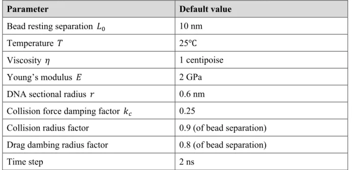
Figure 1.2: Simulated free-floating linear polymer chain
Illustration of simulated free-floating linear chain. Each red bead corresponds to a discretized chromosomal polymer unit. The connecting springs are shown as black line segments
connecting the beads. The example simulation contains 100 beads. (A) Initial geometry 𝑡 =
0 𝑠. 100 beads are located 10 nm away from the nearest neighbors at the resting length. (B)
𝑡 = 3𝑒_` 𝑠. (C) 𝑡 = 3𝑒_a 𝑠. (D) 𝑡 = 0.03 𝑠
A B
18
Brownian motion validation
The first step for validating the model is to test if the method of introducing thermal
force to represent Brownian motion for each bead is valid. In the simulation, a random force
is applied to each particle to simulate an identical dynamical displacement Brownian motion
leads to. This can be simply tested by generating multiple unconnected, free-floating particles
in the simulation. The collision force is turned off, making thermal force the only source of
external force for the dynamics. The mean squared displacement (MSD) from the simulations
are compared to the expected values of a particle experiencing Brownian motion (Rubinstein
& Colby, 2003):
〈𝑟/〉 = 𝑘=𝑇
𝜋𝜂𝑅𝑡 (1.20)
where 𝜂 is the viscosity of the fluid and 𝑇 is the temperature. R refers to the radius of the
bead. 𝑘= is the Boltzmann constant. Hence the MSD scales linearly with the elapsed time t.
This well-established result is used to confirm the validity of our thermal force term in
the model. Statistical tests have been applied to guarantee that the numerical design is
consistent with analytical results with probability above 95%.
Rouse time
One established analysis for Rouse models is the mode decomposition of the polymer.
In the Rouse model, the diffusion of a polymer chain in thermal dynamics is represented by
Brownian motion of beads connected by harmonic springs. Researches have shown that,
despite the initial geometry, the Rouse Chain will collapse into a random coil after a
particular amount of time from any initial configuration. Moreover, the time required to reach
the steady state can be calculated, given the environmental parameters, the polymer stiffness
and the size of the polymer (Rubinstein & Colby, 2003).The lowest order Rouse mode
19
𝜏: = 𝜂𝑏a
𝜋𝑘=𝑇𝑁/ (1.21)
Here 𝑁 is the number of segments and 𝑏 is the Kuhn length of the polymer. The parameters
corresponding to the environment are the following: 𝜂 is the viscosity of the fluid; 𝑇 is the
temperature. 𝑘= is the Boltzmann constant.
End-to-end distance
Another famous analysis for Rouse models is the end-to-end distance of the polymer,
which measures the length of the end-to-end vector of the polymer. After the polymer reaches
its equilibrium state and fluctuates as a random coil, the end-to-end distance obeys a certain
distribution. The mean of the end-to-end distance only depends on the stiffness and the size
of the polymer (Rubinstein & Colby, 2003). The mean end-to-end distance is
〈𝑅〉 = k𝑁𝑏/ (1.22)
for a Rouse model consisting of N particles, where b is the Kuhn length of the polymer (Kuhn
length = 2𝐿!).
Radius of gyration
One of the other commonly studied statistics in polymer analysis is the radius of
gyration which is defined as
𝑅"/ = 1
𝑁l‖𝒙𝒌− 𝒙𝒎𝒆𝒂𝒏‖/
c
HdF
, (1.23)
where N is the total number of particles on the chain. 𝒙𝒎𝒆𝒂𝒏 represents the mean position of
all the particles, and thus the right-hand side of the equation is the averaged squared distance
from all the particles to their mean position. Intuitively, the radius of gyration 𝑅" captures
20
This metric can be plotted over time as a proof of validation. There is close
relationship between 𝑅" and end-to-end distance. The expectation of the radius of gyration is
〈𝑅"〉 = k𝑁𝑏//6 (1.24)
for a Rouse model consisting of N particles.
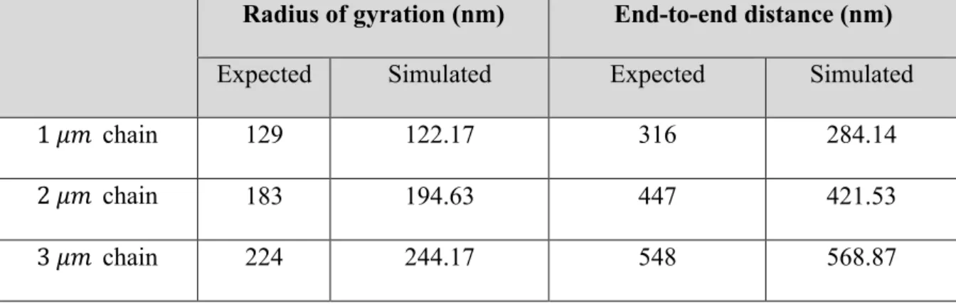
The simulated outputs are compared with analytical results by comparing radius of
gyration and end-to-end distance. Statistics from simulated results are averaged over samples
from 3 independent runs. The expected end-to-end distance and radius of gyration are
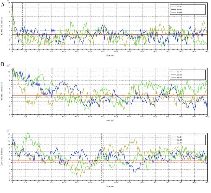
calculated from equations (1.22) and (1.23). See Figure 1.3, Figure 1.4 and Table 1.2 for
21
Figure 1.3: End-to-end distance plot of simulated free-floating linear chains
End-to-end distance plot for (A) 1 𝜇𝑚 linear chain, (B) 2 𝜇𝑚 linear chain, (C) 3 𝜇𝑚 linear chain. Red horizontal line refers to analytical end-to-end distance of the polymer governed by (1.22). Black dashed vertical line is the analytical Rouse time given by (1.21). All 3 runs for each experiment are independent, and the plot is constructed over 200 sampled instances for each run.
Seed1 Seed2 Seed3
0 0.01 0.02 0.03 0.04 0.05 0.06 0.07 0.08 0.09 0.10 0.11 0.12 0.13 0.14 0.15
10-7 0 1 2 3 4 5 6 7 8 9 10 Time (s) En d -t o -e n d d ist a n ce Seed1 Seed2 Seed3
0 0.01 0.02 0.03 0.04 0.05 0.06 0.07 0.08 0.09 0.10 0.11 0.12 0.13 0.14 0.15
10-7 0 1 2 3 4 5 6 7 8 9 10 Time (s) En d -t o -e n d d ist a n ce Seed1 Seed2 Seed3
0 0.01 0.02 0.03 0.04 0.05 0.06 0.07 0.08 0.09 0.10 0.11 0.12 0.13 0.14 0.15
22
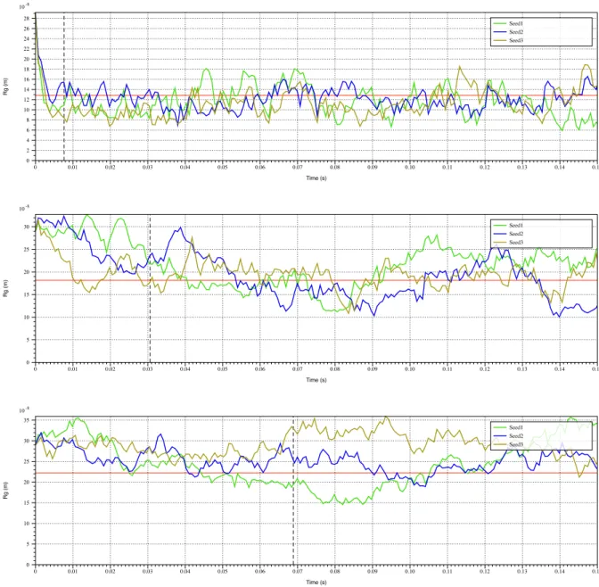
Figure 1.4: Radius of gyration plot of simulated free-floating linear chains
Radius of gyration plot for (A) 1 𝜇𝑚 linear chain, (B) 2 𝜇𝑚 linear chain, (C) 3 𝜇𝑚 linear chain. Red horizontal line refers to analytical 𝑅" of the polymer governed by (1.23). Black dashed vertical line is the analytical Rouse time given by (1.21). All 3 runs for each
experiment are independent, and the plot is constructed over 200 sampled instances for each run.
Seed1 Seed2 Seed3
0 0.01 0.02 0.03 0.04 0.05 0.06 0.07 0.08 0.09 0.10 0.11 0.12 0.13 0.14 0.15
10-8 0 2 4 6 8 10 12 14 16 18 20 22 24 26 28 Time (s) R g (m) Seed1 Seed2 Seed3
0 0.01 0.02 0.03 0.04 0.05 0.06 0.07 0.08 0.09 0.10 0.11 0.12 0.13 0.14 0.15
10-8 0 5 10 15 20 25 30 Time (s) R g (m) Seed1 Seed2 Seed3
0 0.01 0.02 0.03 0.04 0.05 0.06 0.07 0.08 0.09 0.10 0.11 0.12 0.13 0.14 0.15
23
Table 1.2: Averaged radius of gyration and end-to-end distance
Radius of gyration (nm) End-to-end distance (nm)
Expected Simulated Expected Simulated
1 𝜇𝑚 chain 129 122.17 316 284.14
2 𝜇𝑚 chain 183 194.63 447 421.53
24
The statistics shown in Table 1.2 are measured and calculated through samples from
simulation outputs to validate the simulation model. The simulations all start with linear
geometry. The equation governing the system is the same equation shown in (1.19), except
for that the collision force term is excluded from the equation, which is consistent with the
fact that the Rouse model does not take collision into consideration.
The good agreement with the Rouse time, expectation of end-to-end distance and
expectation of radius of gyration calculated in theory confirm accuracy of the numerical code
in the Rouse chain limit. Notice that even though the model is based on Rouse chains, there
are subtle differences in the force terms this reasonable deviation is acceptable.
Discussion
The polymer chain model is the basis for simulations for chromosomes. It stands out
in delivering fast real-time simulations of chromosome dynamics, provides alternative
approach to visualize the chromosomes in nucleus, and raise hypotheses that enlighten the
field of cell biology. To achieve this, additional modules need to be implemented and added
to the model in order to imitate real chromosomes. For instance, it is widely accepted that
SMC proteins play an important role in organizing chromosome structures, and thus it is
necessary to construct models for those proteins and embed them into the model. Moreover,
the chromosome obtains different geometrical structures and nuclear environment during
various stages of the cell cycle, meanwhile the default geometry simulates the chromosome
during the early stage of mitosis. Thus, programs simulating the dynamics of chromosomes in
other stages of the cell cycle could be achieved with modifications on the geometrical
constraints and environmental parameters.
Researchers have discovered profound knowledge on the fundamental structures of
25
imagination. There have been discussions on the choice of models for simulating
chromosomes. The choice of both the fundamental model and the influencing components
should be closely dependent on the scale of the particular model. For instance, to simulate the
dynamics of the entire genome in a budding yeast nucleus at a coarse scale, the worm-like
chain is utilized and the hinge force is neglected (Vasquez et al., 2016, Hult et al., 2017). For
this work, the simulation focuses on a finer scale of a single plasmid chromosome, down to
the finest scale of 10 nm. Therefore, polymer stiffness is relevant and a linear Hookean
approximation between beads is reasonable since beads do not get far enough apart to require
a nonlinear stiffening condition. There are possibilities for choices of separate fundamental
principles, for example a non-linear spring force law, to be discovered and to be tested under
26
CHAPTER 2: HISTONES AND CONDENSINS COMPACT CHROMOSOMAL STRUCTURES
Summary
The chromatin fiber wraps around an octet of histone proteins to form a nucleosome,
which is regarded as the basic structural element of DNA packaging. SMC proteins,
including condensin and cohesin, have been studied for their versatile function in compacting
and organizing the structure of chromosomes. They are indispensable components during the
process of chromosomal compaction. In this work, numerical models for condensin, one
major class of SMC proteins, and histones are carried out and embedded to the simulation
pipeline. They interact with DNA and create hierarchical loop structures along the chromatin.
The models for the proteins are constructed based on published experimental results, and
their functionalities are tested. The simulation results draw critical intuition into the
mechanism by which condensins and histones synergistically regulate the chromosome
structure, keeping the chromosome structure compact meanwhile dynamic.
Introduction
The geometrical structure of chromosome is of prodigious significance in cell biology.
The mechanisms that enables long chromosomes to be packaged into nucleus have attracted a
tremendous amount of attention. It has been discovered that the vast amount of DNA was
regulated in space not only by its double-helical spatial structure, but also maintained by
functioning proteins and polymer fluctuation in nuclear environment.
There are three major classes of proteins that manages the geometrical and topological
27
unlinking of intertwined DNA strands; the SMC proteins, which includes various classes of
proteins that take part in multiple aspects of DNA organization; Last but not least, the
DNA-binding proteins, which binds to DNA at their DNA-DNA-binding domains.
Among these proteins, we focus our interest on the particular types of proteins that
specifically contribute to DNA compaction. While DNA topoisomerases manage the
topological structures of the DNA supercoil in the winding point of view, this property is
parting from the scale and concentration of our simulation; In the family of SMC proteins,
there are two typical classes of proteins: cohesin and condensin, which have become popular
topics of research in cell biology in the past decade. While cohesins involve in sister
chromatid cohesion during DNA replication, we have focused on condensins, which implied
by their name are an essential factor in chromosome condensation; In various classes of
DNA-binding proteins, we fix our attention to histones, the protein that forms the basic
structural unit of chromatin in eukaryotes, because histones are also considered as one of the
key elements in chromosome packaging and compaction in the cell nucleus.
SMC proteins represent the family of complexes that participate in various forms of
chromosome organization. Among this large family of chromosomal ATPases, condensins
are large protein complexes that stand out specifically for chromosome condensation, and
have become a hot topic among researchers in the field. Not only their biochemical
composition, but also the dynamics they bring to the chromatin structure that have been
carefully studied. Each condensin complex is composed of five subunits, among them three
non-SMC regulatory subunits (one kleisin subunit, Brn1 and two HEAT-repeat subunits,
Ycs4 and Ycg1) and a pair of core SMC subunits, known as SMC2 and SMC4. Studies have
shown that condensins possess a wide variety of chromosome functions. For instance,
condensins contribute to the formation of chromosome territories (Bauer et al., 2012). The
28
shows that the condensin behaves as a mechanochemical motor that moves along DNA
(Terakawa et al., 2017), and there is biological evidence for loop extrusion hypothesis (Ganji
et al., 2018).
Although the existence and biochemical constitution of condensins have been
confirmed, how condensins help chromosome in condensation is still vague. Since a huge
amount of chromosome as well as an approximately equal concentration of proteins huddle
inside the nucleus, it is less possible for direct observation of interaction between condensins
and chromosomes in living cells. Alternatively, researchers separated DNA from nuclear
environment and successfully visualized the dynamics of DNA chain with condensin
activated in vitro. By applying a constant flow to the DNA for stretching, researchers clearly
observed a DNA loop structure formed by a condensin, and moreover the loop size grew
gradually at a varying rate. This behavior is called the loop extrusion of condensins. Although
this experiment showed condensins’ activity in full detail, the fact that the experiment was
not conducted in cell environment weakens the power of the experiment. The condensin
dynamics in the nucleus still remains uncertain.
Unlike condensins, histones form stationary subunits by acting as spools around
which DNA winds. This leads to shortened length (~7 times fold) of chromosomes. These
proteins are composed of 2 nearly symmetrical halves, essentially 4 histone proteins (Luger et
al., 1997). Each nucleosome is a highly stable unit. Besides chromosomal compaction
(Johansen & Johansen, 2006), histones also participate in chromatin regulation in diverse
processes, such as DNA repair (Supek & Lehner, 2017) and gene regulation. However, for
tethered chromosomes during early mitosis, both experiment and simulation suggest that
histones do not significantly decrease the signal size of the marked region of dicentric
plasmid chromosomes. How histones compact chromosomes in particular geometrical
29
Condensins and histones are claimed to be proteins that contributes to chromosome
packaging and condensation. Yet the detailed demonstration that explains the underlying
mechanistic basis remains veiled. Here we take another approach to learn how condensins
and histones transform the properties of the chromosome polymer and condenses the strand.
We construct models for histones and condensins intuited by experimental results and involve
them in the polymer chain model. Tests and comparisons with statistics from experiments
need to be conducted to validate the model. Then we will take a glimpse at the structural
changes the proteins deliver to the system, and clearly observe the mechanism of how
histones and condensins compact and condense the chromosome structure.
Methods
Histones
Experimental observations have provided clear observation report in vivo on the
structure of histones at a high resolution (Luger et al., 1997). On average 147 bp of DNA
wraps 1.65 times around the histone octamer at a very high occurrence along the chain.
Essentially histones attach to the chromatin spine every 200 bp across all eukaryotic
genomes. Then these histones build higher order structures by forming assemblies among
nucleosomes and stabilized by linker histones. Study have also shown that histones obtain
intrinsic periodical turnover. Extensive histone exchange happens in nucleus, independent of
cell replication. Furthermore, histone protein H3 behaves as a tension sensor that helps
regulating the cell during mitosis (Luo et al., 2016). DNA unwind from the histone protein
spool under high tension during the dividing process. These are both mechanisms for histones
to self-regulate. Moreover, histone synthesis is reported to be dynamically regulated by the
modulation of the half-life of histone mRNA (Morris et al., 1991), which implies that histone
30
Histones in our simulation are modeled according to published results (Luger et al.,
1997). In the simulation, histones are modeled as multiple stationary 7-bead subloops along
the chain (each unit represents ~30 𝑏𝑝 × 7 = ~210 𝑏𝑝 size of nucleosome). Those
subloops are formed by applying virtual springs at the attachment sites. The polymer is fully
loaded by histones by default in simulation due to high enrichment of nucleosomes in
observations. Each histone unit periodically attaches to and detaches from the chromatin
chain to simulate the turnover of histones observed in vivo. The turnover mechanism is
achieved by setting an intrinsic timer to each unit. One histone unit switches status once the
timer exceeds the predefined deadline. In simulation, in order to stochastically vary the
average number of active histones, one can tune either the total number of histones in the
simulation or the on/off period of the histones. Moreover, winding DNA under high tension is
capable of unwinding histones, which is consistent with observations of force-dependent
unwinding and rewinding mechanism.
In the simulation neither the mass of histones nor the higher order structural
interactions between nucleosomes are considered upon this point. We focus instead on the
consequences of the loop structures. Figure 2.1 A shows an example of the geometry of the
chromosome while interacting with a histone. The ring-like substructure remains static until
the histone detaches from the DNA.
Condensins
The biochemical composition of condensins have been well studied (Hirano et al.,
1997). They are known as the key component in cell organization and compaction. During
metaphase, the spindle axis is enriched with condensins (Stephens et al., 2011). A natural
assumption on the behavior of condensins is that condensins help to organize the DNA
31
distributed into the daughter cells during mitosis. However, the underlying mechanistic
function condensins perform when interacting with the chromatin remains unknown, with a
number of hypothesis and corresponding models illustrating different possible explanations
(Sakai et al., 2018; Thadani et al., 2012).
In a previous study, condensins were modeled as static springs (J Lawrimore et al.,
2016). These protein complexes are able to form large subloops along the chromatin chain.
Later, with Terekawa et al. published their examination of the behavior of single condensing
complexes on DNA sheets, condensins are confirmed to obtain mobility while they are
actively creating loops (Terakawa et al., 2017). In their work, condensins are regarded as
biological motors that translocate along the DNA at a rate of about 60 bp/s.
A recent work by Ganji et al showed the motion pattern of condensins, which they
name it the loop extrusion (Ganji et al., 2018). By utilizing real-time imaging techniques,
they are able to visualize the behavior of a single condensin while binding to a separated,
flow-stretched DNA in vitro. Provided energy, the condensin complex is capable of creating
a loop on that DNA and continuously expanding that loop. Additionally, they found that the
extrusion behavior does not possess a constant rate. The extrusion slows down as the DNA is
further stretched, which is explained as another influential hypothesis: the loop extrusion rate
of condensins depends on the tension along the binding DNA. This publication has been
revolutionary in the field, leading to numerous downstream studies.
We developed a prototype condensin model that is able to translocate along the DNA
chain while extruding loops. Intuitively, each condensin complex in the model can be
considered as a person grabbing a rope. As the person is grabbing the rope towards him, an
expanding loop will form. When the person experiences an extreme tension along the rope, a
sudden release is triggered. To be more precise, the condensins are modeled as a dynamic
32
heterogeneous. One end is more dynamic in the sense that it constantly reaches out to distant
segments along the chain. We call this end “the weak end”. Once the weak end lands on the
chromosome, the core spring pulls the attachment site towards the other end, which is called
“the strong end”, and thus a loop is formed. The strong end is relatively stable. It generally
remains stationary, only releases the chain once the condensin core spring attains too much
tension. After detachment, the condensin shrinks to its initial configuration and attach to the
chain at a segment closer to the weak end. This mechanism allows the condensin complexes
to form a loop and translocate simultaneously. This model is similar to established condensin
model (Josh Lawrimore et al., 2017). However, the performance of this model is not optimal.
It fails to reconstruct the extremely compact chromosome structure.
An up-to-date model of condensin complexes we construct is based on the loop
extrusion observation published by Ganji et al. The main difference from our previous model
can be interpreted also by the “rope pulling” analogy. In this model, the person does not
release the rope upon excessive tension. The hypothetical model of such a complex is a ring
structure that anchors on a segment of DNA. The rest portion of DNA is grabbed and pulled
by the complex through its ring structure and completes the extrusion activity. In our model,
each complex is modeled as a spring attaching to the DNA strand, with one end anchored at a
fixed site, which is called ‘the strong site’. The strong end does not release upon high local
tension, comparing to our previous model. The other attachment site of the complex, ‘the
weak site’, moves along the chain, attach to a farther segment of the DNA, and then the
spring pulls the two ends close again to complete the extrusion activity. A customized
function governs the rate at which the weak site takes one action in order to simulate the
decaying extrusion rate shown in experiments. Moreover, after a predefined period of
extrusion, the spring releases and restart to extrude another loop. Instead of a multi-step
33
accordance with the sudden disruption of the condensin loop in experiments. Figure 2.1(B) -
(D) illustrate how a condensin loop evolves in a short period. The extrusion rate was
amplified compared with real simulations, for a clear observation of the loop extrusion
behavior.
The histones and condensins we introduce into the simulation do not conflict with
each other. Each bead can be winding around histones while being a portion of the condensin
extruded loop at the same time. The proteins are able to attach to every bead, except the two
end beads of the circular chromosome which are used to model sister centromeres. The
program will parse the coordinates for all beads and save them into the output file, same as
the output from the model in Chapter 1. However, one can choose to output the positions of
the attachment sites of the proteins at every saving stride for further studies. By default, the
indices of condensins’ attachment sites are also written into output file. A list of tunable
34
Figure 2.1: Illustration of histone model and condensin model
(A) In simulation, a histone creates a small, static loop at its attachment site. (B) Initialization of condensin model. The blue beads represent the substructure formed by a single condensin complex. (C) The condensin starts to extrude a loop. (D) The condensin forms a large, dynamic loop.
A B
35
Table 2.1: Tunable parameters corresponding to DNA-binding proteins
Parameter Default value Parameter corresponding class
Number of histones 50 Histone
Histone loop size 7 Histone
Mean On 5 𝑚𝑠 Histone
Mean Off 0 𝑠 Histone
SD 0.1 𝑚𝑠 Histone
Detach Off Histone
Detach threshold 30 𝑛𝑚 Hisone
Number of condensins 6 Condensin
Dynamic extrusion On Condensin
Judge time 20 𝜇𝑠 Condensin
Increment 10 𝑛𝑚 Condensin
Extrusion decay rate 1 Condensin
Detach 1 Condensin
Mean On 11.3 𝜇𝑠 Condensin
SD On 4.3 𝜇𝑠 Condensin
36
Data analysis methods
In the Bloom Lab at Department of Biology, University of North Carolina at Chapel
Hill, timelapses of a fluorescent-tagging synthesized dicentric plasmid chromosome was
obtained and used for analyses. The chromosome is isolated and circular with two
centromeres when it loses the ability to replicate (autonomously replicating sequence, ARS)
and becomes an ideal target for chromosomal analyses. It is labeled with a 5.5 kbp
tetO/TetR-GFP array (Dewar et al., 2004) for observation purpose (Figure 2.2 A). The chromosome is
circular, with two centromeres located asymmetrically, creating a longer arm and a shorter
arm. These two portions of the chromosome are called “the loose arm” and “the tight arm”,
respectively. The GFP portion is located in the middle of the loose arm.
Original biological data are a series of signal images from the fluorescent portion of
the dicentric plasmid chromosome. The image series are obtained from parsed time lapses
every 30 seconds for 20 minutes in vivo. Due to the restriction of resolution, the images are
blurry bright spots. Characteristics of the chromosome can be represented by certain statistics
from the images. Typical statistics include measuring the “signal length”, which is generated
by a custom MATLAB GUI (J Lawrimore et al., 2016). In short, the signal length is the
major axis length of the minimum oval covering the signal. In some cases, the “signal width”,
the minor axis length of the oval, is also taken into consideration.
Moreover, we observe frequent oscillation in the size of the signal in vivo. To
examine the signal variations, we create the density map to show change in signal length as a
function of temporary signal length. The change in signal length is measured by the
difference between the current signal length and the signal length observed one following
timestep. The frequency is displayed by color code where red is the most dense and blue is
37
In order to directly compare simulation data with biological observations, we
convolve the corresponding GFP-tagging fluorescent portion of simulation result with a
point-spread function using the program called Microscope Simulator 2 (Quammen et al.,
2008). This method allows to convert simulation results which are exact positions to vague
signals with great consistency. Then the simulated images are analyzed using a custom
MATLAB program that automatically converts the simulated images into binary masks and
uses the REGIONPROPS function in MATLAB to measure the signal lengths. The resulting
statistics can be directly compared to the experimental results.
Results
Experimental Results
The signal length histogram (Figure 2.2) reveals a right-skewed distribution, with
mean and median between 600-700 nm. The most frequently observed signal length is
between 500-600 nm, showing a very compact structure of the signal. The density heatmap in
addition shows frequent signal fluctuation by several observations located off the center of
the y-axis. The fit for the distribution supportively suggests the skewness of the distribution
(Figure 2.2 C). Instead of a symmetric Gaussian distribution, a bimodal 2-term Gaussian
distribution fits the data better.
The plasmid signals reveal the characteristics of the dynamics of plasmid
chromosomes: condensed while dynamic. The compactness is essential in chromosomal
organization through cell cycles. Meanwhile, the mobility of chromosome is indispensable.
Studies have shown the close correspondence between chromatin motion to nuclear fields,
38
Figure 2.2: Dicentric plasmid chromosome signal and signal length analyses
(A) The signal of WT plasmid chromosome with tetO/TetR-GFP array. (B) Density heat map of change in signal length plotted against signal length. (C) Histogram of plasmid
chromosome signal length in normalized frequency. The histogram is also fitted with one-term and two one-term Gaussian distributions. The fit is evaluated through 𝑅/ statistics. Greater
statistics implies better fit. A
C
39
Simulation Results: histones and condensins compact the dicentric plasmid
To investigate the functions of the structural proteins of interest, we compare the
simulation outputs by gradually add components to the system and observe the intermediate
results. That is, we compare the signal length from 4 distinct systems: the raw polymer chain
system introduced in Chapter 1; the polymer chain system with histones; the polymer chain
system with condensins; and finally, the polymer chain system with both histones and
condensins. We extract the simulated signal length by similar approach as in experiments,
transform the signals to acquire the metrics and directly compare to the statistics from
experimental results. Reasonable errors are tolerable between simulated results and
experimental results. The ultimate goal is to observe similar properties revealed by
experiments: condensed signals with intensive variation.
The raw polymer chain model shows large signal lengths, with rare fluctuation
(Figure 2.4 A, B). The simulated signal lengths are symmetrically distributed and are most
frequently observed to be between 800 and 900 nm, combining up to ±150 nm of variation.
While the thermal fluctuation is acting as the only external source for energy, the system
lacks the ability to oscillate at a comparable scale to real chromosomes. Moreover, the large
averaged signal length suggests that additional components is influencing the system and
compacting the structure.
When histones are introduced, we observe a stable structure with very little
fluctuation (Figure 2.4 C, D). The compact geometry created by histones tighten the chain,
which lead to less overall fluctuation in space (Figure 2.3 B). In other words, histones stiffen
the polymer chain by creating substructures. However, histones alone fail to reduce the signal
size. Observations with 800-900 ± 50 nm signal lengths occupy over 90% of the total
observations. Compact signals, such as the small round signals observed in vivo, never
40
geometrical structure of the plasmid leads to this consequence. One can imagine the effective
compacting effect of histones for free-floating chromosomes in other cell cycles than mitosis.
However, there must be supplementary mechanisms that lead to the condensed structure of
dicentric plasmid chromosomes.
When condensins are included in the model, the signals show very different
dynamics. The vital distinction is the intense fluctuation. One can observe the signal
oscillation through both the geometry and the plots (Figure 2.3 C, Figure 2.4 E, F). In the
evolution movie of the polymer, condensins keep extruding loops, creating traversing large
scale substructures. These active motors bring energy to this system, causing more
observations with extreme structures. Through the histogram, a great amount of data spread
out to either small signal length down to 400 nm or large signal length up to 1200 nm. This
signal variation confirms with experimental data. However, the averaged signal length is not
shifted. Most of the signals are still 800-900 nm in length, and the distribution shows no
right-tailed skewness.
The best approximation to experimental results comes from simulations combining
both histones and condensins. Both key factors, the condensed structure and the intense
fluctuation, are satisfied. The most frequent signal lengths are around 500 nm, and the
distribution is right-skewed (Figure 2.4 G). The heatmap shifts its center from 800 nm to 500
nm while maintaining the vertical spread (Figure 2.4 H). Also, it maintains the ability to
create extreme observations up to 1200 nm. The box plot shows direct comparison of
averaged signal lengths (Figure 2.4 I). The synergetic mechanism of histones and condensins
successfully reduce the signal length while maintaining mobility. Presumably, the mobility is
guaranteed by condensins, since introducing condensins alone will greatly amplify the