Multi-objective Optimal Location of Optimal Unified Power Flow Controller (OUPFC) through a Fuzzy Interactive Method

(1)

Sharif University of Technology

Scientia Iranica

Transactions D: Computer Science & Engineering and Electrical Engineering www.scientiairanica.com

Multi-objective optimal location of Optimal Unied

Power Flow Controller (OUPFC) through a fuzzy

interactive method

A. Lashkar Ara

a;

_{, M. Shabani}

a

_{and S.A. Nabavi Niaki}

b

a. Department of Electrical Engineering, Dezful Branch, Islamic Azad University, Dezful, P.O. Box 313, Iran. b. Department of Electrical and Computer Engineering, University of Toronto, Toronto, ON M5 S 3G4, Canada. Received 24 June 2014; received in revised form 28 March 2015; accepted 16 June 2015

KEYWORDS OUPFC; UPFC; FACTS;

Optimal location; Multi-objective; Fuzzy interactive method.

Abstract.This paper presents a fuzzy interactive approach to nd the optimal location of Optimal Unied Power Flow Controller (OUPFC) device as a multi-objective optimization problem. The problem formulation is based on Optimal Power Flow (OPF) problem while the metric function and weighting method are added to ensure the collaboration among objective functions. The objective functions are the total fuel cost, power losses, and system loadability with and without the minimum cost of OUPFC installation. The proposed algorithm is implemented on IEEE 14- and 118-bus systems. The solution procedure uses nonlinear programming with discontinuous derivatives (DNLP) to solve the optimal location and settings of OUPFC device to enable power system dispatcher to improve the power system operation. The optimization problem is modeled in General Algebraic Modelling System (GAMS) software using CONOPT solver. Furthermore, the results obtained by OUPFC are compared with those of the Unied Power Flow Controller (UPFC) device. The OUPFC is outperformed by UPFC in the power system operation from the economic and technical point of view.

1. Introduction

The optimum operation of an interconnected power system involves dispatcher concerns such as optimal choice and allocation of Flexible AC Transmission Systems (FACTS) devices as power ow controllers. Optimal Unied Power Flow Controller (OUPFC) is a member of FACTS controllers that can provide the necessary functional exibility for optimal power ow control through phase angle control. It is composed of a conventional Phase Shifting Transformer (PST) and a scale-down Unied Power Flow Controller (UPFC).

*. Corresponding author. Tel.: +98-641-6260051; Fax: +98-641-6260890

E-mail addresses: [email protected] (A. Lashkar Ara); [email protected] (S.A. Nabavi Niaki)

The steady-state model of OUPFC and its operational characteristics are introduced in [1].

The multi-objective OPF problem considering FACTS devices is addressed in many technical liter-ature. In [2], the best location of PSTs has been determined by genetic algorithm to reduce the ows in heavily loaded lines resulting in increased system loadability and reduced generation costs. The best op-timal location of FACTS devices, in order to reduce the generation costs along with the device's cost using real power ow performance index, has been reported [3]. A hybrid tabu search and simulated annealing has been proposed to minimize the generator fuel cost in OPF control with multi-type FACTS devices [4]. The opti-mal location of FACTS devices has been found using the Particle Swarm Optimization (PSO) technique for considering system loadability and installation cost [5].

(2)

In [6], the multi-objective optimal location of PST, UPFC, and OUPFC has been considered using the "-constraint method. The contingency-based optimal location of UPFC and OUPFC has been investigated under a single-line contingency [7].

Several dierent methods have been widely ap-plied for solving various power system problems such as optimal location and OPF problems. These methods can be divided into two main categories:

(i) Mathematical methods that include nonlinear programming [8], quadratic programming [9,10], linear programming [11,12], Newton-based tech-niques [13,14], sequential unconstrained minimiza-tion [15], interior point [16,17], and minimum cut algorithm [18],

(ii) Intelligent methods that include Evolutionary Programming (EP) [19], Genetic Algorithm (GA) [20-22], Dierential Evolution (DE) [23], Articial Neural Network (ANN) [24], Simulated Annealing (SA) [25,26], Articial Bee Colony rithm (ABC) [27], PSO [28], harmony search algo-rithm [29], and gravitational search algoalgo-rithm [30]. Although some of the mathematical methods have excellent convergence characteristics, some drawbacks of these methods are [31]:

- The solution converges to a local optimum instead of a global optimum, depending on the selected initial values;

- Each technique is suitable for a specic kind of optimization problem based on the mathematical nature of the objectives and/or constraints;

- Some theoretical assumptions, such as convexity, dierentiability, and continuity, are built into these methods which may not be suitable for the OPF problem;

- They are not able to interact with the decision-maker through optimization process.

In addition, the intelligent methods have been success-fully used to solve the optimization problems in which global solutions are more preferred than local ones, or when the problem has non-dierentiable regions. But these methods have some drawbacks, too, such as: - These methods require signicantly large

compu-tations and are not ecient enough for real-time systems that need to quickly change the system; - Implementation of these methods is dicult; - They generate a Pareto solution set; the

decision-maker must select the best compromise solution through Pareto solutions by a decision-making ap-proach;

- They are stochastic and cannot strictly gure on solutions optimally;

- They are not able to interact with the decision-maker through optimization process.

In order to handle the mentioned problems, the fuzzy optimization approach is used to solve the multi-objective optimization problems. The objective functions and constraints are considered as modied constraints in terms of their fuzzy membership functions. The model is constructed by denition of sets of membership functions for each constraint and objective function. Therefore, the main purpose of a fuzzy optimization problem is to maximize all membership functions at the same time. This is usually done using a formulation similar to the min{max formulation for the multi-objective optimization [32]. Consequently, fuzzy optimization lends itself to multi-objective optimization where additional multi-objective functions are modeled as constraints. Moreover, the conicting degree among objectives and the designer's preferences are nearly neglected in many fuzzy multi-objective optimization models; however, they are still an ongoing research topic.

In this paper, an interactive fuzzy multi-objective optimization method, incorporated in the metric func-tion and weighting method, is proposed to enable the operator to interact with the algorithm through opti-mization process in contrast to other multi-objective methods.

To the best of our knowledge, no research work has been developed to locate and allocate the OUPFC device through the fuzzy interactive multi-objective optimization. The main contribution of this paper is to nd the optimal location of OUPFC based on OPF problem incorporated in the metric function and weighting method as the multi-objective optimization problem. The objective functions are classied into four categories:

(i) The total fuel cost; (ii) Active power losses; (iii) System loadability;

(iv) Installation cost of the FACTS device.

The optimal location and settings of OUPFC are determined on the IEEE 14-, and 118-bus test sys-tems to optimize these objective functions simulta-neously. The optimization problem is modeled as a nonlinear programming with discontinuous deriva-tives (DNLP) problem in General Algebraic Modeling System (GAMS) software and solved using CONOPT solver [33]. Furthermore, in order to highlight the per-formance and applicability of the OUPFC, its results are compared with those of UPFC.

(3)

mod-eling of FACTS controllers are studied in details in Section 2. Section 3 contains the problem formulation of OPF incorporated in the FACTS device, including variables, objective functions, and constraints. The multi-objective optimization problem is presented in Section 4. The simulation results and the optimal settings and the best location of OUPFC and UPFC are reported in Section 5.

2. Modeling of FACTS devices 2.1. Modeling of OUPFC [1]

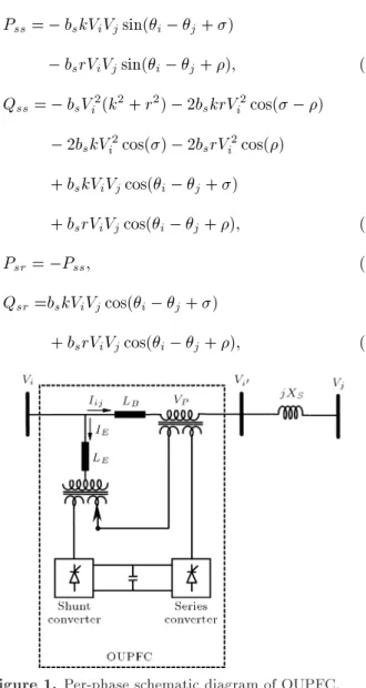
The OUPFC is comprised of a PST and a UPFC, as shown in Figure 1. The power injection model of the OUPFC is shown in Figure 2 where:

Pss= bskViVjsin(i j+ )

bsrViVjsin(i j+ ); (1)

Qss = bsVi2(k2+ r2) 2bskrVi2cos( )

2bskVi2cos() 2bsrVi2cos()

+ bskViVjcos(i j+ )

+ bsrViVjcos(i j+ ); (2)

Psr = Pss; (3)

Qsr =bskViVjcos(i j+ )

Figure 1. Per-phase schematic diagram of OUPFC.

Figure 2. The power injection model of FACTS devices.

Figure 3. Basic schematic diagram of UPFC.

where k is the transfer ratio of PST; is the PST phase angle; r is the radius of the UPFC operating region; is the UPFC phase angle; bsis 1=(XS+ XB) where XS

is the transmission line reactance; and XB is the series

transformer leakage reactance. 2.2. Modeling of UPFC

The basic schematic of the UPFC is shown in Figure 3. The power injection model of the UPFC is same as the OUPFC of Figure 2 where:

Pss= bsrViVjsin(i j+ ); (5)

Qss= bsrVi2(r + 2 cos())

Psr = Pss; (7)

Qsr= +bsrViVjcos(i j+ ); (8)

where r is radius of the UPFC operating region; and is the UPFC phase angle [34].

3. Problem formulation

The problem formulation is based on a multi-objective OPF problem to make trade-o between objective func-tions and optimize four objective funcfunc-tions simultane-ously while satisfying several equality and inequality constraints. The objective functions and constraints are explained in the following.

3.1. Objective functions

The objective functions are dependent on the system requirements and on the system operator concerns. Therefore, the objective functions of this paper are the total fuel cost, active power losses, system loadability, and installation cost of the FACTS device.

(4)

3.1.1. Total fuel cost

The quadratic fuel cost functions are used to minimize the total operating cost as the objective function. The objective function of the total fuel cost can be formulated as follows [35]:

F1(Pi) = NG

X

i=1

Ci(PGi) = NG

X

i=1

0i+ 1iPGi

+ 2iPGi2 ($/h); (9)

where PGi is generator active power output at bus i;

0i, 1i, and 2iare cost coecients of unit i; and NG

is number of generators. 3.1.2. Active power losses

Loss minimization is very important in the power system operation and tends to reduce the reactive power ow in the power system. It can be expressed as follows [36]:

F2(V; ) = n

X

i=1 n

X

j=1

ViVjYijcos(ij+ j i); (10)

where Vi and i are voltage magnitude and angle of

bus i; Yij and ij are the elements of admittance

matrix magnitude and angle in row i and column j, respectively; and n is number of buses.

3.1.3. System loadability

The power system operator usually prefers some fur-ther loading margins to decrease the risk of load variations, particularly in weak connections of the net-work. Therefore, the objective function of the system loadability can approximately remedy the maximum loading limits of the transmission lines and the dynamic power oscillations of the system that can be described as [37,38]:

F3= (x; u); (11)

and can be obtained by assuming constant power factor at each load in both real and reactive power balance equations as follows:

PG PD= fp(x; u); (12)

QG QD= fq(x; u); (13)

where PG and QG are the vectors of generators real

and reactive power, respectively; PD and QD are the

vectors of loads real and reactive power, respectively; fp and fq are the vectors of real and reactive power

ow equations, respectively; and x and u are sets of dependent and control variables, respectively.

3.1.4. FACTS investment cost

Since the installation of FACTS device is an invest-ment issue, it interests the operator to decrease the

total operating cost including its cost while the other objectives are considered. Therefore, the cost of FACTS installation is minimized in the multi-objective optimization framework. It can be mathematically formulated as follows:

F4= _{8760 5}CFACTS ($/h); (14)

where CFACTSis the cost of FACTS installation in US$.

The OUPFC and UPFC cost functions are taken [6,39] as follows:

COUPFC=[(12 SPST) + ((0:0003SUPFC2

0:2691SUPFC+ 188:22) SUPFC)]

1000; (15)

CUPFC=(0:0003SUPFC2 0:2691SUPFC+ 188:22)

SUPFC 1000; (16)

where SFACTSis the operating range of FACTS devices

in MVA. In this paper, a ve-year period is assumed to usefully apply FACTS devices.

3.2. Constraints

The constraints of OPF problem can be divided into two categories: equality and inequality constraints. 3.2.1. Equality constraints

The equality constraints include active and reactive power balance equations for each bus as follows [35]:

PGi+PFACTSi=PDi+ n

X

j=1

ViVjYijcos(ij+j i)

8i 2 1; 2; ; n; (17)

QGi+QFACTSi=QDi+ n

X

j=1

ViVjYijsin(ij+j i)

8i 2 1; 2; ; n; (18) where PGi and QGiare the generator active and

reac-tive power at bus-i, respecreac-tively; PDi and QDi are the

load active and reactive power at bus-i, respectively; PFACTSi and QFACTSi are the injected active and

reactive powers by the FACTS device, respectively. 3.2.2. Inequality constraints

Inequality constraints represent the following limits on the active and reactive output power of generators, bus voltages, transmission lines loadings, and FACTS operational parameters [31].

a. The generators active and reactive output power is restricted by its lower and upper limits as follows:

(5)

Pmin

Gi PGi PGimax 8i 2 NG; (19)

Qmin

Gi QGi QmaxGi 8i 2 NG: (20)

b. Voltage magnitude of the buses is limited in the region dened by the operator in the following form:

Vmin

i jVij jVimaxj 8i 2 n: (21)

c. The apparent power ow of transmission line l is lower than its maximum value, i.e.:

jSlj jSmaxl j 8l 2 1; 2; ; NL: (22)

d. The FACTS parameters are bounded as fol-lows [1,34]:

rmin_{r r}max

minmax

9 > > > > = > > > > ;

for OUPFC; (23)

rmin_{r r}max

minmax

9 =

; for UPFC: (24) 4. Interactive fuzzy multi-objective

optimization algorithm

Generally, the multi-objective optimization problem at-tempts to nd feasible solutions to optimize a vector of objective functions F (x) = fF1(x); F2(x); ; Fn(x)g

while the constraints are satised. The problem can be formulated as follows:

minimize or maximize:

F (x) = fF1(x); F2(x); ; Fn(x)g;

subject to:

hi(x) = 0; i = 1; 2; ; I;

gj(x) 0; j = 1; 2; ; J;

Xu

k Xk Xkl k = 1; 2; ; k; (25)

where F (x) is a vector of objective functions which can be minimized or maximized simultaneously; hi(x)

and gj(x) are equality and inequality constraints,

respectively; Xu

k and XKl are upper and lower bounds

of variables, respectively. It is noted that the problem should be modeled as the fuzzy optimization frame-work. Therefore, the process of fuzzy implementation is explained in the following.

Table 1. Computed payo table by single objective optimization for each function.

F1 F2 F3 F4

(min F1; F2; F3; F4) F1(x1) F2(x1) F3(x1) F4(x1)

(F1; min F2; F3; F4) F1(x2) F2(x2) F3(x2) F4(x2)

(F1; F2; max F3; F4) F1(x3) F2(x3) F3(x3) F4(x3)

(F1; F2; F3; min F4) F1(x4) F2(x4) F3(x4) F4(x4)

4.1. Single objective optimization

The search space of multi-objective optimization is usually well dened by single objective optimization. Therefore, each objective function is optimized while the corresponding values of other objective functions are calculated at the optimal point. Consequently, the payo table is constructed as shown in Table 1.

In order to normalize each objective function, its maximum and minimum values are directly obtained from the payo table as follows:

mi= Fi(xi) i = 1; 2; 3; 4;

Mi= max_j=1;2;3;4fFi(Xj)g i = 1; 2; 4;

Mi= min_j=1;2;4fFi(Xj)g i = 3; (26)

where x

i is the optimal solution of ith objective

function as the Pareto optimal solution; mi and Mi

are the best and worst values of ith objective function, respectively.

4.2. Developing the interactive constraint One of the most important features of a fuzzy multi-objective optimization is presentation of candidate solutions in an interactive process. The general idea of interactive methods is to determine a good compromise solution integrating preferences of the operator. The operator's preferences can be consistently represented in the optimization model using the interactive process, although the objective functions naturally conict with each other. In this paper, the interactive process is implemented by the metric function as dened by the following equation [40]:

d(x) =

v u u tXn

i=1

Mi Fi(X)

Mi mi

; (27)

where belongs to the interval [1; +1) and usually equals to 2; X is the vector of single objective solutions; the metric function is minimized to evaluate the opti-mum X using the common min-max method as follows:

F (X) = min

x maxi

Mi Fi(X)

Mi mi

: (28)

(6)

de-ned by the operator can be incorporated in the metric function as additional constraints in the optimization problem:

wiM_Mi Fi(X) i mi

"; (29)

related to minimizing the ith objective function, wjFj_m(X) Mj

j Mj

"; (30)

and to maximizing the jth objective function, and

n

X

i=1

wi= 1; (31)

where wi is the importance degree of the ith objective

function and " is the allowable degree of deviation from the optimal solution obtained by the single objective optimization.

The ideal value of the deviation degree is equal to 0. Therefore, the additional constraints, as equality constraints in the optimization problem, are equal to each other, i.e.:

wi i=1;2;4

Mi Fi(x)

Mi mi

= wj

j=3

Fj(x) Mj

mj Mj

; (32) and:

4

X

i=1

wi= 1:

The collaboration among objective functions and the importance degree of each objective function are con-sidered by adding these equality constraints into the multi-objective optimization problem. Furthermore, the relative deviations of each objective function from its optimal value can be minimized.

4.3. Constituting membership functions

The main idea is to simultaneously optimize objec-tive functions and constraints in the fuzzy optimiza-tion [41]. To implement this idea, the multi-objective optimization problem can be converted into a single-objective optimization by the fuzzy optimization strat-egy. Therefore, the objective functions and constraints are reformulated by using fuzzy membership functions to reect the satisfaction degree of a given solution. The rst step is a fuzzication process of the objective functions and the constraints. This procedure converts the objective functions Fi(x) and constraints gj(x) into

pseudogoals Fi(x) and gj(x), respectively.

The membership functions for F1, F2, and F4are

provided by linear monotonically decreasing function when these objectives are in between their maximum

and minimum values obtained by Eq. (26). In other words, the degree of satisfaction decreases while these objectives increase from mi to Mi (i = 1; 2; 4). The

mathematical formulation is expressed as follows [40]: _F~_i=

8 > < > :

1 Fi(x) mi Mi Fi(x)

Mi mi mi<Fi(x)<Mi;

0 Fi(x) Mi

i=1; 2; 4: (33) Similarly, the membership function of F3is determined

by an increasing function when it is in the range between M3and m3. These membership functions can

be written as: F~i=

8 > < > :

0 Fi(x) Mi Fi(x) Mi

mi Mi Mi< Fi(x) < mi;

1 Fi(x) mi

i = 3: (34) In the conventional OPF, from other viewpoints, the equality and inequality constraints can be catego-rized into hard and soft constraints [42]. The hard constraints comprise the active and reactive power balance equations, output power of generators, bus voltages, and FACTS operational parameters. Because of technical and physical limitations, violations of these limits are not justiable in any power system. On the other hand, the limits for the transmission line ows are soft constraints. The word \soft" signies that the constraint is not absolutely enforced. Small violations of these limits sometimes can be acceptable, for example, when occurring especial conditions such as line over loaded or contingency. Normal and emergency limits are two usual limits for each constraint of the transmission line ows. The operators desire to operate the system in optimum performance within normal limits while small violations of the normal limits are allowed. However, the emergency limits can never be violated and are considered as hard limits. These practical considerations of constraint limits are not satisfactorily formulated in a conventional OPF.

Soft constraints on membership functions are made based on the desired lowest limit (bj) and the

highest limit (bj+ dj) as normal and emergency limits

of the transmissions line ows. The membership functions of inequality constraints are characterized by trapezoidal functions as follows [40]:

~gj =

8 > < > :

1 gj(x) bj [(bj+dj) gj(x)]

dj bj gj(x) bj+ dj

0 gj(x) bj+ dj

(35) 4.4. Fuzzy multi-objective optimization

modeling

After the fuzzication process, membership of the optimal function can be found by the aggregation of

(7)

all the pseudo-goals and constraints. In the com-putation of fuzzy maximum function, the degree of satisfaction for fuzzy functions and fuzzy constraints can be represented by a membership variable . The membership variable is dened as the minimum of all the membership functions of the fuzzy functions and fuzzy constraints. This procedure can be formulated through the following equations [41]:

=D(x) = minfF1(x); ; F4(x); g1(x);

; gn(x)g: (36)

Using operator maximum, the optimal solution is computed as:

max

2[0;1] = max2[0;1]minfF1(x); ; F4(x); g1(x);

; gn(x)g: (37)

Finally, the interactive fuzzy multi-objective optimiza-tion is modeled as follows [40]:

maximize: ; subject to:

F~i(x) i = 1; 2; 3; 4;

~gi(x) i = 1; 2; ; n;

wi i=1;2;4

Mi Fi(x)

Mi mi

= wj

j=3

Fj(x) Mj

mj Mj

;

4

X

i=1

wi = 1;

0 1; Xu

k Xk Xkl: (38)

5. Case studies

The proposed method is applied to the IEEE 14-, and 118-bus test systems to verify its eectiveness to optimally locate OUPFC and UPFC devices. It is implemented in GAMS and modeled as a DNLP problem. The optimization problem is solved using CONOPT solver [33]. Data on the IEEE test systems are taken from [43]. Parameters and limits of the OUPFC and UPFC devices are given in Appendix A.

The CONOPT is used to solve static and dynamic large-scale nonlinearly constrained optimization prob-lems. The GAMS/CONOPT solver is the link between the GAMS and CONOPT to solve the problem. It has a fast method for nding a rst feasible solution that is

particularly well suited for models with few degrees of freedom. It can also be used to solve square systems of equations without an objective function corresponding to the constrained nonlinear system model form [33].

The proposed algorithm is done for the opti-mum allocation of FACTS devices through individual optimization and various combinations of objective functions in IEEE 14- 118-bus test systems which can be expressed by the following frames:

Case 1: Minimizing total fuel cost and active power losses, simultaneously;

Case 2: Minimizing total fuel cost and maximizing system loadability at the same time;

Case 3: Minimizing active power losses and maximiz-ing system loadability, concurrently;

Case 4: Minimizing total fuel cost, active power losses and maximizing system loadability, simultaneously.

In all cases, when the OPF problem is composed of the total fuel cost and FACTS investment cost as the objective functions, these functions are added together and become one objective, therefore take one weight in whole algorithm.

5.1. IEEE 14-bus test system

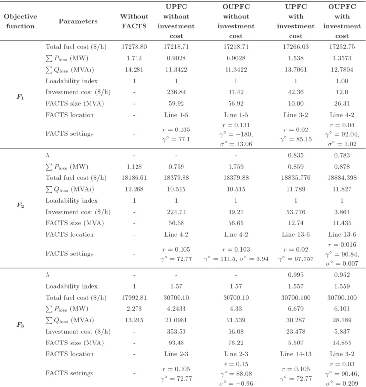
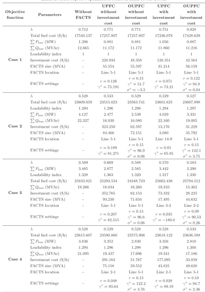
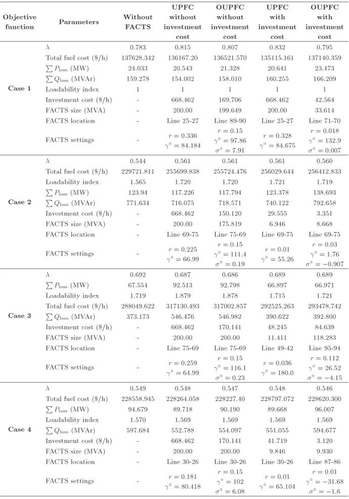
The single-objective and multi-objective optimization problems are performed on IEEE 14-bus test system considering the total fuel cost, active power losses, and the system loadability as objective functions. The results of the single-objective optimization are shown in Table 2 with and without minimization of the investment cost of OUPFC and UPFC devices. In the case without minimization of the investment cost, two devices have a similar performance with dierent sizes while the OUPFC investment cost is less than that of UPFC as much as 80%, 78%, and 81% for optimization of the total fuel cost, active power losses, and the system loadability, respectively. In the case with minimization of the investment cost, OUPFC has better performance than UPFC with 71.1% less investment cost for minimizing the total fuel cost and the investment cost, simultaneously. Also, the UPFC improves investment 2% more than OUPFC to minimize active power losses while the investment cost of UPFC is 92.8% more than that of OUPFC. The results show that utilizing both UPFC and OUPFC enhances system loadability objective function almost equally, but with 75.1% reduction in investment cost of OUPFC compared to that of UPFC.

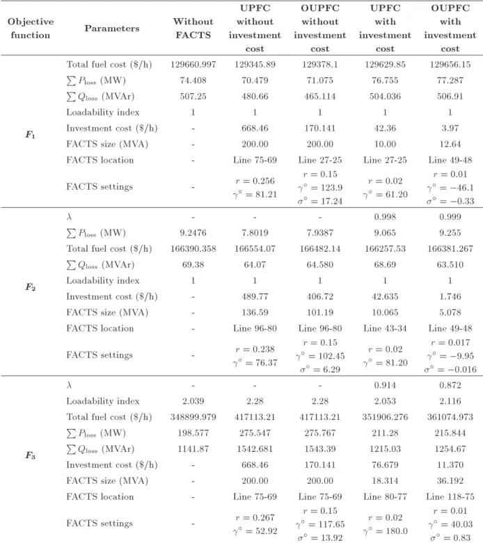
Using fuzzy optimization method in solving dif-ferent combinations of stated objectives, the multi-objective optimization results with the same weighting coecients are tabulated in Table 3. The simulation re-sults indicate better performance of OUPFC compared

(8)

Table 2. Single objective optimization results in IEEE 14-bus system. Objective

function Parameters

Without FACTS

UPFC without investment

cost

OUPFC without investment

cost

UPFC with investment

cost

OUPFC with investment

cost

F1

Total fuel cost ($/h) 17278.80 17218.71 17218.71 17266.03 17252.75 P

Ploss (MW) 1.712 0.9028 0.9028 1.538 1.3573

P

Qloss (MVAr) 14.281 11.3422 11.3422 13.7061 12.7804

Loadability index 1 1 1 1 1.00

Investment cost ($/h) - 236.89 47.42 42.36 12.0

FACTS size (MVA) - 59.92 56.92 10.00 26.31

FACTS location - Line 1-5 Line 1-5 Line 3-2 Line 4-2

FACTS settings - r = 0:135

_{= 77:1}

r = 0:131 _{= 180,}

_{= 13:06}

r = 0:02 _{= 85:15}

r = 0:04 _{= 92:04,}

_{= 1:02}

F2

- - - 0.835 0.783

P

Ploss (MW) 1.128 0.759 0.759 0.859 0.878

Qloss (MVAr) 12.268 10.515 10.515 11.789 11.827

Loadability index 1 1 1 1 1

FACTS size (MVA) - 56.58 56.65 12.74 11.435

_{= 72:77}

r = 0:103 _{= 111:5,}_{= 3:94}

r = 0:02 _{= 67:757}

r = 0:016 _{= 90:84,}

_{= 0:007}

F3

- - - 0.995 0.952

Loadability index 1 1.57 1.57 1.557 1.559

Ploss (MW) 2.273 4.2433 4.33 6.679 6.101

P

Qloss (MVAr) 13.245 21.0981 21.539 30.287 28.189

FACTS size (MVA) - 93.48 76.22 5.507 14.855

_{= 72:77}

r = 0:15 _{= 88:08}

_{= 0:96}

r = 0:105 _{= 72:77}

r = 0:03 _{= 90:46,}

_{= 0:209}

to that of UPFC with lower investment cost. According to Case 1, by placing OUPFC and minimizing its investment cost, the total fuel cost increases about 1.1% and active power losses decrease about 16% compared to that of UPFC, while without minimization of investment cost, both OUPFC and UPFC give the same result. In Case 2, OUPFC improves system load-ability in both modes of with and without minimizing investment cost, i.e. increasing system loadability, but increases the total fuel cost slightly. Also in Cases 3

and 4, OUPFC has greater impact in reducing active power losses and improving all objective functions with lower investment cost compared to that of UPFC.

To illustrate exibility and interactive properties of the proposed algorithm, Case 4 is investigated considering various weighting factors of objective func-tions. In Table 4, it is assumed that the weighting factor of the total fuel cost objective function is in-creased while the other weighting factors are dein-creased through four steps. Consequently, the total fuel cost

(9)

Table 3. Multi-objective optimization results in IEEE 14-bus system. Objective

function Parameters

Without FACTS

cost

Case 1

0.712 0.771 0.771 0.751 0.928

Ploss (MW) 1.296 0.881 0.881 1.056 0.887

P

Qloss (MVAr) 12.665 11.172 11.172 11.860 11.216

FACTS size (MVA) - 55.554 55.597 31.214 56.159

_{= 75:191}

r = 0:15 _{= 51:7}

_{= 3:5}

r = 0:071 _{= 73:21}

r = 0:122 _{= 94:8}

_{= 0:04}

Case 2

0.528 0.533 0.529 0.529 0.527

Total fuel cost ($/h) 23609.059 23515.023 23563.741 23601.625 23607.898

Loadability index 1.294 1.296 1.298 1.294 1.297

P

Ploss (MW) 4.127 2.477 2.539 4.029 3.331

P

Qloss (MVAr) 22.327 16.030 16.080 22.160 19.005

FACTS size (MVA) - 84.466 72.151 3.080 35.792

_{= 81:271}

r = 0:15 _{= 96:9}

_{= 0:06}

r = 0:01 _{= 65:85}

r = 0:15 _{= 122:1}

_{= 3:75}

Case 3

0.589 0.669 0.588 0.570 0.583

P

Ploss (MW) 3.485 2.877 2.585 3.442 2.290

Qloss (MVAr) 19.266 18.034 16.260 19.310 15.362

FACTS size (MVA) - 93.230 71.634 17.495 44.632

_{= 82:515}

r = 0:15 _{= 96:6}

_{= 0:06}

r = 0:035 _{= 180:0}

r = 0:09 _{= 90:53}

_{= 0:26}

Case 4

0.528 0.529 0.528 0.528 0.533

Ploss (MW) 3.836 3.352 2.830 3.356 2.810

P

Qloss (MVAr) 21.095 19.437 17.696 19.341 17.186

FACTS size (MVA) - 75.158 59.552 43.825 49.620

_{= 93:64}

r = 0:15 _{= 122:2}

_{= 3:76}

r = 0:028 _{= 89:19}

r = 0:10 _{= 94:7}

(10)

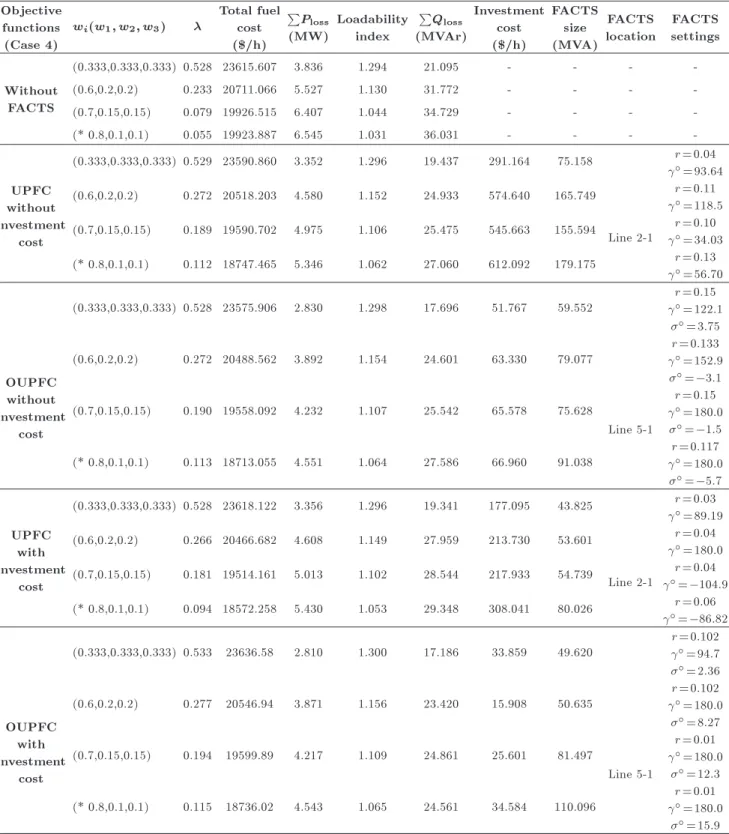
Table 4. Interactive results in Case 4 of IEEE 14-bus system.

Objective functions (Case 4)

wi(w1; w2; w3)

Total fuel cost ($/h)

P Ploss

(MW)

Loadability index

P Qloss

(MVAr)

Investment cost ($/h)

FACTS size (MVA)

FACTS location

FACTS settings

Without FACTS

(0.333,0.333,0.333) 0.528 23615.607 3.836 1.294 21.095 - - -

-(0.6,0.2,0.2) 0.233 20711.066 5.527 1.130 31.772 - - -

-(0.7,0.15,0.15) 0.079 19926.515 6.407 1.044 34.729 - - -

-(* 0.8,0.1,0.1) 0.055 19923.887 6.545 1.031 36.031 - - -

-UPFC without investment

cost

(0.333,0.333,0.333) 0.529 23590.860 3.352 1.296 19.437 291.164 75.158

Line 2-1

r =0:04 _=93:64

(0.6,0.2,0.2) 0.272 20518.203 4.580 1.152 24.933 574.640 165.749 r =0:11 _=118:5

(0.7,0.15,0.15) 0.189 19590.702 4.975 1.106 25.475 545.663 155.594 r =0:10 _=34:03

(* 0.8,0.1,0.1) 0.112 18747.465 5.346 1.062 27.060 612.092 179.175 r =0:13 _=56:70

cost

(0.333,0.333,0.333) 0.528 23575.906 2.830 1.298 17.696 51.767 59.552

Line 5-1

r =0:15 _=122:1

_=3:75

(0.6,0.2,0.2) 0.272 20488.562 3.892 1.154 24.601 63.330 79.077 r =0:133_=152:9

_{= 3:1}

(0.7,0.15,0.15) 0.190 19558.092 4.232 1.107 25.542 65.578 75.628 r =0:15_=180:0

_{= 1:5}

(* 0.8,0.1,0.1) 0.113 18713.055 4.551 1.064 27.586 66.960 91.038 r =0:117_=180:0

_{= 5:7}

cost

(0.333,0.333,0.333) 0.528 23618.122 3.356 1.296 19.341 177.095 43.825

Line 2-1

r =0:03 _=89:19

(0.6,0.2,0.2) 0.266 20466.682 4.608 1.149 27.959 213.730 53.601 r =0:04 _=180:0

(0.7,0.15,0.15) 0.181 19514.161 5.013 1.102 28.544 217.933 54.739 r =0:04 _{= 104:9}

(* 0.8,0.1,0.1) 0.094 18572.258 5.430 1.053 29.348 308.041 80.026 r =0:06 _{= 86:82}

cost

(0.333,0.333,0.333) 0.533 23636.58 2.810 1.300 17.186 33.859 49.620

Line 5-1

r =0:102 _=94:7

_=2:36

(0.6,0.2,0.2) 0.277 20546.94 3.871 1.156 23.420 15.908 50.635 r =0:102_=180:0

_=8:27

(0.7,0.15,0.15) 0.194 19599.89 4.217 1.109 24.861 25.601 81.497 r =0:01_=180:0

_=12:3

(* 0.8,0.1,0.1) 0.115 18736.02 4.543 1.065 24.561 34.584 110.096 r =0:01_=180:0

_=15:9

function approaches its ideal solution value and two other functions are kept out of their ideal solution values.

5.2. IEEE 118-bus test system

The IEEE 118-bus test system is used to examine the performance capability of the proposed algorithm

in locating UPFC and OUPFC, individually, in order to improve objective functions. Single- and multi-objective optimization results are shown in Tables 5 and 6, respectively. Although UPFC has better performances compared to OUPFC in some cases, the OUPFC investment cost is low compared to that of UPFC.

(11)

Table 5. Single objective optimization results in IEEE 118-bus system. Objective

function Parameters

Without FACTS

cost

F1

Ploss(MW) 74.408 70.479 71.075 76.755 77.287

P

Qloss (MVAr) 507.25 480.66 465.114 504.036 506.91

FACTS size (MVA) - 200.00 200.00 10.00 12.64

_{= 81:21}

r = 0:15 _{= 123:9}

_{= 17:24}

r = 0:02 _{= 61:20}

r = 0:01 _{= 46:1}

_{= 0:33}

F2

- - - 0.998 0.999

P

Ploss(MW) 9.2476 7.8019 7.9387 9.065 9.255

Qloss (MVAr) 69.38 64.07 64.580 68.69 63.510

FACTS size (MVA) - 136.59 101.19 10.065 5.078

_{= 76:37}

r = 0:15 _{= 102:45}

_{= 6:29}

r = 0:02 _{= 81:20}

r = 0:017 _{= 9:95}

_{= 0:016}

F3

- - - 0.914 0.872

Ploss(MW) 198.577 275.547 275.767 211.28 215.844

P

Qloss (MVAr) 1141.87 1542.681 1543.39 1215.03 1254.67

FACTS size (MVA) - 200.00 200.00 18.314 36.192

_{= 52:92}

r = 0:15 _{= 117:65}

_{= 13:92}

r = 0:02 _{= 180:0}

r = 0:01 _{= 40:03}

_{= 0:83}

6. Conclusions

Power system optimization is one of the most impor-tant o-line tools in the eld of operation, planning, and control of power systems. This paper made an attempt to nd the optimal location of OUPFC and UPFC devices to simultaneously optimize total fuel cost, power losses, and system loadability as a multi-objective optimization problem to enable power system dispatcher to operate the power system reliably and

economically. The multi-objective optimization prob-lem was performed by a fuzzy interactive approach. The fuzzy method is preferable to common methods of multi-objective optimization since it is able to inter-act with the decision-maker through the optimization process. The proposed algorithm was implemented in GAMS software and solved using CONOPT solver as a DNLP problem. Simulations were performed on IEEE 14-, and 118-bus test systems. Simulation results show that OUPFC is more capable of improving the

(12)

Table 6. Multi-objective optimization results in IEEE 118-bus system. Objective

function Parameters

Without FACTS

cost

Case 1

0.783 0.815 0.807 0.832 0.795

Ploss (MW) 24.033 20.543 21.328 20.641 23.473

P

Qloss (MVAr) 159.278 154.002 158.010 160.255 166.209

FACTS size (MVA) - 200.00 199.649 200.00 33.614

_{= 84:184}

r = 0:15 _{= 97:86}

_{= 7:91}

r = 0:328 _{= 84:675}

r = 0:018 _{= 132:9}

_{= 0:007}

Case 2

0.544 0.561 0.561 0.561 0.560

Total fuel cost ($/h) 229721.811 255699.838 255724.476 256029.644 256412.833

P

Ploss (MW) 123.94 117.226 117.794 123.378 138.693

P

Qloss (MVAr) 771.634 716.075 718.571 740.122 792.658

FACTS size (MVA) - 200.00 175.819 6.946 8.668

_{= 66:99}

r = 0:15 _{= 111:4}

_{= 0:19}

r = 0:01 _{= 55:26}

r = 0:03 _{= 1:76}

_{= 0:907}

Case 3

0.692 0.687 0.686 0.689 0.689

P

Ploss (MW) 67.554 92.513 92.798 66.897 66.971

Qloss (MVAr) 373.173 546.476 546.982 390.622 392.800

FACTS size (MVA) - 200.00 200.00 11.411 118.283

_{= 64:99}

r = 0:15 _{= 116:1}

_{= 0:23}

r = 0:036 _{= 180:0}

r = 0:112 _{= 26:52}

_{= 4:15}

Case 4

0.549 0.548 0.547 0.548 0.546

Ploss (MW) 94.679 89.718 90.190 89.668 96.007

P

Qloss (MVAr) 597.684 552.788 554.097 551.055 594.677

FACTS size (MVA) - 200.00 200.00 9.846 9.930

_{= 80:418}

r = 0:15 _{= 102}

_{= 6:08}

r = 0:01 _{= 65:104}

r = 0:01 _{= 31:68}

(13)

dispatcher's ability to eectively operate power systems compared to UPFC, while the cost of OUPFC is less than the one of UPFC.

References

1. Lashkar Ara, A., Kazemi, A. and Nabavi Niaki, S.A. \Modelling of optimal unied power ow controller (OUPFC) for optimal steady-state performance of power systems", Energy Convers Manage, 52(2), pp. 1325-33 (2011).

2. Parerni, P., Vitet, S., Bena, M. and Yokoyama, A. \Optimal location of phase shifters in the French network by genetic algorithm", IEEE Trans PWRS, 14(9), pp. 37-42 (1999).

3. Singh, S.N. and David, A.K. \A new approach for placement of FACTS devices in open power markets", IEEE Power Eng. Rev., 21(9), pp. 58-60 (2001).

4. Bhasaputra, P. and Ongsaku, W.L. \Optimal power ow with multi-type of FACTS devices by hybrid TS/SA approach", IEEE Proc. on International Con-ference on Industrial Technology, 1, pp. 285-290 (2002).

5. Saravanan, M., Slochana, S.M.R.L., Venkatesh, P. and Abraham, P.S. \Application of PSO technique for optimal location of FACTS devices considering system loadability and cost of installation", IEEE Power Engineering Conference, l, pp. 716-721 (2005).

6. Lashkar Ara, A., Kazemi, A. and Behshad, M. \Im-proving power systems operation through multiobjec-tive optimal location of optimal unied power ow controller", Turkish Journal of Electrical Engineering & Computer Sciences, 21(1), pp. 1893-1908 (2013).

7. Lashkar Ara, A., Aghaei, J., Alaleh, M. and Barati, H. \Contingency-based optimal placement of Optimal Unied Power Flow Controller (OUPFC) in electrical energy transmission systems", Scientia Iranica, 20(3), pp. 778-785 (2013).

8. Hbiabollahzadeh, H., Luo, G.X. and Semlyen, A. \Hydrothermal optimal power ow based on a com-bined linear and nonlinear programming methodol-ogy", IEEE Trans Power Syst., 4(2), pp. 530-7 (1989).

9. Aghaei, J., Gitizadeh, M. and Kaji, M. \Placement and operation strategy of FACTS devices using optimal continuous power ow", Scientia Iranica, 19(6), pp. 1683-1690 (2012).

10. Aoki, K., Nishikori, A. and Yokoyama, R.T. \Con-strained load ow using recursive quadratic program-ming", IEEE Trans Power Syst., 2(1), pp. 8-16 (1987).

11. Stott, B. and Marinho, J.L. \Linear programming for power system network security applications", IEEE Trans Power Appar. Syst., PAS-98(3), pp. 837-848 (1979).

12. Alsac, O. and Stott, B. \Optimal load ow with steady

state security", IEEE Trans Power Appar Syst., PAS-93(3), pp. 745-751 (1974).

13. Sun, D.I., Ashley, B., Brewer, B., Hughes, A. and Tin-ney, W.F. \Optimal power ow by Newton approach", IEEE Trans Power Appar Syst., PAS-103(10), pp. 2864-75 (1984).

14. Santos, A. and Da Costa, G.R. \Optimal power ow solution by Newton's method applied to an aug-mented Lagrangian function", IEE Proceedings-Gener Transm. Distrib., 142(1), pp. 33-36 (1995).

15. Rahli, M. and Pirotte, P. \Optimal load ow us-ing sequential unconstrained minimization technique (SUMT) method under power transmission losses", Electric Power Syst. Res., 52, pp. 61-64 (1999).

16. Yan, X. and Quintana, V.H. \Improving an interior point based OPF by dynamic adjustment of step size and tolerance", IEEE Trans Power Syst., 14(2), pp. 709-17 (1999).

17. Momoh, J.A. and Zhu, J.Z. Improving interior point method for OPF problem", IEEE Trans Power Syst., 14(3), pp. 1114-1120 (1999).

18. Duong, T.L., JianGang, Y. and Truong, V.A. \Ap-plication of min cut algorithm for optimal location of FACTS devices considering system loadability and cost of installation", Electr. Power Energy Syst., 63, pp. 979-987 (2014).

19. Abou El Ela, A.A., Abido, M.A. and Spea, S.R. \Opti-mal power ow using dierential evolution algorithm", Electric Power Syst. Res., 80(7), pp. 878-885 (2010).

20. Nabavi, S.M.H., Kazemi, A. and Masoum, M.A.S.

\Social welfare maximization with fuzzy based genetic algorithm by TCSC and SSSC in double-sided auction market", Scientia Iranica, 19(3), pp. 745-758 (2012).

21. Ippolito, L. and Siano, P. \Selection of optimal number and location of thyristor-controlled phase shifters us-ing genetic based algorithms", IEE Proceedus-ings-Gener Transm Distrib, 151(5), pp. 630-637 (2004).

22. Gitizadeh, M. and Kalantar, M. \Genetic algorithm-based fuzzy multi-objective approach to congestion management using FACTS devices", Electrical Engi-neering, 90(8), pp. 539-549 (2009).

23. Basu, M. \Multi-objective optimal power ow with FACTS devices", Energy Convers Manage, 52(2), pp. 903-910 (2011).

24. Dondo, M.C. and El-Hawary, M.E. \An approach

to implement electricity metering in real-time using articial neural networks", IEEE Trans Power Del., 18(2), pp. 383-386 (2003).

25. Roa-sepulveda, C.A. and Pavez-lazo, B.J. \A solution to the optimal power ow using simulated annealing", Electr Power Energy Syst., 25(1), pp. 47-57 (2003).

26. Gitizadeh, M. and Kalantar, M. \A novel approach for optimum allocation of FACTS devices using

(14)

multi-objective function", Energy Convers Manage, 50(3), pp. 682-690 (2009).

27. Medina, M.A., Das, S., Coello, C.A.C. and Ramrez, J.M. \Decomposition-based modern metaheuristic algorithms for multiobjective optimal power ow -A comparative study", Engineering -Applications of Articial Intelligence, 32, pp. 10-20 (2014).

28. DelValle, Y., Venayagamoorthy, G.K., Mohagheghi, S.J., Hernandez, C. and Harley, R.G. \Particle swarm optimization: Basic concepts, variants and applica-tions in power systems", IEEE Trans Evolutionary Computation, 12(2), pp. 171-195 (2007).

29. Esmaeili Dahej, A., Esmaeili, S. and Goroohi, A. \Multi-objective optimal location of SSSC and STAT-COM achieved by fuzzy optimization strategy and harmony search algorithm", Scientia Iranica, 20(6), pp. 2024-2035 (2013).

30. Guvenc, U., Sonmez, Y., Duman, S. and Yorukeren, N. \Combined economic and emission dispatch solution using gravitational search algorithm", Scientia Iranica, 19(6), pp. 1754-1762 (2012).

31. AlRashidi, M.R. and El-Hawary, M.E. \Application of computational intelligence techniques for solving the revived optimal power ow problem", Electric Power Syst. Res., 79(4), pp. 694-702 (2009).

32. Baykasoglu, A. and Sevim, T. \A review and classi-cation of fuzzy approaches to multi objective opti-mization", International XII Turkish Symposium on Articial Intelligence and Neural Networks-TAINN (2003).

33. General Algebraic Modeling System (GAMS).

<http://www.gams.com> [accessed 27.10.2010].

34. Noroozian, M., Angquist, L., Ghandhari, M. and Andersson, G. \Use of UPFC for optimal power ow control", IEEE Trans Power Del., 12(4), pp. 1629-34 (1997).

35. Abido, M.A. \Optimal power ow using particle swarm optimization", Electr Power Energy Syst., 24(7), pp. 563-71 (2002).

36. Vlachogiannis, J.G. and Lee, K.Y. \A comparative study on particle swarm optimization for optimal steady-state performance of power systems", IEEE Trans Power Syst., 21(4), pp. 1718-28 (2006).

37. Lashkar Ara, A., Kazemi, A. and Nabavi Niaki, S.A. \Multiobjective optimal location of FACTS shunt-series controllers for power system operation plan-ning", IEEE Trans Power Del, 27(2), pp. 481-490 (2012).

38. Lashkar Ara, A., Kazemi, A., Gahramani, S. and Behshad, M. \Optimal reactive power ow using multi-objective mathematical programming", Scientia Iran-ica, 19(6), pp. 1829-1836 (2012).

39. Cai, L.J. and Erlich, I. \Optimal choice and allocation of FACTS devices using genetic algorithm", In

Pro-ceedings on Twelfth Intelligent Systems Application to Power Systems Conference, Lemnos, Greece, pp. 1-6 (2003).

40. Hong-Zhong Huanga, Ying-Kui Gub and Xiaoping

Du \An interactive fuzzy multi-objective optimization method for engineering design", Engineering Appli-cations of Articial Intelligence, 19(5), pp. 451-460 (2006).

41. Wen Zhanga and Yutian Liu \Multi-objective reactive power and voltage control based on fuzzy optimization strategy and fuzzy adaptive particle swarm", Electr Power Energy Syst., 30(9), pp. 525-532 (2008).

42. Edwin Liu, W.H. and Guan, X. \Fuzzy constraint enforcement and control action curtailment in an optimal power ow", IEEE Trans Power Syst., 11(2), pp. 639-645 (1995).

43. Power systems test case archive. <http://www.ee.wa-shington.edu/research/pstca> [accessed 21.01.2008]. Appendix A

OUPFC data

20₂₀_; _{0 r 0:15;}

; XB = 0:007 p.u.;

XE = 0:001 p.u.; Sbase= 100 MVA:

UPFC data

0 r 1 XB= 0:007 p.u:;

XE = 0:001 p.u.; ;

Sbase= 100 MVA:

Biographies

Afshin Lashkar Ara (M'11-SM'15) was born in Tehran, Iran, in 1973. He received his BSc degree in Electrical Engineering from the Islamic Azad Uni-versity, Dezful Branch, Dezful, Iran, in 1995. He received his MSc degree in Electrical Engineering from University of Mazandaran, Babol, Iran, in 2001. He received his PhD degree in Electrical Engineering from Iran University of Science and Technology (IUST), Tehran, Iran, in 2011. He is currently a faculty member in Islamic Azad University, Dezful Branch, Dezful, Iran, as well as a senior member of IEEE Power and Energy Society (IEEE-PES). His current research interests include analysis, operation, and control of power systems and FACTS controllers.

Meisam Shabani was born in Ahwaz, Iran, in 1984. He received his BSc and MSc degrees in Electrical Engineering from the Islamic Azad University, Dezful

(15)

branch, Dezful, Iran, in 2007 and 2011, respectively. His research interests are in power system analysis, fuzzy systems, stability and control, and FACTS de-vices.

Seyed Ali Nabavi Niaki (M'92-SM'04) received the BSc and MSc degrees in Electrical Engineering from Amirkabir University of Technology, Tehran, Iran, in

1987 and 1990, respectively, and the PhD degree in Electrical Engineering from the University of Toronto, Toronto, ON, Canada, in 1996. He joined University of Mazandaran, Babol, Iran, in 1996, as a faculty member. Currently, he is in his sabbatical leave in the University of Toronto, ON, Canada. His current research interests include analysis, operation, and control of power sys-tems and FACTS controllers.