Short-term Debt and Financial Crises:
What we can learn from U.S. Treasury Supply
∗
Arvind Krishnamurthy
Annette Vissing-Jorgensen
First Draft: July 5, 2012
This Draft: March 29, 2013
Abstract
We present a theory in which the key driver of short-term debt issued by the financial sector is the portfolio demand for safe and liquid assets by the non-financial sector. This demand drives a premium on safe and liquid assets that the financial sector exploits by owning risky and illiquid assets and writing safe and liquid claims against those. The central prediction of the theory is that government debt (in practice this is predominantly Treasuries) shouldcrowd outthe net supply of privately issued short-term debt (the private supply of short-term safe and liquid debt, net of the financial sector’s holdings of Treasuries, reserves and currency). We verify this prediction in U.S. data from 1914 to 2011. We take a series of approaches to address potential endogeneity concerns and omitted variables issues: Testing additional predictions of the model (notably that checking deposits should becrowded inby government debt supply), including controls for the business cycle, exploiting a demand shock for safe/liquid assets, and exploring the impact of government supply on the composition of consumption expenditures. We also show that accounting for the impact of Treasury supply on bank money results in a stable estimate for money demand and can help resolve the “missing money” puzzle of the post-1980 period. Finally, we show that short-term debt issued by the financial sector predicts financial crises better than standard measures such as private credit/GDP.
JEL Codes: G12, G2, E44
Keywords: Liquidity, Monetary Aggregates, Financial Institutions.
∗Northwestern University, Kellogg School of Management and NBER, [email protected], and Northwestern University, Kellogg School of Management, NBER, and CEPR, [email protected]. We thank Dean Corbae, Bjorn Eraker, Thomas Phillipon, and participants at seminars/conferences at the ECB, Federal Reserve Board, NBER Summer Institute, LAEF, Wharton Financial Crisis Conference, Wisconsin Money and Asset Markets Conference.
1
Introduction
There is a great deal of short-term debt in the economy. Much of this debt is issued by banks and other financial intermediaries. Banks take deposits. Finance companies issue commercial paper. Broker-dealers and hedge funds borrow by issuing repurchase agreements. The process of securitization throws off short-term debt tranches. Even non-financial firms borrow using short-short-term debt, for example, when such firms issue commercial paper. As is now widely appreciated, the funding structures of financial firms play a role in amplifying financial crises, and there has been much interest in understanding the factors driving the prevalence of short-term debt in the financial sectors’ capital structure. For example, our data suggests that the short-term debt issued by the private sector (what we refer to as net private supply, below), as a ratio to GDP, reached a peak of 99 percent in 2007. This number compares to an average ratio of short-term debt to GDP over the period from 1914 to 2011 of about 66 percent.1
Why is there so much short-term debt in the economy? It is an important fact that banks, across many countries and throughout history, have borrowed predominantly via short-term debt. This fact holds across many different tax regimes. Thus, an explanation relying on the favorable tax treatment of debt cannot be the first-order reason for the predominance of debt. The fact also holds across many different regulatory regimes. For example, during the free banking period of the US in the 19th century, there was no insurance on bank deposits (or lender of last resort) and yet banks carried high leverage. An explanation that relies on government insurance on bank deposits also cannot be the first-order reason for banks’ reliance on short-term debt. See Gorton (2012), and references therein, on the history of short-term debt and banking.
This paper provides evidence for a more primitive rationale for the prevalence of short-term debt, one that plausibly holds across many countries and histories. We show that investors have a large demand for safe and liquid investments, and that short-term debt satisfies this demand. Investors’ demand translates into low yields on short-term debt that is safe and liquid. The financial sector supplies such debt by holding positions in other risky assets (loans, securities, etc.) that is funded by short-term debt. The corporate sector, particularly the high-grade segment, also satisfies this demand by issuing commercial paper. Our evidence supports standard theories of banking that emphasize the special role of banks in transforming risky, illiquid assets into safe and liquid assets (Gorton and Pennacchi (1990), Diamond and Dybvig (1983), and Dang, Gorton and Holmstrom (2010)). The evidence is also consistent with the idea that the shadow banking system played an important role in the production of safe and liquid assets over the last decade (Gorton, Lewellen, and Metrick, 2012).
To arrive at these results, we exploit variation in the supply of government securities. In Krishnamurthy and Vissing-Jorgensen (2012) we showed that Treasury bonds are “money-like” in many respects. We established this by showing that reductions in the supply of Treasury bonds lower the yield on Treasury
1
bonds relative to corporate securities that are less liquid and more risky than Treasury bonds, controlling for the default component of the corporate securities. Section 2 below reviews this evidence and extends it to show that results are similar if Treasury yields are replaced with the interest rate on bank accounts (time and savings deposits), suggesting that bank accounts (a large fraction of the financial sector’s short-term debt) share the safety/liquidity features of Treasuries. Given that, section 3 offers a theoretical equilibrium model to explain how changes in Treasury supply can be expected to affect financial sector short-term debt quantities if both satisfy the safety/liquidity demand of the non-financial sector. The main implication is that Treasury supply should crowd out financial sector short-term debt because the reduction in the yield spreads between risky/illiquid asset and safe/liquid asset brought about by an increase in Treasury supply makes it less profitable for banks to take in deposits in order to invest in riskier, less liquid assets.
To test this main prediction, we construct the supply of government securities, defined as the net supply of Treasuries, reserves and currency by the U.S. Treasury and Federal Reserve (i.e. we subtract out the Federal Reserve’s Treasury holdings from total supply of Treasuries) and study the relation between this government net supply variable and the net private supply of short-term debt. The latter variable is the total of all short-term debt issued by the financial sector net of the financial sector’s holdings of Treasuries, reserves, and currency (and net of any short-term assets but these are tiny in practice). We show that the private net supply variable is strongly negatively correlated with the government net supply. This result, together with the result on the impact of Treasury supply on yield spreads between bank accounts relative to corporate securities, suggests that financial sector short-term debt is special and that the financial sector issues such debt in large part to satisfy the special demand for safe/liquid debt. Moreover, we show that reductions in government supply are correlated with increases in financial sector risky/illiquid loans. The picture that emerges from the data is that of a financial sector that is active in transforming risky/illiquid loans into liquid/low-risk liabilities.
These results are reminiscent of results from a large and older money demand literature. That is, our evidence suggests that financial sector debt is “money-like.” However, the money-demand literature has given prominence to the liquidity features of a certain class of bank liabilities, namely liquid debt such as checking accounts at banks (included in M1). We instead focus on financial sector short-term debt in general. Nonetheless, it is useful to think about different components of financial sector short-term debt because it allows us to derive a second prediction of our framework. A special characteristic of checking accounts is that financial institutions typically back a lot of checking accounts by holdings of Treasuries, likely due to the liquidity properties of Treasuries. We show theoretically that this implies that checking accounts (and thus a standard liquidity aggregate such as M1) should be crowdedin by government supply. We show that this holds up in the data, even if one controls for the standard arguments in a money demand function, i.e. the nominal interest rate and income. The effect of Treasury bond supply on M1 has not been recognized
thus far in the literature. We show that accounting for such a relation can help reconcile some of the puzzling behavior in monetary aggregates since the 1980s (the “missing money” puzzle and the instability of money demand relations). The combined evidence that government supply crowd out the private sector’s net supply of short-term debt but crowds in liquid deposits emphasizes the need for careful analysis of the various components of banks’ balance sheets both theoretically and empirically.
An obvious concern with our results is that they may not be causal and instead driven by either omitted variables or reverse causality. US Treasury supply is driven mainly by wars and the business cycle, and these factors may independently affect the financial sector’s use of short-term debt and the financial sector’s lending to the non-financial sector. For example, if loan demand and the budget deficit had opposite cyclicalities, that could perhaps explain the negative relation between short-term debt (or bank lending) and US Treasury supply. Furthermore, financial sector debt and lending may drive Treasury supply via a banking crisis causing a recession and thus a budget deficit. To address these concerns we take a series of different approaches.
First, one of the main objectives of writing down a model is that we show that some types of short-term debt should be crowded out by government supply while others should be crowded in. It is hard to think of an omitted variables/reverse causality story which would explain this.
Second, we show that the negative relation between financial sector net short-term debt and government supply is unaffected by controlling for recent GDP growth. Essentially that is because government supply has little systematic cyclicality. It increases during recessions but also during wars which (in US history) are expansionary. Furthermore, our main relation is robust to dropping the most problematic years with respect to reverse causality, namely those following financial crisis.
Third, we show that consistent with the model, a positive demand shock for safe/liquid assets has the opposite impact on the financial sector’s net supply of short-term debt. The shock we exploit is the dramatic increase in foreign holdings of Treasuries since the early 1970s. It is hard to think of a story in which the US trade deficits that underlie this build-up of foreign Treasury holdings would also cause an increase in US short-term debt (if anything one would expect the opposite as corporate loan demand in the US would decline as more is produced abroad).
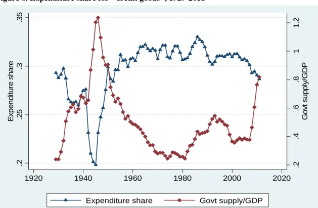
Fourth, we examine the composition of household expenditures. Our model implies that reductions in Treasury supply expand the supply of bank lending. In this scenario, the effective cost (where cost includes financing costs) of goods purchased on credit will fall, leading the expenditure share of such goods to rise. We define goods often purchased on credit to be NIPA categories ”Durable goods” plus ”Housing and Utilities”. We examine this prediction using a widely accepted model of household budget shares, Deaton and Muellbauer’s (1980) almost linear demand system, and confirm the negative relation between Treasury supply and the expenditure share on credit goods. The attractive feature of studying budget shares (as opposed to simply linking bank balance sheets to government supply) is that omitted variables become much
less of an issue when estimating a relation for which there is a standard generally agreed upon framework for which variables should enter as explanatory variables – in this case relative prices and log total real expenditure. This approach resembles that of Rajan and Zingales (1998) who compared the impact of financial development on the relative growth rate of industries who have different dependence on external finance in order to identify the impact of financial development on growth.
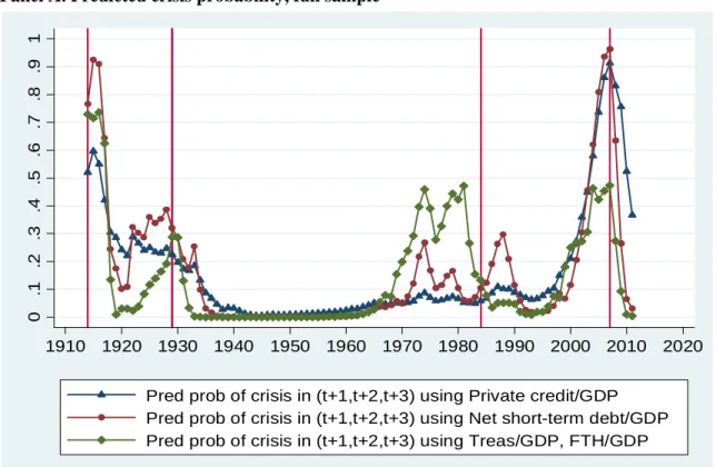
Our last set of results concern predicting financial crises. There is a growing literature that argues that private credit growth, notably growth in bank loans, is a strong predictor of financial crises. Under our banking view, the risk of a financial crisis is primarily driven by the mismatch between the illiquidity/risk of the financial sectors’ assets and liabilities. That is, for predicting crises, it is not loan growth per-se that is important but rather loan growth that is funded by short-term debt. We use our measure of the net private short-term debt supply to predict crises in the U.S. and show that it has more explanatory power than ones based only on loan growth.
The next section of the paper reviews and expands evidence on the impact of Treasury supply on interest rates. Then we lay out a model for understanding the relations between Treasury supply, private demand for short-term liquid and safe debt, and the private supplies of such debt. We then describe how we empirically measure government supply and the private supply variables suggested by the model. Finally, we present our empirical results linking net government supply, private supply, and financial crises. All figures and tables appear at the end of the paper.
2
Price evidence on the moneyness of Treasury bonds and bank
accounts
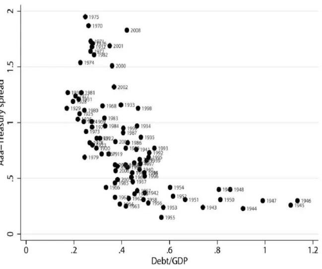
Figure 1 is from Krishnamurthy and Vissing-Jorgensen (2012). The figure graphs the yield spread between Aaa rated corporate bonds and Treasury securities against the US government Debt-to-GDP ratio (i.e. the ratio of the market value of publicly held US government debt to US GDP). The figure reflects a Treasury demand function, akin to a money demand function, that stems from investors’ demand for the high liquidity and safety of Treasuries. We argue in that paper that investors value these money-like features of Treasuries so that when the supply of Treasuries is low, the value that investors assign to the liquidity and safety attributes offered by Treasuries is high. As a result the yield on Treasuries is low relative to the yield on the Aaa corporate bonds which offer less liquidity and safety. Here are the results from that paper which support these conclusions:
1. Table I of the paper shows that the coefficient in a regression of the Aaa-Treasury spread on the log of the Debt-to-GDP ratio, controlling for default risk and default risk premia, is−0.80 (t−stat=−5.12).
Using the Baa-Treasury spread (since Aaa bonds may themselves have some safety properties), the coefficient is−1.31 (t−stat=−7.55).
2. Table I also shows that the coefficient in the regression of short-term commercial paper rates minus Treasury bill rates (high-grade CP minus Bills) on the log of the Debt-to-GDP ratio, after suitable controls, is −0.554 (t−stat=−3.56). Using the spread between lower-grade commercial paper and bills, the coefficient is −1.96 (t−stat=−3.97).
3. Moreover, we show that these effects are driven by investors’ valuation of both the safety and liquidity of Treasury bonds. Table II, column (5), shows that a regression of the spread between 6-month FDIC insured bank CDs and Treasury bills, which is likely a pure measure of the liquidity premium on Treasury bonds, on the log of the Debt-to-GDP ratio, after suitable controls, gives a coefficient of
−1.884 (t−stat=−1.71). Table II, column (4), shows that the regression of short-term low grade commercial paper rates minus high grade commercial paper rates (P2-P1 spread) on the log of the Debt-to-GDP ratio, after suitable controls, gives a coefficient of−0.888(t−stat=−4.34). This spread measures the value of a safe short-term debt investment to investors because P2 rated commercial paper has much lower default risk than P1 rated paper, but has similar transactional liquidity.2
These effects are quantitatively significant. For example a one-standard deviation decrease in the debt-to-GDP ratio from its mean value of 0.44 to 0.24 increases the premium on Treasuries relative to Aaa bonds by 44 basis points. They are also hard to reconcile as an effect on a risk premium using standard CAPM or C-CAPM arguments, so that the liquidity/safety premium arguments we offer in Krishnamurthy and Vissing-Jorgensen (2012) are plausibly the most important factors driving these effects. For example, take the following CAPM logic for these effects. As a set of extreme assumptions to maximize the possible effects, suppose that the correlation between the excess return on Aaa bonds over Treasuries with the return on investors’ overall wealth is one, and that households have no human capital. The risk premium component of the Aaa-Treasury spread is thenσAaa−T reas×γ×σW, where γ is the coefficient of relative risk aversion andσW is the volatility of the representative investors’ wealth. Suppose that the volatility of wealth is given byσW = (1−αT)σrisky+αTσT reasury, whereαT is the fraction of wealth that is Treasury bonds. Moreover, suppose that Treasury bonds are riskless so thatσT reasury= 0, and henceσW = (1−αT)σrisky. Then, the
2
The safety channel is not the same as the risk premium of a standard asset pricing model; it reflects a deviation due to clientele demand. One way to think about investor willingness to pay extra for assets with very low default risk, and to distinguish our explanation from a conventional asset pricing relation between default risk and risk premia, is to plot an asset’s price against its expected default rate. We argue that this curve is very steep for low default rates, with a slope that flattens as the supply of Treasuries increases. This dependence of the price on the supply of long-term Treasuries is how Krishnamurthy and Vissing-Jorgensen (2010) distinguish a standard risk premium explanation of defaultable bond pricing with the clientele-driven safety demand.
risk premium on the Aaa-Treasury spread isσAaa−T reas×γ×(1−αT)σrisky. This model implies that increases in Treasury supply by increasing αT will cause the risk premium to fall. However, quantitatively this effect is likely to be small. Here is a simple calibration. Suppose thatγσrisky = 0.4 which is the Sharpe ratio on the market portfolio. Suppose thatσAaa−T reasis equal to 2%, with the 2% chosen to give a risk premium on the Aaa-Treasury of 80 basis points, which is near the historical average level of this spread. Suppose that
αT is 18% which is approximately the ratio of Treasury supply to total net worth based on Flow of Funds numbers from 2011 (tables B.100 and L.209). Then ifαT falls from 17.6% to 17.6×(0.24/0.44) = 9.6%, the spread would rise byσAaa−T reas×γ×σrisky×∆αT = 200 basis-points ×0.4×(0.176−0.096) which equals 8 basis points and is much smaller than our empirical finding of 44 basis points. Accounting for human capital and a correlation less than one would substantially reduce the effect to be even smaller than the 8 basis points.
The evidence thus suggests the investors have a special demand for liquid and safe assets and that Treasury bonds, because they possess these attributes, have lower yields. The next section of this paper offers an equilibrium model to reconcile this finding. The argument is that reductions in the supply of Treasury bonds reduce a broad aggregate of safe/liquid assets and, given a special demand for safe/liquid assets, reduce the yields on such assets. More interestingly, the model shows that reductions in Treasury supply should increase the supply of private sector assets that are safe/liquid substitutes because such assets also carry a lower yield. Under the hypothesis that financial sector debt is safe/liquid, the theory predicts that the financial sector should issue more safe/liquid debt when Treasury supply falls. This is the central testable implication of our theory that financial sector short-term debt is driven by a demand for safe/liquid assets not captured in standard asset pricing models. We will verify this quantity prediction in the data thus offering insights into to the determinants of the short-term debt funding of the financial sector and the risk of financial crises.
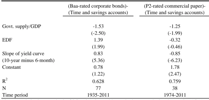
Before turning to the model and the evidence based on quantities it is helpful to first document based on price data that bank accounts share the safety/liquidity features of Treasuries. While it is uncontroversial that checking accounts must have special features (including transactions benefits) in order for them to attract customers despite paying interest rates equal to or close to zero, the same is not obvious for time and savings accounts. These constitute, as we will document in detail below, a larger share of the financial sector’s short-term debt than do checking accounts. In Table 1 we therefore estimate regressions similar to those from Krishnamurthy and Vissing-Jorgensen (2012) but replacing Treasury yields by the interest rate on banks’ time and savings accounts. We calculate the latter based on data from the FDIC’s Historical Statistics on Banking web page. Specifically, we divide the total dollar interest paid on deposits in domestic offices by the dollar amount of time and savings deposits (we use the average of beginning of year and end of year amounts of deposits). We compare this interest rate on time and savings accounts to low-grade
corporate bonds, either long Baa-rated corporate bonds or P1/P2 rated commercial paper. Both corporate yield series are the same as used in Krishnamurthy and Vissing-Jorgensen (2012). We use both a long and a short corporate benchmark since the typical duration of time and savings accounts is unclear. It is shorter than for the long bonds used in the Baa index (which have at least 20 year remaining maturity) and probably longer than for the typical commercial paper, but the exact duration is unclear. To further control for any duration mismatch the regressions include the slope of the yield curve as a control along with a measure of expected corporate default (Moody’s EDF). For consistency with later tables in this paper we use the total government supply/GDP as the main explanatory variable (as detailed below this variable includes the impact of the Federal Reserve), but results are similar if we use Treasury supply/GDP. The regression coefficients of -1.53 and -1.25 are quite similar to those reported above based on yield spreads between corporate securities and Treasuries, suggesting that time and savings accounts are similar in their safety/liquidity features to Treasuries. This is essential for our test of what drives financial sector short-term debt supply to make sense.
3
Model
Time is indexed byt= 0,1. The economy has two classes of agents. Type N agents have a demand for short-term debt while type F has no special debt demand. Furthermore, there is a financial sector that raises equity and debt, makes loans and holds government debt. Assume that type N agents are unsophisticated agents who do not hold bank equity but may hold bank debt, whereas type F agents are sophisticated investors who own all bank equity. In this model, the N agents then reflect the non-financial sector demanders of short-term debt. The F agents reflect the financial sector that supply such debt to the N agents. The modeling omits short-term debt demanders who may also be owners of bank equity.
The government issues Θ units of liquid assets, measured in face value and exogenous to the model.3 We
measure agent N and agent F’s holdings (θN
T and θFT) in units of face value. We solve for the endogenous determination of the financial sector’s supply of short-term debt assets. The diagram below illustrates the relevant balance sheets which we explain in detail next.
3
At this writing of the paper, we do not distinguish between short-term government debt and long-term government debt and treat Θ as the total value of all government debt. We intend to more fully explore the effects of government debt maturity in the next version. Greenwood, Hanson, and Stein (2012) have studied the effects of government maturity structure on financial sector risk within a theoretical model.
F (financial sector) K (Capital) θF T (Treasury Bonds) WF 0 (Equity) DF Deposits - DN θN T N (non-financial sector)
There is a unit measure of N-types who have a special demand for short-term debt. Each N agent maximizes utility function,
max DN,θN T cN0 +v DN 1 +rD + θN T 1 +rT +DN +θNT, (1)
where rD is the interest rate on deposits, rT is the interest rate on government debt, and cN0 is date 0
consumption. The agent purchases deposits and Treasury bonds which payoffDN +θN
T at date 1 and offer an extra utility of v(·) (note that the discount rate is assumed to be zero). The function v(·) takes as argument the market value of debt assets. We assume thatv0(·)>0 and thatv00(·)<0. While we model the
debt demand in reduced form, the literature has noted a number of possible rationales for a demand for short-term debt beyond its simple use for transfering resources to consume later. The money-demand literature motivates a role for checking deposits as a payment medium. The finance literature has motivated a desire for holding a liquid asset to meet unexpected consumption needs of households or unexpected production needs for firms. Krishnamurthy and Vissing-Jorgensen (2012) have shown that there is a demand from investors for “extremely safe” assets (above and beyond what can be rationalized by a CCAPM model) which may be satisfied by short-term financial sector debt as well as Treasury bonds. We first outline the model without taking a stand on the underlying driver of the demand. In the next section, we derive additional predictions of the model based on considerations of the demand for liquid assets.
Agent N’s date 0 budget constraint is,
cN0 + DN 1 +rD + θN T 1 +rT =W0N.
The agent has an initial endowment of wealth WN
0 which we assume to be sufficiently large that in all
equilibria we study the agent is able to setcN
0 strictly above zero.
F-types (financial sector) have no direct debt-demand. Their objective is to maximize,
UF =E[WF 1]− 1 2V ar[W F 1 ], (2)
given an initial endowment of wealthWF
0 . The F-types issue short-term debt to fund a capital investment
that converts one unit of date 0 goods into 1 + ˜r units at date 1, where ˜ris a random variable andE[˜r] =
private sector, which in practice is mainly banks’ corporate loans and mortgage loans. We assume that only the F-types have access to this investment technology. Implicitly we have thus combined the bank with the corporate sector and assumed that banks own the housing stock and rent to households (one could add N-type utility from housing and rent payments to the bank without substantial changes in results).
F types issue debt ofDF, purchase Treasury bonds of θN
T, and invest in capital:
K+ θ F T 1 +rT =W0F + DF 1 +rD .
This results in wealth at date 1 of,
WF 1 = (1 + ˜r)K+θTF−DF = (1 + ˜r)W0F+ DF 1 +rD (˜r−rD)− θ F T 1 +rT (˜r−rT) (3) We allow that WF
1 may be less than zero. That is we do not impose limited liability on the F-types who
are the owners of the financial sector. We do this primarily for simplicity as it ensures that deposits are riskless. More realistically, a model could allow for limited liability and government insurance of deposits. This would introduce risk-shifting incentives as well as a need for government regulation of banks. While these issues are interesting, they do not directly touch on the subject of this paper and are moreover the subject of an extensive literature in banking.
We next solve for equilibrium. Note thatDandθenter the same way into both objective and constraints for both N and F. That is, deposits and Treasuries are perfect substitutes. This observation has two implications. First,rD is equal torT. Second, the equilibrium only pins down net debt holdings ofDN+θNT for N and DF −θF
T for F. This is an important observation because it implies that when considering the short-term debt provided by the financial sector in the data it is important to net out financial sector holdings of Treasury bonds against issued short-term debt.
Consider N’s problem in further detail. The first order condition for choosingDN +θN T is, 1 1 +rD = 1 + 1 1 +rD v0 DN +θN T 1 +rD or, rewriting: −rD=v0 DN +θN T 1 +rD . (4)
Deposits trade at a premium so thatrD<0 (with a sufficiently positive discount rate,rD would be positive but less than the discount rate). Equation (4) is a demand function for debt from N (i.e., −rD is the “convenience yield” cost of buying short-term debt and DN+θNT
1+rD is the purchased amount of debt). Given
our assumptions onv(·), the demand function is downward sloping. F chooses the net debt supply,DF −θF
T, to solve, max DF−θF T E (1 + ˜r)W0F+ DF−θF T 1 +rD (˜r−rD) −1 2 W0F+ DF −θF T 1 +rD 2 σ2r.
The first order condition is, E[˜r−rD]− W0F+ DF −θF T 1 +rD σr2= 0 or, rK−rD= W0F+ DF −θF T 1 +rD σr2 (5)
There is a spread between rK and rD that is increasing in DF −θTF. Equation (5) traces out a supply function for the net debt issued by the financial sector. Note that sincerK is fixed by technology, this first order condition really pins downrD.4
There are two market clearing conditions. First, the deposit market must clear,
DF =DN; second, the Treasury bond market must clear,
θFT +θTN = Θ.
We are interested in understanding how changes in Θ affect equilibrium. Equations (4) and (5) trace out the demand and supply for bank deposits. However, note that the effect of a change in Θ on D is ambiguous. On the one hand, focusing on the demand equation, more Treasury supply could increase θN
T and reduce demand for deposits. On the other hand, focusing on the supply equation, more Treasury supply could increaseθF
T and increase the supply of deposits. The identity of who absorbs the Treasury supply is essential for pinning downD. When we add money demand to the model (see Section 3.1), the model offers some structure on which agents may be expected to absorb the Treasury supply and thus provides additional predictions of the model.
We will approach the problem differently and derive a market clearing condition for the net supply of deposits by the financial sector. Consider thus the equilibrium condition for the overall market for safe/liquid assets. It says that the demand from the non-financial sector must equal the supply from the government plus the net supply of the financial sector
DN +θN T 1 +rD = Θ 1 +rD +D F −θF T 1 +rD . (6)
From equation (4) the non-financial sector’s demand is a decreasing function of−rD since a higher conve-nience yield of buying short-term debt makes this less attractive. From equation (5) the net supply of the financial sector is higher the lower is rD, since this increases the expected return discount on deposits and
4
It is interesting to note that the premiumrK−rDis driven both by the special demand for debt by N (which leads F to
leverage via deposits) and the risk aversion of F. That is, without a special demand for debt, the premiumrK−rDwould be
Treasury bonds, so financial sector net supply is an increasing function of−rD. Let us define the net market value of short-term debt supply issued by the financial sector as,
M = D F −θF
T 1 +rD
.
We will construct this measure from financial sector data. Unlike the case ofD, the determination ofM is unambiguous. The figure below illustrates the equilibrium.
There are two comparative statics that we highlight from this figure:5
• An increase in government supply Θ is a rightward shift in supply that causes the convenience yield,
−rD, to fall andM to fall. The direct impact of the increase in government supply is indicated by the shift from point A to point B in the figure. The indirect effect is to lower the convenience yield on short-term debt (−rD) and thus crowd out private sector net supply, M = DF−θTF
1+rD , moving the
equilibrium from point B to point C.
• An increase in the demand for debt (not illustrated in the figure for readability) is a right shift in the demand schedule and will cause the convenience yield on short-term debt and thus M to rise. Total capital investment of the financial sector can also be related toM:
K=WF
0 +DF/(1 +rD)−θTF/(1 +rT) =W0F+M
5
We can also see that an increase in the volatility of ˜r,σr, is a left-shift in supply, causing the convenience yield to rise and M to fall.
Thus, an increase in Θ decreasesM and reducesK. This is a crowding out effect. If the government supplies more liquidity, the non-financial sector reduces its need for financial sector supplied debt, which reduces funding of the financial sector and reduces lending. Conversely, an increase in the demand for debt increases
M and hence increasesK.
The final measure which is relevant for the analysis is the probability of a financial crisis which we take to be the probability thatWF
1 falls below zero. Rewriting (3),
P rob[WF 1 <0] =P rob (1 + ˜r)WF 0 +M(˜r−rD)<0 (7) Note that total credit, K, does not enter this expression. Total credit is still informative in empirically forecasting crises becauseM =K−WF
0 , and in the data,W0F (i.e. equity) does not vary much. A simple
example to see the difference between K and M is as follows: imagine a bank that has equity of WF
0 and
makes risky loans ofK = WF
0 . Such a bank will never go bankrupt. Thus, it is M rather than K that
should better predict crises in our model. Additionally, more equity, WF
0 , decreases the probability of the
crisis since 1 + ˜r >0. Holding WF
0 and rD constant, the probability of a crisis is increasing in M. There is also a general equilibrium effect onrD which can affect the probability through changing the mean value ofW1F, although
in realistic cases the direct effect ofM is plausibly more significant than the indirect effect. An increase in Θ reducesM and increasesrD. The direct effect reduces the probability of a crisis, while the indirect effect may reduce financial sector profits on average and hence increase the probability of a crisis. An increase in debt demand increases M and reduces rD. The direct effect increases the probability of a crisis, while the indirect effect reduces it. In the summary below, we assume the direct effects dominate.
We summarize the main observations from the model which we will take to the data as follows:
1. In equilibrium, only the financial sector’s net debt supply, M =D−θFT
1+rD, is pinned down.
2. An increase inΘdecreasesM, the debt premium rK−rD, financial sector lending to the private sector,
and the probability of a financial crisis. The effect on the amount of bank deposits (D) and on the size
of the financial sector (D+WF
0)is theoretically ambiguous.
3. An increase in debt demand increases M, the premium, financial sector lending to the private sector,
and the probability of a financial crisis. The effect on the amount of bank deposits (D) and on the size
of the financial sector (D+WF
0)is theoretically ambiguous.
3.1
Money Demand
We next modify the objective (1) to capture money or liquidity demand which is an especially important consideration for bank liabilities. Doing so allows us to clarify how changes in Treasury bond supply interact
with money-demand effects and offers additional predictions of the model.
We divide the N agent into one-half measure of households (NH) and one-half measure of institutional investors (NI). The N household maximizes,
max DNH,θNH T ,LNH cNH0 +µ LNH 1 +rL +v DNH 1 +rD + θNH T 1 +rT + LNH 1 +rL +DNH+θNHT +LNH. (8) Here, LNH are checking/demand deposits paying interest rate rL. The functionµ(·) is a standard money-demand function taking as argument liquid assets that can be used for transactions, unexpected expenditures, etc. The function v(·), as in the earlier specification, is a demand for safe debt so that all of checking accounts, Treasury bonds, and time/saving deposits (DNH) are arguments. We write agent NH’s date 0 budget constraint ascNH 0 + DNH 1+rD + θNH T 1+rT + LNH 1+rL =WNH 0 .
The N institutional investor maximizes, max DNI,θNI T cNI0 +µ θNI T 1 +rT +v DNI 1 +rD + θNI T 1 +rT +DNI+θNIT . (9) subject tocNI 0 + DNI 1+rD + θNI T 1+rT + LNI 1+rL =WNI
0 .The functionµ(·) is also demand for liquid financial assets,
but taking as argument only Treasury bonds. The idea here is that institutional investors (e.g., Microsoft, China) who need to hold a large quantity of liquidity are likely to hold it in Treasury bonds rather than in checking deposits. It is straightforward to mix these objectives and allow each N-type to hold both Treasury bonds and bank deposits with different liquidity valuations of these securities, but the present setup is simpler to exposit.
Consider the NH agent. Following the same analysis as earlier we get the following first order conditions:
−rD = v0 DNH 1 +rD + θ NH T 1 +rT + L NH 1 +rL , (10) rD−rL = µ0 LNH 1 +rL . (11)
The first relation is the same as earlier, taking as argument all debt assets. There is a premium on debt that is short-term but not necessarily liquid (i.e., DNH), given N’s special demand for such debt. The second relation indicates that liquid checking accounts offer an even lower yield because they are valued for their liquidity.
Likewise for the NI agent, we find:
−rD = v0 DNI 1 +rD + θ NI T 1 +rT , rD−rT = µ0 θNI T 1 +rL .
the N sector:6 −rD=v0 DN 1 +rD + θ N T 1 +rT + L N 1 +rL (12) where the quantities with superscript N now refer to the aggregates across the N sector. This demand function is the same as in the model without money demand but incorporating the fact that liquid deposits (L) are also short-term debt and should thus enter the aggregate.
On the financial sector side, we modify the model as follows. We assume that F has to hold some liquid assets in order to be able to meet the liquidity needs that may arise from N possibly withdrawing demand deposits. In particular we require that,
LF 1 +rL ≤ θ F T 1 +rT +κ. (13)
This relation is similar to Bansal and Coleman (1996), where demand deposits are required to be backed by liquid assets. The term κis new and is the amount of capital investment that is liquid. We assume that F can pay a cost Φ(κ) to make some of its capital investment liquid. In practice this may mean investing resources in setting up a repo market against securities, creating a loan sales market, or an asset-backed securities market. With such an investment, F can treat a portion of its K as liquid and use it to back demand deposits. We assume that the function Φ(κ) is increasing and convex with Φ(0) = 0.
With these changes, the budget constraint for F is,
W0F + LF 1 +rL + D F 1 +rD = θ F T 1 +rT +K
and date 1 wealth is,
W1F = (1 + ˜r)K+θTF−DF−LF−Φ(κ). We can substitute from the budget constraint to rewrite date 1 wealth as,
W1F = (1 + ˜r)W0F + DF 1 +rD(˜r −rD) + L F 1 +rL(˜r −rL)− θ F t 1 +rT(˜r −rT)−Φ(κ). Let us define the net debt supply of the financial sector as:
M = L F 1 +rL + D F 1 +rD − θ F T 1 +rT .
Then, the first order condition forDF gives a supply function for net debt supply:
rK−rD= (W0F+M)σ2r (14)
6
That is, first invert the demand curves:
DN H 1 +rD + θ N H T 1 +rT + L N H 1 +rL = v0 −1 (−rD); DN I 1 +rD + θ N I T 1 +rT =v0 −1 (−rD).
The market clearing condition for (overall) deposits now becomes: DN 1 +rD + θ N T 1 +rT + L N 1 +rL = Θ 1 +rT +M
where the left hand side is decreasing in−rD by equation (12) and the right hand side is increasing in−rD by equation (14). Thus, the determination ofM does not change with the addition of money and liquidity demand. The predictions of that analysis continue to hold. Increases in Θ reduce M, reduce the premium on deposits, reduce total lending ofK, and reduce the probability of a crisis.
Let us consider two new predictions arising from the introduction of liquidity demand. First, note that forF, ifrT > rL, F will purchase all of the Treasuries and issue more demand deposits. Thus in an interior equilibrium it must be that7 r
T =rL.This in turn means that we can write the liquidity demand from both N agents in terms of the spread rD−rL:
rD−rL=µ0 LNH 1 +rL and, rD−rL=µ0 θNI T 1 +rT .
Aggregating across the N sector, the demand for liquidity is,
rD−rL=µ0 LN 1 +rL + θ N T 1 +rT . (15)
Turning back to the F agent, the first order condition forκgives,
rK−rL= Φ0(κ) + (W0F+M)σ2r
Liquifying capital costs at the margin Φ0(κ) which in turn allows F to issue more checking deposits and
earn the expected return premiumrK−rL, but at risk cost of (W0F +M)σr2. We can subtract this spread expression from (14) and setrT =rL to write a supply of liquidity function,
rD−rL = Φ0(κ) (16) Equations (15) and (16) can be used to understand bank’s choices over Treasury holdings. The market clearing conditions are, for the checking deposit market:
LN 1 +rL = LF 1 +rL = θ F T 1 +rT +κ
and for the Treasury bond market:
θFT +θTN = Θ.
We combine these conditions to write a market clearing in terms of total liquidity demand from the N sector (left-side) equal to total physical liquidity supply of government bonds plus liquid private capital (right-side):
LN +θN T 1 +rL = Θ 1 +rL +κ (17) 7
It would be easy to modify the model so thatrL< rT as is likely in practice. For example, if we add some administrative
The figure below graphs the market clearing condition (17). The downward sloping line is the demand relationrD−rL=µ0((L+θTN)/(1+rL)). The upward sloping line is the supply relation Θ/(1+rL)+κ, where
κ= Φ0−1(r
D−rL). The figure illustrates the effect of an increase in Θ on the equilibrium. In the figure, such an increase leads to a right-shift in total liquidity supply (the move from point A to point B). This causes the liquidity premiumrD−rL to fall, which by equation (16) crowdsout the financial sectors supply of checking deposits backed by liquid capital,κ(the move from point B to point C). Despite this checking deposits are crowded in by the increases Treasury supply. This is clear from the fact that the NH agents satisfy their demand for liquidity with checking deposits only (not with Treasuries) and the equilibrium liquidity premiumrD−rLhas fallen, thus increasing their liquidity demand (from equation (11)). Similarly,
θN
T rises since it is also decreasing in rD−rL. The increase in checking deposits are made possible by the fact that since rT =rL the financial sector is willing to provide extra deposits backed by Treasuries. Thus, the financial sector changes their backing of deposits such that θFT
κ+θF T = θFT/(1+rT) L/(1+rL) , which we refer to as the financial sector’s deposit coverage ratio, rises with Θ.
The analysis offers the novel insight that an important driver of a monetary liquidity aggregate such as M1 will be the total supply of government debt. This occurs because the supply of deposits is in part driven by the availability of liquid assets such as Treasury bonds, as backing. Moreover, the supply of deposits is driven by both Treasury backing as well as liquid capital. Thus the model further implies that as the supply of Treasuries rises, the financial sector substitutes away from using liquid capital and uses more Treasuries to back the deposit supply.
To summarize, the model with money/liquidity demand offers several more observations which we take to the data:
1. There are two premia arising from investor preferences for debt: (1) a liquidity premium measured as
rD−rT whererD is the interest rate on safe but less liquid debt such as time and savings deposit rate
or commercial paper rates, and rT is the interest rate on liquid Treasury debt; and, (2) a debt premium
measured as rK−rD, where rK is the expected return on an illiquid and risky loan.
2. Increases in Θdecrease bothrK−rD and rD−rT.
3. An increase in Θleads to an increase inL.
4. An increase in Θ leads to an increase in the financial sector’s deposit coverage ratio defined as
θF T/(1+rT)
L/(1+rL).
Note that (1) and (2) are in line with the empirical evidence we have outlined in Section 2 from Krish-namurthy and Vissing-Jorgensen (2012). Thus, we will focus on testing (3) and (4).
4
Empirical framework
We focus on the period from 1914-2011. We begin our analysis in 1914 following the creation of the Federal Reserve System in 1913 in order to avoid any instability in supply or demand functions due to changes in financial sector risk as a result of the Federal Reserve.
The next section explains our data definition of the government’s supply of safe and liquid assets. Section 4.2 explains our empirical framework for constructing the financial sector’s balance sheet and mapping it to the concepts in the model.
4.1
Defining government net supply of safe and liquid assets
We are interested in the government’s supply of safe and liquid assets, Θ. The main component of this is Treasury securities, but to capture the full impact of the government one should also consider the role of the Federal Reserve. We therefore add reserves and currency and security repurchase agreements that are liabilities of the Federal Reserve, but subtract the Federal Reserve’s holdings of Treasuries as well as security repurchase agreements on the asset side of the Federal Reserve’s balance sheet since these are used to back the reserves and currency and thus do not represent securities available for the private sector to hold.8 Our
definition is thus as follows:
8
There are some other categories on both the asset and liability side of the Federal Reserve’s balance sheet, but these are small in most years. The part of government supply coming from the Federal Reserve (reserves+currency+net security repurchase agreements issued by the Federal Reserve-Treasury securities held by the Federal Reserve) average only 5.5 percent
Government sector net supply of safe and liquid instruments (Θ) =Treasuries at market value
+Reserves
+Currency, except for the part held by the Treasury
+Net security repurchase agreements issued by the Federal Reserve
−Treasury securities held by the Federal Reserve
We construct Treasuries at market value as in Krishnamurthy and Vissing-Jorgensen (2012) who construct it based on the book value of Treasuries/GDP from Henning Bohn, multiplied by a market/book adjustment calculated by the authors using data from the CRSP bond database. From 1945 on reserve data are from FoF L.109 line 28, currency from FoF L.109 line 29+35+36+37, net security repos from FoF L.109 line 38-line 9, and Treasuries held by the Federal Reserve from FoF L.109 line 12. We use the FoF release of December 8, 2011. Prior to 1945 we obtain reserves from Banking and Monetary Statistics (1914-1941 Section 3 Table 39, 1941-1970 Section 3 Table 3.1), currency from Friedman and Schwartz (Table 1), and Federal Reserve Treasury holdings from Banking and Monetary Statistics (1914-1941 Section 13 Table 149, 1941-1970 Section 13 Table 13.4). Repurchase agreements were not used by the Federal Reserve during this period. Note that Friedman and Schwartz’s currency measure excludes holdings of the Treasury, consistent with our definition above. However, Friedman and Schwartz’s currency measure also excludes currency holdings of banks. We therefore add bank holdings of currency with data obtained from All Bank Statistics (1959) Table A-1.
4.2
Constructing an overall balance sheet for the U.S. financial sector
We use data on the financial sector from the Flow of Funds Accounts (FoF) from 1952 to 2011. Prior to 1952 we use data from All Bank Statistics (1959) Table A-1.
To test the implications of our model we need to address a series of issues regarding the financial sector. First, the financial sector is increasingly complex, extending far beyond just commercial banks. We need to construct a comprehensive framework to capture all parts of the financial sector including the shadow banking system. Conceptually, in our model F refers to any institution who is a supplier of liquid/safe assets backed by holdings of capital and government bonds. From a certain point of view, one could think that F
of GDP, while our total supply variable averages 47.0 percent of GDP. Conceptually it makes sense that the Federal Reserve’s contribution to the net supply of safe and liquid assets is small. If, as a simple case, the Federal Reserve issued currency and reserves and backed these 100 percent with Treasury securities, then Federal Reserve’s contribution to the net supply of safe and liquid assets would be zero. The part of government supply coming from the Federal Reserve is at its highest (reaching almost 20 percent of GDP) around 1940 due to substantial amounts of reserves and currency being backed by gold. It was less than 1 percent of GDP in 2007 but then increased to about 8 percent as a result of purchases of agency debt and agency MBS purchases financed by reserves under the Federal Reserve’s quantitative easing programs.
is also a liquidity demander since F owns Treasuries. But this is a mistake. The key to identifying F is that F is a net supplier of liquidity/safety, after netting out Treasury holdings. Following this identification, we define the financial sector as the following sectors in the Flow of Funds Accounts, with FoF Table numbers indicated:
L.110 U.S.-Chartered Commercial Banks L.111 Foreign Banking Offices in U.S. L.112 Bank Holding Companies L.113 Banks in U.S.-Affiliated Areas L.114 Savings Institutions
L.115 Credit Unions
L.121 Money Market Mutual Funds L.127 Finance Companies
L.129 Security Brokers and Dealers L.130 Funding Corporations
L.124 Government-Sponsored Enterprises (GSEs) L.125 Agency- and GSE-Backed Mortgage Pools L.126 Issuers of Asset-Backed Securities (ABS) L.128 Real Estate Investment Trusts (REITs)
Prior to 1952 we use data for “All Banks” (i.e. commercial banks and mutual savings banks) from Table A-1 in All Bank Statistics (1959).9
Second, in the model, the bank deposits (D and L) are contracts written between Ns and Fs. In the world, the existence of an interbank market means that Fs also write safe/liquid claims with each other. It is well understood that there are chains of liquid/safe assets and liabilities that Fs write with each other that arise in the interbank market, the repo market, etc. Our model has nothing to say about the amount of these interbank claims so that it would be inappropriate to include the amount of interbank claims in our measure ofM. Interbank claims net to zero within the banking system. We address this by constructing, for each financial instrument, both the total asset and the total liabilitites of the financial sector and then working with the net holdings of that financial instrument. We then sort instruments into those that are net assets and those that are net liabilities for the financial sector, based on averages from 1914-2011 of the ratio (Assets-Liabilities)/GDP.
Third, in practice the financial sector’s holdings of safe and liquid assets supplied by the government are not only Treasuries but also bank reserves and vault cash. We include these in our empirical measure ofθF
T. Fourth, while our model has only two asset categories (Treasuries, risky investments) and three liability
9
categories (checkable depositsL, other deposits D,and equityWF
0 ), the financial sector holds many types
of instruments within each category. A total of 33 different types of instruments show up as an asset and/or liability of one or more of the 14 parts of the financial sector from the FoF listed above (this is after grouping some similar subcatories together). Prior to 1952 (in All Bank Statistics) less detail is available so many of the 33 categories are set to zero. We list the 33 categories in Table 1. The first two are those supplied by the government/Federal Reserve. We group the remaining 31 categories into short-term assets (short-term debt securities not supplied by the government /Federal Reserve), long-term assets (long-term debt securities not supplied by the government/Federal Reserve), and equity-type investments on the asset side and short-term debt (broken into checkable deposits and other short-term debt), long-term debt and equity-type claims on the liability side.
Table 2 shows the resulting financial sector balance sheet. For each instrument we focus on (assets-liabilities)/GDP (or (liabilities-assets)/GDP for instruments that on average are net liabilities) thus taking out cross-holdings within the financial sector. Cross-holdings tend to be large for instruments that on average are net liabilities for the financial sector as shown in Panel B. Notice for example the substantial holdings by the financial sector of money market mutual fund shares, commercial paper, security credit, agency and GSE-backed securities, corporate bonds issued by ABS issuers, and equity (mainly investments by bank holding companies). This makes it clear that considering the financial sector as a whole is important.
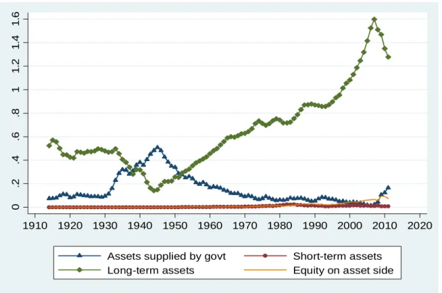
As for the size of the various categories, on the asset side the financial sector is holding substantial amounts of Treasuries as well as cash and reserves, with ratios to GDP averaging 11.2 percent. The other main asset category is long-term assets, mainly mortgages, bank loans and consumer credit. Short-term assets and equity (on the asset side) are very small categories. The overall size of the financial sector relative to GDP averages 81.4 percent, but is much higher in recent years with the latest value at 152.6 percent. Figure 2 Panel A illustrates that the asset side of the financial sector’s balance sheet has fluctuated widely over time. Holdings of assets supplies by the government increased dramatically from 1930 to the mid-1940s but have since declined aside from a spike up in recent years. Long-term assets have followed an opposite pattern. On the liability side of the financial sector’s balance sheet, the vast majority of liabilities are in the form of short-term debt. On average checkable deposits and savings and time deposits are the largest categories, with money market mutual fund shares becoming increasingly important over time. Long-term debt is also becoming increasingly important over time, due mainly to ABS issuer issuing substantial amounts of long-term debt. Figure 2 Panel B illustrates the evolution of the three main categories on the liabilily side. Panel C shows the decomposition of short-term debt into checkable deposits versus other short-term debt. The two sub-components of short-term debt tend to move in opposite directions making the sum look more stable that either of the parts.
correspond well to what we have called risky/illiquid capital (K) in the model. Short-term assets do not map well intoK(since they are unlikely to be either very risky or illiquid). Thus we will subtract them from the short-term debt on the liability side and consider “net short-term debt”, defined as short-term debt minus short-term assets. We also subtract the financial sector’s holdings of assets supplied by the government in our net short-term debt measure consistent with the fact that only the net debt supply,M =D−θTF
1+rD,is pinned
down in the model. As for equity on the asset side, we could consider it part ofK, or net it against the equity on the liability side. We do the latter. On the liability side short-term debt corresponds to L+D (with checkable deposits mapping toLand the other short-term debt categories toD). Long-term debt does not fit well into the model (since it is unlikely that long-term financial sector debt satisfies theN agent’s special demand for very safe assets). Therefore we will subtract them from the long-term debt on the asset side and consider “net long-term investments”, defined as long-term assets minus long-term debt. We note that as shown in Table 2 short-term assets and equity on the asset side are very small and long-term debt is small except for the last couple of decades, suggesting that the main netting issue is not about these categories but about making sure to subtract the financial sector’s holdings of assets supplied by the government in our net short-term debt measure.
Table 3 shows the financial sector balance sheet with short, long, and equity categories netted. Net long-term investments corresponds toK in the model, net short-term debt toL+D−θF
T,and net equity to
WF
0 .Figure 2 Panel D shows the evolution of the three net categories over time. It is clear from this graph
that fluctuations in net long-term investments are driven almost entirely by fluctuations in net short-term debt with equity financing being fairly stable over time.
5
Results
5.1
The impact of government net supply on the financial sector’s net
short-term debt and lending
The predictions of the model regarding the impact of government supply on prices (i.e. spreads) are confirmed in Section 2. The main quantity predictions of the model were:
P1. An increase in Treasury supply Θ decreases the financial sector’s net short term debt M=L+DF−θF
T
1+rD (defined as the financial sector’s short-term debt minus short-term assets minus the financial sector’s holdings of assets supplied by the government).
P2. An increase in Treasury supplyΘdecreases the financial sector’s net long-term investmentsK(defined
Table 4 Panel A and Figure 3 Panel A provide strong evidence in favor of prediction 1 and 2. In Table 4 we estimate regressions of various dependent variables (all scaled by GDP) on government supply/GDP and a trend. Regressions are estimated by OLS but with standard errors adjusted up to account for large positive autocorrelation in the error terms. Based on a standard Box-Jenkins analysis of the error term autocorrelation structure we model the error term as an AR(1) process. One could consider using a GLS estimator (which in many of the regressions would approximately amount to running the regressions in first differences), but as argued by Cochrane (2012) this removes a lot of the most interesting variation in the data. The regression estimates in Table 4 Panel A show that increases in government supply lead to dramatic reductions in the financial sector’s net short-term debt and its net long-term investments, with regression coefficients in both cases around -0.5 and significant at the 1 percent level. The negative relations are apparent in Figure 3 Panel A and seem consistently present over the 98 year period. These results suggest that a one-dollar increase in Treasury supply reduce the net short-term debt issued by the financial sector by 50 cents, and reduce long-term lending of the financial sector by 50 cents.
5.2
Addressing potential omitted variables or reverse causality problems
As laid out in the introduction we take four different (and complementary) approaches to rule out that our main result that government supply crowds out the financial sector’s net short-term debt supply is driven by omitted variables or reverse causality.
5.2.1 Testing additional predictions of the model
One of the objectives of the model was to show that some types of short-term debt should be crowded out by government supply while others should be crowded in. Furthermore, the model predicts that government supply should affect the way the financial sector backs checking deposits. In particular, because of the ability of the financial sector to use Treasuries to back checking deposits the model generated the following additional predictions:
P3. An increase in Treasury supply Θleads to an increase in checkable deposits L.
P4. An increase in Treasury supply Θ leads to an increase in the financial sector’s deposit coverage
ra-tio defined as θTF 1+rT / L 1+rL
(the financial sector’s holdings of assets supplied by the govern-ment/checkable deposits)
A secondary objective of studying checkable deposits is to relate to the literature on money demand and the instability of money demand functions. Many authors have commented on the instability of traditional money demand functions (see Goldfeld and Sichel, 1990). The finding in the literature is that while there
is a stable relation between real money demand M1/P, the nominal interest rate (typically measured as the commercial paper rate), and real income, in the period before 1980, this relation breaks down post-1980. The most prominent puzzle in the literature is the “missing money” of the post-1980 period, when interest rates fell but money balances rose, but not as strongly earlier estimates would have predicted. We will show that accounting for the effects of Treasury supply, as in our model, as well as changes in foreign holdings of Treasuries, can help account for the missing money.
Table 4 Panel C tests prediction 3. Increases in government supply are associated with increases in liquid short-term debt (checkable deposits) with a regression coefficient of about 0.22. Figure 3, Panel B, plots the two underlying series where one can see the positive relation.
Table 4 Panel B shows that increases in government supply leads to an even larger increase in the financial sector’s holdings of government supplied assets, with a regression coefficient of about 0.45. Figure 3 Panel D plots the two series, and one can see the strong positive relation between them. These two results indicate that the financial sector’s deposit coverage ratio is increasing in government supply consistent with prediction 4. This is illustrated in Figure 3 Panel C, which illustrates the positive relation between the government supply and the financial sector’s holdings of government assets divided by checkable deposits. Regressing the deposit coverage ratio on government supply/GDP and a trend results in a coefficient of 1.15 with a t-statistic above 2.
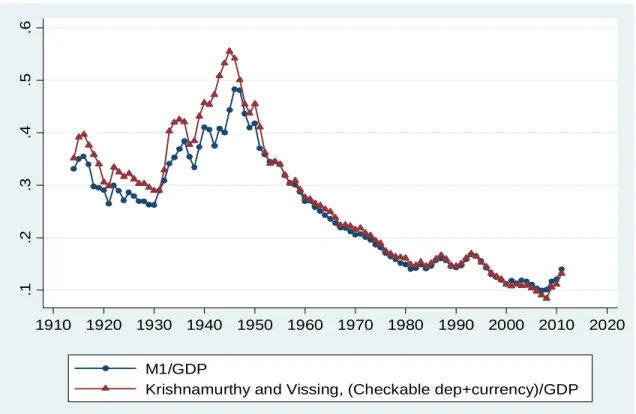
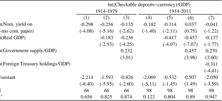
In Table 5 we present estimates of money demand, measured as log of M1/P divided by real GDP (M1 is checkable deposits plus currency), where we include Government supply/GDP as a regressor in addition to the standard regressors of log of nominal yield of the 3-month commercial paper rate and log of real GDP (see e.g. Teles and Zhou (2005)). In Panel A we use data on checkable deposits from our framework plus currency data from Friedman and Schwartz (1970). In Panel B we use data on M1 from Friedman and Schwartz. The two measures of M1 should conceptually be identical absent data issues and they are in fact very close, see Figure 4 Panel A (we will investigate the small difference further in the next draft).10
Before discussing the results, it is worth understanding why Treasury supply may affect money demand and help resolve the missing money puzzle. In our model, money balances for the NH agent is determined byrD−rL. Most papers in the literature setrL equal to zero, but it is typically recognized that this may not be a good assumption. In the period after 1980, financial innovation leads to the creation of checking or near-checking accounts that pay interest. Even in the period pre-1980, non-interest-rate effects such as the density of bank branches which affect the ease of withdrawing cash from a bank account should enter the spread rD−rL (see Kroszner and Strahan, 1999). Thus, it is clear thatrD−rL is mismeasured in money
10
For further comparison with the the literature Figure 4 Panel B compares our measure of the financial sector’s short-term debt other than checking deposits to the difference between M3 and M1. Our measure is highly correlated but a bit larger than M3-M1.
demand estimations and it is possible that such mismeasurement is the source of the instability in money demand. While we do not directly measurerD−rL, our theory suggests that it is driven by Treasury supply. In the missing money period, there is not enough Treasury supply to back more bank deposits, which works against the fall in the level of interest rates by introducing a factor that raisesrD−rL. By accounting for this latter effect, our model helps explain the missing money puzzle.
The comparison of panel A, column (1) and column (4) reveals the standard instability result reported in many other papers: over the period from 1914 to 1979, a money-demand function with a unit income elasticity and interest rate elasticity of−0.3 is a good fit for money demand; over the period from 1914 to 2011, the same regression produces an extremely poor fit for money demand with the regressionR2 falling
from 66% to 12% and interest rate elasticity going from−0.3 to−0.18. TheR2 difference is ameliorated if
we allow for income elasticity different than one, as in column (2) and column (5). But now the estimated elasticities on the interest rate and on income differ considerably over the two samples, again underscoring the instability result.
In columns (3) and (6) we add our government supply variable (in logs to match the left-hand side variable) as suggested by the theoretical model. Government supply is important both in the pre-1980 period and the post-1980 period, as indicated by the significant coefficient estimates on government supply and the substantially higherR2 in column (3) than in column (2) and in column (6) than in column (5).
That is, the fact that the pre-1980 money demand estimates from the literature were stable was lucky, as even over this period the demand function had omitted an important covariate.
In column (7) we also add the log of Foreign Treasury holdings/GDP. We obtain data on Foreign Treasury holdings from FoF L.209 from 1945 on and set the ratio Foreign Treasury holdings/GDP to 0.01 before that when foreign treasury holdings as far as we can determine were negligible (the ratio is around 0.01 in the first years for which FoF data are available). We still using US GDP in the denominator. From our theoretical model, foreign investors’ purchase of the Treasury supply can be thought of as a reduction in the supply of Treasuries to domestic banks and investors (i.e., a reduction Θ). Thus, we may expect a negative coefficient on foreign holdings. On the other hand, an increase in foreign purchases may be correlated more broadly with an increase in foreign demand for US safe/liquid assets. Theory thus does not provide a clear prediction on the magnitude or sign the relation between foreign treasury holdings and money since foreign purchases of US assets have multiple facets. The results in column (7) suggest that the second effect is small in the context of checking accounts. Most important, notice that the coefficient estimates on interest rate, income, and government supply are all very similar over the two samples when comparing column (3) and (7) (Foreign Treasury holdings were small for most of the pre-1980 period so we omit that variable for the pre-1980 sample). In short, adding government supply variables leads to a stable estimate of money demand over the entire sample.
Table 4, Panel B presents the same results using our measures of Federal Reserve and Friedman and Schwartz measures of money. As one would expect based on Figure 4 Panel A, the results are not driven by our construction of money aggregates.
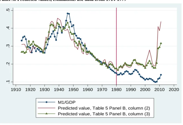
Figure 5 presents the money-demand instability results graphically, focusing on the “missing money” period post-1980. In Panel A, we graph actual M1/GDP along with the predicted value of money based on the specifications of Table 5 Panel B column (2) (allowing income elasticity to differ from one) and column (3) (including government supply). The graph illustrates that the predicted values from column (3) provide a better fit of the data after around 2000, but there is still lots of money missing. Figure 5, Panel B, suggests what is missing. We plot the missing money based on our estimates from column (3) against foreign holdings of Treasury bonds. The two lines show strong trends after around 1980 in opposite directions and of similar orders of magnitude. Figure 5, Panel C shows that the predicted values from column (7), based on the full sample, are very close to the actual ones.
5.2.2 Including controls for loan demand. Dropping observations following financial crisis Our second approach to address potential omitted variables or endogeneity problems concerning the negative relation between government supply and the financial sector’s net short-term debt is to include controls for loan demand and drop observations following financial crisis.
The obvious variable that could, in principle, drive both government supply and net short-term debt is recent economic growth. For example, booms are associated with high loan demand (and thus short-term debt) but low government debt supply. In Table 6 Panel A we include the growth rate of real GDP (based on data from NIPA Table 1.1.6) over the past five years as a control (using a longer or shorter period does not affect the results substantially). Column (1) shows our baseline finding from Table 4 Panel A. Column (2) adds the growth control and column (3) shows the results from the regression without the growth control but estimated over the same sample as column (3). Comparing column (2) and (3) it is clear that including the growth control has essentially no effect on our main result. The lower estimate on government supply/GDP in column (2) than column (1) is entirely driven by the different samples. The underlying reason that including the growth control does not matter is that government supply has little cyclicality on average. It increases during recessions but also during wars which (in US history) are expansionary.
Another potential omitted variables concern is that government spending or taxation may affect loan demand. For example, perhaps high government supply is associated with high current or future taxation, or low current or future government spending, which could depress loan demand. Column (4) includes the (summed) primary deficit over the past 5 years and over the subsequent 5 years as controls, using deficit data from Henning Bohn’s web page. Column (5) estimates the regression without the control but over the same sample period as used in column (4). The negative relation between government supply and the financial