Connected subglacial lake drainage beneath Thwaites Glacier,
West Antarctica
Citation for published version:
Smith, BE, Gourmelen, N, Huth, A & Joughin, I 2016 'Connected subglacial lake drainage beneath Thwaites
Glacier, West Antarctica' pp. 1-19. https://doi.org/10.5194/tc-2016-180
Digital Object Identifier (DOI):
10.5194/tc-2016-180
Link:
Link to publication record in Edinburgh Research Explorer
Document Version:
Publisher's PDF, also known as Version of record
Publisher Rights Statement:
c Author(s) 2016. CC-BY 3.0 License.
General rights
Copyright for the publications made accessible via the Edinburgh Research Explorer is retained by the author(s)
and / or other copyright owners and it is a condition of accessing these publications that users recognise and
abide by the legal requirements associated with these rights.
Take down policy
The University of Edinburgh has made every reasonable effort to ensure that Edinburgh Research Explorer
content complies with UK legislation. If you believe that the public display of this file breaches copyright please
contact [email protected] providing details, and we will remove access to the work immediately and
investigate your claim.
Connected subglacial lake drainage beneath Thwaites Glacier, West
Antarctica
Benjamin E. Smith
1, Noel Gourmelen
3, Alexander Huth
2, Ian Joughin
11Applied Physics Lab, University of Washington, Seattle, WA, 98195, USA
5
2Department of Earth and Space Sciences, University of Washington, Seattle, WA, 98195, USA 3School of Geosciences, University of Edinburgh, Edinburgh, EH8, Scotland
Correspondence to: Benjamin Smith ([email protected])
Abstract. We present conventional and swath altimetry data from Cryosat-2 revealing a system of subglacial lakes that drained between June 2013 and January 2014 under the central part of Thwaites Glacier, West Antarctica. Much of the 10
drainage happened in less than six months, with an apparent connection between three lakes spanning more than 130 km. Hydropotential analysis of the glacier bed shows a large number of small closed basins that should trap water produced by subglacial melt, although the observed large-scale motion of water suggests that water can sometimes locally move against the apparent potential gradient, at least during lake-drainage events, suggesting that there are important limitations in the ability of hydropotential maps to predict subglacial water flow. An interpretation based on a map of the melt rate suggests 15
that lake drainages of this type should take place every 20-80 years, depending on the connectivity of the water flow at the bed. Although we observed an acceleration in the downstream part of TWG immediately before the start of the lake drainage, there is no clear connection between the drainage and any speed change of the glacier.
1. Background
The Amundsen Sea embayment is one of the fastest-changing part of Antarctica, with large changes since at least 20
the 1990s (Rignot, 2008). Increased flow of Thwaites glacier is responsible for around half of the ice-sheet mass loss from this sector (Medley et al., 2014); in response to these large changes, NSF’s AGASEA and NASA’s IceBridge programs have flown extensive surveys measuring ice thickness and bed elevation in this area, with the twin goals of measuring mass-balance changes and enabling accurate ice-flow modeling for the region. As a result, the bed of Thwaites glacier has been mapped in detail, allowing mapping of basal shear stress and potential subglacial water flow paths. These reveal abundant 25
basal meltwater production, estimated at about 3.5 km3yr-1 and averaging ~19 mm yr-1 (Joughin et al., 2009). Melt
production is concentrated in the fast-flowing lower trunk of the glacier, but is locally larger than 20 mm yr-1 even in some
regions within the slow-flowing catchment. Interpretations of radar-reflection properties has also led researchers (Schroeder et al., 2015; Schroeder et al., 2013) to identify an upstream region where water may drain primarily through a distributed network of small pockets, and a downstream region where water may flow through channels. The combination of radar 30
observations and estimated melt rates led to a map of geothermal heat flux, based on the assumption that the basal water system was in equilibrium with steady-state melt rates (Schroeder et al., 2014). Some authors have speculated that changes in this water system could lead to accelerated grounding-line retreat (Schroeder et al., 2013).
Active subglacial lakes (lakes that drain or fill over the course of a few years or less) have been identified throughout Antarctica (Smith et al., 2009). Well-documented lake systems have been observed in slow-flowing ice-sheet 35
tributary regions (Wingham et al., 2006) near ice-shelf grounding lines (Fricker et al., 2007), and around outlet glaciers (Stearns et al., 2008). They are commonly associated with fast-flowing glaciers, where meltwater produced by basal sliding is abundant, and where surface and subglacial topography combine to produce hydropotential features that trap water at the bed (Bindschadler and Choi, 2007).
2
Although active lakes have been identified under many of the large glaciers in Antarctica, none have been found under the Amundsen Coast glaciers (Smith et al., 2009). One explanation for this lack is that the large meltwater production by the fast-sliding glaciers in this region has produced a stable, channelized drainage network that prevents water from accumulating in lakes. An alternate explanation is that the laser-altimetry-based survey that identified lakes in other parts of Antarctica did not make adequate measurements over the cloudy Amundsen Coast to detect the lakes that were there. 5
To overcome the limitations of the existing altimetry record, and to extend the altimetry record nearly to the present day, here we use Cryosat-2 data to map elevation changes on Thwaites Glacier, West Antarctica (Figure 1). Our results show significant water movement beneath the glacier, and imply temporal variability in water flow that is not captured in published models of the glacier.
2. Data and techniques
10
This study combines surface elevation, ice-thickness, and ice-speed data from a variety of sources. We describe each below.
2.1 Surface elevation and elevation-change estimates
The primary source of elevation data for this study are the Cryosat-2 baseline-B radar altimetry data collected between November, 2010 and February 2015, which we refine through a number of steps to derive both POCA (point-of-closest-approach) and swath-mode elevations. With POCA processing, estimates are made of the height and location of the 15
point on the surface that was closest to the satellite when it transmitted a burst of energy, which produces a short-duration, high-energy reflection. Rather than use one of the level-2 retracked products, we apply a maximum-slope retracker to measure the height of these points (Gray et al., 2015), smoothing each waveform with a Gaussian window with a s of 4 samples, and using a threshold of 3.6x10⁻¹⁶W sample-1 to identify waveform-power slopes significantly above the noise
floor, and a coherence threshold of 75%. 20
Like other POCA products, our retracked POCA Cryosat-2 data tend to preferentially measure the heights of local rises on the ice sheet, missing local depressions, which can lead to gaps in the coverage of measurements of up to a few km in the Thwaites Glacier region. To help fill these gaps, we derived additional elevation measurements using a swath-processing strategy to calculate surface heights from the ‘tail’ of the return (Christie et al., 2016; Gray et al., 2013; Hawley et al., 2009), which is energy returned after the POCA. To estimate heights from this part of the waveform, we smoothed the 25
complex phase for each waveform to about 80% of the instrument bandwidth, using a Gaussian kernel with a s of 5 bins, weighted by the coherence values, and calculated a weighted mean of the coherence using the same weights. For most bursts, this resulted in smoothed coherence curves that were high (greater than 75%) over one or more contiguous segments after the POCA points. For any segment longer than 20 bins, we unwrapped the smoothed phase starting at the centre of the segment and, geolocated the measurements for three distinct ambiguity shifts of -2p 0, and 2p. For each segment, we then 30
fit a spline curve to the derived elevations as a function of the across-track distance to the resulting height values with a resolution of 400 m. For each 400-m node in the spline, we calculated the median height (and across-track offset) and RDE (Robust Dispersion Estimate, equal to the half the difference between the 84th and 14th percentiles) of the residuals to the
spline within 200 m of the node. We then compared the median heights to a DEM, and selected the best ambiguity that minimized the median absolute difference of the height residuals for each segment. The swath-height values supplied to our 35
fitting routine are the median-residual elevations (and their locations) around each node, and the errors are the RDEs of the spline residuals.
Swath-processed data over the Thwaites region are affected by metre-scale biases that are correlated over tens of kilometres, and apparently independent from orbit to orbit, possibly because of the time-variable subsurface penetration of radar energy. By combining swath and POCA data, we were able to partially correct for these biases, allowing nearly 40
continuous, dense coverage of our study area. We produced surface-elevation estimates with uniform spacing in space and time using a technique that minimizes the misfit between the irregularly sampled data and a smooth surface-height model that varies in time. In this model, the ice-sheet surface is represented as a digital elevation model (DEM) for June 1, 2011, combined with a set of correction surfaces that map elevation changes between the 2011 DEM and the surface for 3-month increments between 2010 and 2014. This technique minimizes a residual that depends on the roughness of the surface, the 5
spatial variability of the elevation change rate, and the misfit between the surface and the data (Appendix A). With this model, we were able to reconstruct the surface height for our region at any time between mid 2010 and late 2014.
2.2 WorldView photogrammetry elevations
In addition to Cryosat-2, we derived surface DEMs from WorldView optical stereo data processed with ASP, the AMES Stereo Pipeline (Shean et al., 2016). These DEMs have a horizontal resolution of approximately 12 m; experience 10
with these data suggests that each DEM has a uniform bias of around 4 m (RMS), and that correcting for this bias leaves sub-metre vertical errors that are correlated at sub-kilometre scales (Shean et al., 2016). While these data have far finer resolution than Cryosat-2, coverage is much more limited. We constructed a nearly seamless composite DEM for part of our study area from two overlapping pairs of images, both from November of 2014, by correcting for the mean height bias between the two in their overlap area. Two earlier image pairs, from November of 2012 and March of 2013, gave estimates 15
of the surface height for part of the same area, approximately two years earlier.
2.3 Bed DEM
We generated a bed DEM was generated based on the latest available radar-sounding data for the Thwaites region, using a smooth-spline interpolant. As an alternative, we did consider the BEDMAP-2 DEM (Fretwell et al., 2013), but did not use it because it does not include the high-resolution 2012 IceBridge radar-sounding campaign. To derive an estimate of 20
the bed elevation, we used McCords Level-2 (Leuschen et al, 2010) and AGASEA (Blankenship et al, 2012) ice-thickness estimates. Both radar surveys were accompanied by laser-altimetry data sets, so we converted the thickness estimates to bed-elevation estimates by subtracting them from the mean of all laser altimetry measurements within 100 m of the posted thickness estimate location. We used only those radar-sounding estimates collected at altitudes less than 3000 m above the surface.
25
To interpolate a bed DEM from these data, we used an algorithm similar to that used for the Cryosat surface interpolation (Appendix A), solving for a time-invariant bed elevation model. The bed-fitting algorithm included adjustable parameters that controlled the smoothness and the flatness of the interpolated bed, corresponding to parameters Lx in
equation A7 and wx0 in equation A8. A set of constrained, independent parameters allowed for a distinct height bias for each
day on which data were collected, to account for inconsistencies in radar-system parameters and bed-return picking by 30
different operators. The solution gave bias magnitudes less than 6.5 m, 68% of which are less than 2 m; the standard deviation of the difference between the recovered bed DEM and the data points is 11.3 m.
2.4 Hydraulic potential mapping
To help assess the possible water flow at the glacier bed beneath our study area, we mapped the hydraulic potential. This mapping requires surface and bed elevation data.
35
We estimated the hydraulic potential at the bed of the ice sheet as:
4
Here Pw is the water pressure, '% is the density of water g is the acceleration due to gravity, z is the elevation of the glacier
bed above the geoid, and !′ is the hydraulic potential, in units of pressure. If the basal water pressure is equal to the ice overburden pressure, as is commonly assumed, we obtain the glaciological hydraulic potential (Shreve, 1972), which we divided by the unit weight of water to obtain:
! = *+
,-.= ,/
,-)0+
,-1,/
,- )2 , (2)
5
Here '3 is the density of ice, zs is the surface height of the glacier, and !is the hydraulic potential in units of height. We
calculated the hydropotential for our field area using the Cryosat-2 surface height estimate for June 1 2011, combined with a bed DEMs based on radar sounding data; both are measured relative to the EGM-2008 geoid.
If the water pressure at the bed is equal to the overburden pressure, water at the bed will tend to flow along paths parallel to the gradient of !, from high low. This allows the potential map to define the general direction that water paths 10
are likely to follow. We used a D8 routing scheme (for 8-directional, meaning that each pixel routes water to the lowest of its eight neighbours) to calculate the predicted motion of water between nodes in our hydropotential grid (Schwanghart and Scherler, 2014).
At short spatial scales, our potential map contains many locally closed basins. On a bed such as this, long-distance water transport cannot take place unless water can seep through subglacial till, through valleys in the bed too small to be 15
resolved by the radar surveys, or through low-pressure channels that allow water to flow against the local potential gradient. To represent the large-scale basal flow pattern, we ‘conditioned’ our hydropotential map, by artificially filling the closed depressions within each basin to the potential of the lowest point on the boundary, to yield a potential map through which water can steadily flow, because once a basin has been filled, any further water added to it will flow out. Artificially increasing the potential by 1 m is equivalent to raising the bottom of the ice and the surface together by 1 m, or to raising of 20
the bottom of the ice by about 9 m. This conditioning had a similar effect to running a transient water-flow model to steady state before calculating flow paths (Le Brocq et al., 2009) and is among the common strategies used in mapping subaerial flow networks using DEMs that do not resolve the details of every stream valley (Reuter et al., 2009). In some cases, adjacent basins merged during the filling process to form larger, but still closed basins; we continued filling the merged basins until there are no closed contours in the potential map, and used this merged potential map to derive large-scale flow 25
paths.
2.5 Ice-surface velocity mapping
We derived ice-surface velocity maps from a combination of published SAR (Synthetic Aperture Radar) data (Mouginot et al., 2014), feature-tracked LANDSAT data between 2012 and 2016, and TerraSAR-X (TSX) data pairs acquired between July 2011 and August 2014.
30
To investigate possible changes in glacier speed coincident with the elevation changes, we derived speed estimates from Landsat-8 imagery of Thwaites Glacier and surrounding slower-flowing regions. To reduce potential velocity errors due to geometric distortions in the imagery, we tracked only pairs of images collected on the same path and row. This should ensure that errors in feature positions due to inaccuracies in the Landsat geolocation model are nearly the same for both images in a pair, and their errors should cancel in the velocity estimate. We used software based on SAR-speckle-35
tracking algorithms (Joughin, 2002) to estimate offsets between pairs of images and to estimate the contribution of geolocation biases in the images to velocity estimates based on control data on slow-flowing ice.
We also derived velocities for twenty-five periods between June, 2011, and August, 2014, from feature tracking in TSX and TanDem-X image pairs (Tedstone et al., 2014) for an area near the grounding line of Thwaites Glacier. Since there is no exposed rock or truly stagnant ice in these image pairs, in the first instance the image coregistration and 40
feature tracked only image pairs with a minimum of 22 days (2 TerraSAR-X repeat cycles) time-span. To refine the static offsets for each pair, we identified a relatively slowly moving area in the southeast corner of the maps (area C in figure 6) that was well covered in every epoch, and where we assumed that the ice speed was constant. We subtracted the difference between the speed for this area and its mean speed before June 1 2012 from each speed map. We then calculated velocity anomalies for each corrected speed map relative to the pre-june-1-2012 mean speed map. Corrected speed anomalies are 5
mapped in figure S4.
2.6 Subglacial melt-rate estimates
We also used a map of the estimated subglacial melt rate in our area as derived from the surface velocity map, and an estimate of the basal shear stress derived using inverse methods and an ice-flow model (Joughin et al., 2009). This melt-rate estimate does not include the elevated geothermal heat flux that has been hypothesized based on estimates derived from 10
radar (Schroeder et al., 2014), hence it may underestimate actual melt volumes.
3. Results
3.1 Ice-surface elevation and elevation change
The derived June 2011 reference DEM we derived for the Thwaites basin does a good job of resolving kilometre-scale features (see the comparison of surface slope and an optical image mosaic in figure S2). Point-for-point comparison 15
between the DEM elevations and scanning laser altimeter data from 2011 and 2012 shows that the DEM is about 0.6 m higher than the laser data (based on the median difference) with a scatter of about 3 m (based on half the difference between the 16th and 84th percentiles of the distribution). This comparison suggests that the Cryosat-2-based DEM should provide
good estimates of relative height differences across our study area, with local errors on the order of 3 m.
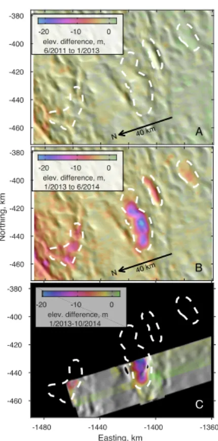
Figure 2A shows the surface elevation change over the 18-month period from June 2011 to January 2013. Overall 20
there was little elevation change over this period. With possible exception of some thinning in the lower left corner, the area shown is far enough upstream that the strong (metres) thinning in response to ice-flow acceleration near the grounding line in the late 1990s and early 2000s (Medley et al., 2014; Mouginot et al., 2014) is not evident. By contrast, Figure 2B shows strong, localized elevation change over the period from January 2013 to June 2014. The most prominent feature in these maps are four general oblong-shaped regions where the surface dropped by many metres. The centres of the features are 25
approximately 70, 124, 142, and 170 km upstream of the grounding line, so we refer to them as Thw70, Thw124, Thw142 and
Thw170. The largest feature, Thw124, is roughly oval, about 16 km wide and 39 km long. Just upstream is Thw142, an
elongated feature about 20 km east-to-west and about 2 km south-to-north. Farthest upstream is Thw170, which extends 11
km south-to-north, and 18 km east-west. The downstream-most feature, Thw70, is angular in shape, with the largest
drawdown concentrated in a region elongated in the NW-SE direction. 30
An independent set of measurements from the Worldview-2 (WV-2) satellites shows the elevation-change pattern for a portion of the western sides of THW124 and Thw70. The November-2014 WV-2 DEM shows the surface height after the
surface change was largely finished. We subtracted the heights measured in the two earlier DEMs, from November 2012 and March 2013, and corrected for residual biases and regional elevation change by subtracting the mean elevation difference outside the boundaries of Thw124 and Thw70. The resulting elevation-change maps (figure 2C) show small (~0.7 m
35
RMS) apparently random elevation variations outside the feature boundaries, up to 20-m subsidence at Thw124, and around
6-m drop at Thw70. The spatial patterns and magnitudes of these changes are both similar to those measured by Cryosat-2.
To derive a volume change for the features, we followed a procedure similar to that used in previous studies of active subglacial lakes (Fricker et al., 2007; Smith et al., 2009). We drew a bounding polygon for each feature that encompasses all substantial (> 0.5 m) elevation change. For each three-month elevation-difference surface, we subtracted 40
6
the elevation change within the polygon from the elevation change in a region between 2 km and 6 km outside the polygon, which corrects for large-scale elevation-change errors, as well as regional drawdown associated with ice-dynamic thinning. Figure 3a shows the mean elevation change with time for each lake. Integrating these corrected changes in space gives the volume change for each feature. Both the elevation and the volume change (Figure 3b) show nearly concurrent drainages. It appears that Thw124, began to deflate first, (January 2013) and continued losing water until mid 2014, with a total loss of 4.5
5
km3. In March 2013, Thw
170 began to drain, and continued until the beginning of 2014, with a total loss of 0.5 km3. Third in
this progression was THW142 draining 0.5 km3 between June of 2013 and January of 2014. Finally, Thw70 lost 0.5 km3,
somewhat more slowly, but primarily between June 2013 and June 2014. The timing of each of these events is somewhat uncertain, because the season-to-season coverage by Cryosat-2 of each feature is inconsistent, and the smoothing constraints applied during the fitting process are expected to yield elevation-change estimates that are temporally smoother than the 10
actual pattern of elevation change; this latter effect is particularly strong at Thw124 because the smoothing constraints tend to
blur the timing of very large changes. As a result, we cannot rule out the possibility that the elevation changes happened at the same time for all four features, or in a different sequence than just described, although the data, taken literally, appear to indicate an earlier change at Thw124.
3.2 Hydropotential maps
15
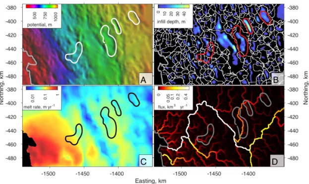
Figure 4A shows the hydropotential map derived for our study area. The surface elevation variations are largely responsible for determining the potential basin shapes, and define distinct basins for each feature. The exception to this pattern is Thw70, which spans a range of hydraulic potentials, with its downstream end about 200 m lower than its upstream
end. Regionally, there is a strong potential gradient driving water parallel to the ice-flow direction, which means that the upstream features have higher potentials than the downstream features. We take the mean potential of the digitized 20
boundary of each feature as representative of the height of the boundary controlling flow into or out of the feature. From upstream to downstream they are 1000, 930, 855, and 715 m, respectively. The differences between the hydropotential map derived from our spline-fit DEM and the BEDMAP-2 DEM (Fretwell et al., 2013) are small, suggesting that our analysis does not depend strongly on the choice of the bed DEM used (see figure S3 for a comparison).
Figure 4B shows the potential difference required to achieve the connected potential map. The merging process 25
(see methods) produced one main basin for each of our drainage features, except for Thw70, which is divided among four.
For most basins, the potential difference is 1-2 m; but for a few, including those associated with Thw124, Thw142, and Thw170,
the potential change required was on the order of 10-20 m. There is also a large area just downstream of, and parallel to, Thw124 that in places required filling by more than 30 m. Figure 4D shows the flow paths calculated from the filled potential
map. This map includes a path that skirts the eastern edges of Thw170 and Thw142, passes through Thw124 from east to west,
30
then sweeps to the northwest, missing Thw70 entirely, and meeting the grounding line approximately in the centre of the
fastest-flowing part of Thwaites glacier. Note that these flow paths and basins are qualitatively the same if we generate a hydropotential map using an alternate data source such as Bedmap-2.
The melt-rate map (figure 4C), combined with the (merged) basin map allow an estimate of the melt-water supply rate to each of our features. First, for each feature, we calculated the rate of melt production within the feature’s local 35
catchment. Next, with the large-scale drainage map, we calculated the rate of melt production over the entire catchment for the feature. These volume rates are reported in table 1.
3.3 Ice-velocity mapping
A profile of speeds for a flowline that runs through our features and out onto the central flowline of the glacier is shown in figure 5, as well as a set of interpolated speeds for a point just downstream of Thw70, and at the grounding line.
40
the grounding line but much smaller 70 km upstream, and scatter in speeds between different sensors, which produces substantial, but not meaningful, apparent speed differences in the velocity-profile plots and in the time-series plots. Any speed change associated with the lake drainage is small compared to the decadal-scale speed variations of the glacier.
A more self-consistent and detailed estimate of speed change around the time of the drainages comes from a set of TSX velocity maps near the grounding line in the fastest part of the glacier (Figure 6, supplemental material figure S4). 5
These maps show that a small area, about 15x20 km in extent, on the east side of the glacier, accelerated by about 100 m yr-1
over the course of the 2013 calendar year. Before this acceleration, this area was slowing at about 50 m yr-2, and after the
start of 2014 it returned to this slowing rate. By contrast, the ice 20 km to the west of the main trunk slowed at about 50 m yr-2 until the start of 2013, then maintained an approximately constant speed through the end of 2014. The centre of the
acceleration feature is within a few kilometres of the drainage channel inferred from the hydopotential maps. 10
4. Discussion
Following previous studies of similar features (Fricker et al., 2007; Gray et al., 2005; McMillan et al., 2013; Smith et al., 2009; Wingham et al., 2006) the simplest and most likely explanation for the observed changes in surface height is the sudden drainage of four subglacial lakes, and we will hereafter refer to the features as lakes. Some authors have suggested, based on airborne-radar observations, that features of this type may in fact reflect the movement of mud or till rather than 15
water (Siegert et al., 2014). We have no strong evidence as the type of material moving beneath the features we observe, although large-scale motion of a 4-km3 volume of a material with significant shear strength (such as till) seems unlikely.
Although some previous studies (Smith et al., 2009) have recommended caution in using coincident filling or draining of adjacent lakes as evidence of hydraulic connection, the nearly simultaneous drainage of four lakes strongly suggests some kind of linkage in the basal hydrological system.
20
4.1 Basal Hydrological System: Linked Lake Catchments
The hydropotential mapping shows that subglacial water flow beneath Thwaites glacier is organized by surface topography into circuitous paths that are often perpendicular to the large-scale flow gradient. The cross-slope water paths are defined primarily by elongated ridges in the glacier surface. Although the bed topography plays a lesser role in defining the flow directions, surface undulations often are muted expressions of features at the bed (Gudmundsson, 2003). Our 25
analysis of the hydropotential maps suggests that together the interaction of bed and surface topography produces a basal hydrologic system that consists of many individual catchments, linked by a series of drainage paths that are at least intermittently active. The bumps at the surface that give rise to the catchments represent large excursions in the driving stress, which is associated with a locally elevated meltwater supply for each catchment. These factors together create an environment favourable to the accumulation of water to form subglacial lakes. Many features do not represent deep sinks in 30
the hydropotential map, so they may simply collect water in a region with little storage, which then cascades downstream to the next catchment. Some of these features, however, represent much deeper sinks in the potential field, which can allow lakes with substantial volume to fill and drain.
Our hydropotential map is not a perfect tool for predicting water flow at the bed since it makes the assumption that the water pressure equals the overburden (i.e., zero effective pressure). Since most sliding laws produce zero resistance with 35
zero effective pressure, at least in some regions the water pressure must be lower than assumed to maintain basal traction, particularly beneath regions where surface slopes are steep (i.e., driving stresses are high). Thus, there is uncertainty our estimates of the details of hydropotential that reflect features and processes that we are unable to resolve with the present data. As a result, while we cannot precisely determine the nature of each flow path from the data, it does appear that some lakes may be connected continuously, while others may have more intermittent connection. In the latter case, only when the 40
8
lakes have filled such that their potential exceeds the minimum local hydropotential barrier do they drain. Note the initial drainage might be slow and inefficient, but once started, a low pressure-gradient channel may develop that leads to more rapid drainage. Once the drainage is complete, without water flow to sustain melting, such a tunnel would close and reseal the lake, allowing it to recharge. Despite these limitations it appears reasonable to assume that lakes form where sinks in the map are the greatest. In fact, the lakes drainages we observe occur precisely where some of deepest closed basins in the 5
hydropotental field exist (Fig 3b). In areas where catchments are connected more continuously without abrupt drainage, water may either move continuously between catchments either through a small network of tunnels or through a less efficient distributed network.
The four lakes appear to have drained nearly concurrently, with Thw124 appearing to precede the others. The upper
three lakes are linked by a through-going potential drainage pathway (Fig. 3d), while Thw70 ties into this drainage pathway
10
farther downstream. As computed, the drainage pathways only exist when the water level rises such that it overcomes the hydropotential barrier. With this model, an upstream lake could overflow into a downstream lake, which would subsequently cause it to overflow, which would then trigger the next event. While this scenario would produce nearly simultaneous drainage, its inconsistent with the observation, which suggest, although not definitively, Thw124 draining first. In principle,
this should not trigger the other lakes, which would have to exceed their own potential barriers. Lowering the potential of 15
Thw124, however, would have forced more water flow toward the lake, at least within the upper confines of its own
catchment. The development of a lower-pressure conduit near the boundary between basins could have altered pressure gradients sufficiently to allow water from the adjacent catchments to spill over, which, through a similar lowering of potential, could have induced drainages of the catchments farther upstream. Perhaps owing to noise in the data or irregular topography, the Thw70 basin is made up of several catchments, some of which are nearly adjacent to the large drainage
20
pathway for the other draining lakes. If this path were closed prior to drainage, but opened to accommodate the Thw124
drainage, then the increased pressure gradient between the channel and Thw70 may have been enough to activate its drainage
pathway.
As just described, lowering the hydropotential gradient at the lower end of a drainage pathway may be sufficient to open it for efficient drainage. This is not a completely satisfying explanation, as some of the pathways are quite long. 25
Nevertheless, it is important to keep in mind the actual water pressure distribution is unknown and evolving with time. Thus, some of the lake may be connected by substantially short paths than shown, with weaker than indicated potential barriers dividing them. Further explanation into the nature of the triggered drainage likely will require a far more detailed hydrological data, likely constrained by a better resolved bed model.
This picture of lakes and subglacial hydrology complicates the modelling of subglacial water flow. Some 30
techniques for estimating subglacial water flow rates (Schroeder et al., 2014) infer the hydraulic conductivity of the glacier bed under the assumption that the conductivity is sufficient to evacuate the meltwater produced steadily by the glacier. Our results show that the instantaneous conductivity at any time may be substantially too small to evacuate the steady meltwater production upstream, but that while lakes are draining, the conductivity increases dramatically. Over the course of multiple lake-drainage cycles, the time-averaged conductivity should be adequate to remove the steady-state melt, but the balance 35
cannot be assumed at any given moment.
From the melt rate estimates and our inferred drainage pathways, we can make some estimates about the recharge times of the lakes. The last two columns of table 1 show the time required for each lake to refill after its observed drainage, based on local and on catchment-scale melt production, ranging from 39 to 83 years for the upper three lakes. If the lakes collect water from upstream catchments, however, this range becomes 4.7 to 22 years. As noted above, the melt estimates 40
assume a fairly low estimate of the geothermal heat flux (Joughin et al., 2009). and the actual value could be significantly higher (Schroeder et al., 2014). As a result, these times could be a few years faster than indicated. The fact that the hydropotential barriers seem low for many catchments favours aggregation of water in a few lake basins with the
correspondingly faster recharge times. This is consistent with the relatively abundant observations of active lakes around Antarctica (Smith et al., 2009).
4.2 Influence of Drainage on Glacier Speed
The sudden injection of a large volume of water under the trunk of an active glacier has in some cases led to a 5
short-term acceleration in flow and discharge (Stearns et al., 2008). For Thwaites Glacier, however, the extra water seems to have had little or no influence on the speed of the lower trunk of Thwaites Glacier. The largest acceleration detected at the grounding line, immediately after the bulk of the drainage was finished, amounted to at most 150 m yr-1, or less than 10% of
the pre-acceleration speed. This is only moderately larger than the longer-term ice-stream speed trend of around 4% yr-1
between 2003 and 2010. Moreover, speedups of this magnitude can also be explained by ungrounding in response to ocean 10
melting (Joughin et al., 2014).
The lack of a strong acceleration in response to the lake drainage should not be surprising. Model-based estimates of the basal shear stress of the lower trunk of Thwaites glacier (Joughin et al., 2009) shows basal drag concentrated in narrow (~5 km wide) bands oriented perpendicular to flow. It seems likely that the glacier speed is largely determined by the drag in the high-stress regions and by lateral shear stress supported outside the lateral margins. If the water discharged 15
from Thw124 moved through narrow channels, it would have occupied only a small area of the bed, and the total change in
force on the glacier, proportional to the product of the area occupied by the channels and the mean shear stress over that area, would likely have been small. Moreover, channels with lower pressure than the surrounding hydrological system might actually withdraw water from higher-pressure distributed systems and act to decrease speeds. Further, the discharge of Thw124 only lasted a few months, so even if it had produced a significant ice-speed change, its effect on the net discharge
20
of the glacier averaged over several years would have been minimal.
5. Conclusions
Our altimetry measurements reveal a substantial (>3.5 km3) short-term transfer of water across the bed of Thwaites
Glacier. Multiple subglacial lakes appear to have drained, with a temporal pattern that suggests linkage over more than 100 km, with a pattern of drainage suggesting that the lakes were connected to a subglacial water system that could change its 25
discharge rate drastically over a few months. Although more than 3 km3 of water appears to have reached the fastest flowing
part of the ice stream over during this time, the added water appears to have had no substantial effect on the ice speed, which is different than what has been reported for some other glaciers (Stearns et al., 2008), but not surprising based on principles of basal-hydrological and basal-sliding theory.
Historically, most full ice sheet models have been developed at resolutions of 10 to 40 km, which is insufficient to 30
resolve topography at the scale that gives rise to the linked catchments shown in Figure 3. Most models have assumed relatively smooth gradients in the hydropotential field that drives an efficient or inefficient drainage network, which is generally driven by bed properties at that scale of mm to m. As we are able to measure the ice sheet surface and bed at ever improving resolution, it is becoming apparent that the routing of basal water is highly dependent on processes acting at the km scale and a linked catchment system represents a different paradigm than has or could be considered in most ice sheet 35
models thus far.
While our data suggest water is routed in ways not presently accounted for in most ice sheet models, it also indicates that the basal hydrological system may not matter much. The basal water system is able to sequester large volumes of water over years which it then releases rapidly with little or no apparent change in glacier speed. This insensitivity suggests that the details of the basal hydrological system may not be the most important feature of the ice sheet for models to 40
10
capture, especially now that data assimilation techniques allow us to infer the dynamic properties of the bed (e.g., the coefficients in a sliding law) directly (Joughin et al., 2010; Morlighem et al., 2010). At least at the decadal scale, fixed bed parameters can reasonably reproduce observed behaviour (Joughin et al., 2010; Joughin et al., 2014), despite large increases in melt production that accompany a speedup and lake drainages. The data are too sparse at present to say definitively whether an evolving hydrological system is an essential part of a predictive ice sheet model. Nevertheless, the data that do 5
exist suggest that such sensitivity to hydrological evolution may be small. Existing satellites such as CryoSat, ICESat, and several SAR missions have already provided a wealth of data to explore such issues. The launch of ICESat-2 (Ice, Cloud Elevation Satellite-2) in late 2017 or early 2018, and the launch of the NASA ISRO SAR (NiSAR) in 2020 will improve this situation considerably.
Appendix A. Methods for estimating elevation and elevation change.
10
Based on the Cryosat data, we estimate elevation changes and a DEM on overlapping 65-km rectilinear grids. Each grid has one set of nodes defining reference DEM heights (for June 1 2011), spaced 500 m in each direction, and one set of nodes defining elevation-change surfaces for 3 month increments between June 1, 2010 and March 1, 2015, spaced at 1 km in each direction. Collectively, the heights of these nodes constitute an elevation model, giving the height of any point within the grids, for any time between the first and last elevation-change surfaces. The centres of individual grids are spaced every 25 15
km, so each grid overlaps its neighbours by 20 km. When the solution is complete, the grids are merged into a master grid using a raised-cosine-taper weighting function that ensures that the master grid elevations and elevation changes are smooth across the grid boundaries.
We solved for the surface heights and elevation changes by minimizing a penalty function, R2, that depends on the
mismatch between the elevation model and the data, and on the spatial gradients in the maps. Selecting a model (a set of 20
surface grids and a set of bias parameters) that minimizes R2 gives the smoothest model consistent with the data, subject to
the choice of trade-off parameters that determine the smoothness of the final model. This penalty function is:
45= 6
3789/,;/>,</=2/17/
/
5 ?@ABA
3CD + 69EF9 )E + 69<F9 GH7G< + 6<<F<< J) + F2K + FH7E J) , (4)
The first term is minimized by reducing the data misfit, equal to the difference between the sum of the surface model, zm(xi,
yi, ti), the bias model, bi, and the measured elevations, zi. The other terms are model constraints that impose a penalty on
25
models that have large slopes or roughness, or that have excessively large biases. The second and third terms are minimized by reducing spatial variations in the DEM height and in the elevation-change rate, fourth term is minimized by reducing the temporal variation in the elevation-change rate at each node, and the last term is minimized when the bias-model parameters are small. Here Fx is an operator that increases with the first and second spatial derivatives of its argument. σi are the estimated data errors, and wi are a set of data weights. The parameters wxo, wxt, and wtt determine the importance of
30
variations in the spatial and temporal derivatives of the model heights, relative to the other residual errors. Fb(b) is a
function of the bias-model parameters (b) that increases with their magnitude and/or roughness and curvature.
The surface model is expressed as a set of nodal values for a DEM, and for a set of quarter-annual correction surfaces. The elevation of any point within the model domain, with spatial coordinates (x,y) at time t, can be found by spatial interpolation between the DEM nodes to give reference DEM height, and by spatio-temporal interpolation into the 35
elevation-difference nodes to give the height difference between the surface June 1, 2011, and the surface at (x,y) and time t:
Here Ixy and Ixyt are operators that interpolate the nodal values to the specified locations. We use a bilinear interpolation in
space, and a cubic-spline interpolation in time; since these are linear operations, we make this calculation using a matrix multiplication:
RS= TUV;W SR (6)
Here zm is a vector of heights interpolated from the model and Ixy;t is a matrix that, multiplied by elevation model mz, gives 5
the height estimates at x, y, and t.
The bias model has one variable for each orbit, nk that gives a bias for swath elevations, one parameter for all
points, kp that gives the height sensitivity to the log of the returned power, and a 2-km geographic grid of values, ksp that
gives a bias between swath and POCA elevations:
K3= XYJ!3+ Z[ log _3 − log _E + P9; M3, N03; Z0[ abc d6eOℎ _bgXOdabc $ijk _bgXOd . (7)
10
As before, Ixy is the operator giving the linear interpolation of the grid points ksp to the measurement points (xi, yi). We can
write this as a matrix multiplication:
l = mSl. (8)
Here B is a matrix calculated based on the power, phase, and location of the data points, b is a vector of bias values calculated from the bias model, and mb is a vector containing nk, kp, and ksp.
15
Using (5) and (7), we can write the first term of (3) as
noS − R pq1r noS − R (9)
Here Gd is the horizontal catenation of Ixy;t and B, and m is the vertical catenation of mzand mb. The remaining terms of (3) help select models that have smoother DEMs, simpler patterns of elevation change, and less complicated bias models. The operator Fx is a discrete approximation of the function
20
F9) = G
s7
G9s
5
+ 2 Gs7
G9G; 5
+ Gs7
G9s
5
uk +D
vsw
G7 G9 5
+ G7
G; 5
uk (10)
When applied to the elevation-change maps, this operator is summed over all pairs of subsequent surfaces. The value of Lx
determines the relative importance of the model gradients and the model curvature to the total residual; it gives the approximate distance over which the surface slope in an unconstrained part of the model approaches zero. We set it to 1 km, the approximate size of gaps between POCA points from distinct tracks in our study area. Discretizing this operator lets us 25
write the second and third terms of (3) as
69E xySzxyS + 69< x{Szx{S . (11)
Here F0 is a discretized version of the gradient of (10) as applied to the DEM, and Fδ is a discretized version of the gradient
of (10) as applied to the elevation-change maps (i.e. the difference between subsequent δz(t) maps).
The fourth term of (3) is minimized by reducing the temporal variation in the rate of elevation change at each node 30
in the δz(t) maps. Ftt(δz) approximates: F<< J) = G
sH7
G<s
5
uO uk. (12)
This operator is discretized on the nodes of δz(t), allowing us to write it as:
xWWSzxWWS. (13)
Here Ftt operates only on the elements of m corresponding to δz. 35
12 The fifth term of (3) minimizes the magnitude of the bias model:
F2= 60[F9 Z0[ +
Y|/
Y|}
?~Ä/BÅ
3CD 5
. (14)
The first term of (14) contributes a larger penalty for larger swath-POCA biases, the second term contributes a larger penalty for larger phase-dependent biases. In matrix notation, the fifth term of (3) is:
xlSl zxlSl. (15)
5
The last term of (3) is used to force the elevation increment for June 1 2011 to be equal to zero. This effectively specifies the date for the DEM:
FH7E= Ç 3ÉÑÖÜá 5EDDJ)35 (16)
Here W is an arbitrary, large weight, which we set to a large enough value that the elevation difference values for June 1 2011 are less than 1 mm. The matrix form of (16) is xH7ES z xH7ES.
10
To solve for the elevation model and bias parameters, we find a model that minimizes R by solving for elevation- and bias-model variables that make the derivative of (3) with respect to the model parameters equal to zero. This leads to a set of linear equations:
no
xy
x{
xWW
xl
x{Ry
Sy
S{
So
+ à = R 0
0 (17)
Here z is a vector of surface-height estimates. We solve this by minimizing the quantity àzâ1Dà, where C is a matrix whose
15
diagonal values give the weights for each component of (3). In principal, this could be solved by standard linear-least-squares techniques (Menke, 1989) but because of the large number of equations and unknowns, we use the Matlab routine lscov, which uses an algorithm designed to efficiently solve large, sparse systems of least-squares equations.
We select weights for our data residuals using the iteratively reweighted least-squares technique(Osbourne, 1985) with a Tukey weighting scheme with a threshold parameter of 3: We calculate the solution initially setting wi=1, then
20
recalculate the weights based on the residuals between the model and the data:
63=
0 ä/
>/ > 3 max (1, í)
1 − ä/
>/Lî9(D,>)
5 5 ä
/
>/ ≤ 3 max (1, í)
(18)
í is a robust estimate of the spread of the scaled residuals with nonzero weight from the previous iteration:
í =D5 $ñó ä
+
>ò − $Dó
ä+
>ò (19)
Here P84() and P14() are the 84th and 14th percentiles of the distribution of the quantity in parentheses. By construction, í =
25
1 for a normalized Gaussian distribution, but outlying residuals affect í less than they would the standard deviation. As we repeat this process over multiple iterations, outlying data are assigned smaller and smaller weights, and the solution converges until either the smallest difference between δz values for two subsequent iterations is less than 0.01 m, or until 20 iterations are complete.
One complication in the iterative-fit procedure is that data with elevations tens of metres from the true surface can 30
produce ‘spikes’ in the DEM that slow the convergence of the entire system. To help eliminate these, when, for a given iteration, the second derivative magnitude for a point in the DEM is greater than 10-4 m-1, all data within 1 km of that point
are removed from the solution at the start of the next iteration. At the end of the next iteration, the solution around the point is usually much smoother, the erroneous data are treated as outliers (with r>3í) in subsequent iterations, and the remaining, non-outlier data around the point are used in the solution.
The selection of the weighting parameters wx0, wxt, and wtt is carried out through a combination of arbitrary choices
and hand tuning. The initial values for each parameter are set based on reasonable values for an ice-sheet, using the 5
formulas:
69ô= k ö G
s7}
G9s
5 1D
69<= k ö G
õH7
G9sG<
5 1D
6<<= k ö G
sH7
G<s
5 1D
(19)
Here A is the domain area and E() is the expected value for a quantity. The normalization ensures that if each quantity in the model is equal to its expected value, the corresponding term in (3) is equal to unity. We began by exploring a range of parameters around the values listed in table 2. The centre of the range for wx0 was chosen based on surface topography with
10
an amplitude of 50 m at a wavelength of 6 km (typical values in an ice-stream environment), the range for the elevation-rate variability parameter is centred on a value chosen based on an 0.1 m yr-1 variation in the elevation-change rate on a 5-km
wavelength. The centre of the range for wtt was chosen based on snow-accumulation-rate variability in the Thwaites
catchment, on the order of 1 m yr-2. For each parameter we tested expected values within 1-2 orders of magnitude of the
centre of the range and evaluated whether each value allowed the inversion procedure to reject outlying data points, while 15
still capturing the pattern of elevation change around Thw124 (Figure S1). The solution is relatively insensitive to variations
in wtt and wx0, with variations around the chosen value by a factor of 30 producing only minor changes in the recovered
pattern of elevation change and the DEM shape. Increasing wtt by more than a factor of 100 (i.e. seeking a much smoother
solution in time) resulted in more severe data editing, and began to degrade the spatial sampling of the solution. By contrast, decreasing wtt by a factor of 10 resulted in a much rougher δz field, while increasing it by a factor of 10 resulted in a blurred
20
map of δz. With our chosen values, the iterative weighting scheme had nonzero weights for about 90% of input data points, and returned a í value of 1.06 m.
A shaded-relief map of the June 1, 2011 surface DEM derived using the selected weights is shown in figure S2. To demonstrate the accuracy of this result, we also show a subset of an optical-image mosaic of Antarctica for the same area. We adjusted the shading azimuth and elevation to achieve a best match between the two, but comparing these maps shows 25
that the DEM captures the few-kilometre-scale surface topography that is visible in the image mosaic.
Author Contributions.
Smith and Gourmellen performed initial altimetry research. Smith developed transient elevation-change and DEM algorithms, and coordinated overall data analysis. Joughin produced Landsat-velocity and melt-rate estimates. Gourmellen produced SAR velocity estimates. Huth developed Cryosat analysis software. All authors contributed to manuscript writing 30
and editing.
Acknowledgments. Work on this paper was funded by NASA grant NNX13AP96G (BS and AH), NSF grant ANT-0424589 (IJ) and European Space Agency’s Support to Science Element programme through CryoTop project 4000107394/12/I-NB and CryoTop Evolution project 4000116874/16/I-NB (NG). DLR project 35
gourmele_XTI_GLAC0296 provided the terrasar-X data. We Acknowledge the support of the Polar Geospatial Center in providing Worldview image data.
14
References
Bindschadler, R. and Choi, H.: Increased water storage at ice-stream onsets: a critical mechanism?, Journal of Glaciology, 53, 163-171, 2007.
Christie, F. D. W., Bingham, R. G., Gourmellen, N., Tett, S. F. B., and Muto, A.: Four-decade record of pervasive grounding line retreat along the Bellingshasuen Margin of West Antarctica, Geophysical Research Letters, 43, 5741-5749, 2016. 5
Fretwell, P., Pritchard, H. D., Vaughan, D. G., Bamber, J. L., Barrand, N. E., Bell, R., Bianchi, C., Bingham, R. G., Blankenship, D. D., Casassa, G., Catania, G., Callens, D., Conway, H., Cook, A. J., Corr, H. F. J., Damaske, D., Damm, V., Ferraccioli, F., Forsberg, R., Fujita, S., Gim, Y., Gogineni, P., Griggs, J. A., Hindmarsh, R. C. A., Holmlund, P., Holt, J. W., Jacobel, R. W., Jenkins, A., Jokat, W., Jordan, T., King, E. C., Kohler, J., Krabill, W., Riger-Kusk, M., Langley, K. A., Leitchenkov, G., Leuschen, C., Luyendyk, B. P., Matsuoka, K., Mouginot, J., Nitsche, F. O., Nogi, Y., Nost, O. A., Popov, 10
S. V., Rignot, E., Rippin, D. M., Rivera, A., Roberts, J., Ross, N., Siegert, M. J., Smith, A. M., Steinhage, D., Studinger, M., Sun, B., Tinto, B. K., Welch, B. C., Wilson, D., Young, D. A., Xiangbin, C., and Zirizzotti, A.: Bedmap2: improved ice bed, surface and thickness datasets for Antarctica, Cryosphere, 7, 375-393, 2013.
Fricker, H. A., Scambos, T., Bindschadler, R., and Padman, L.: An active subglacial water system in West Antarctica mapped from space, Science, 315, 1544-1548, 2007.
15
Gray, L., Burgess, D., Copland, L., Cullen, R., Galin, N., Hawley, R., and Helm, V.: Interferometric swath processing of Cryosat data for glacial ice topography, Cryosphere, 7, 1857-1867, 2013.
Gray, L., Burgess, D., Copland, L., Demuth, M. N., Dunse, T., Langley, K., and Schuler, T. V.: CryoSat-2 delivers monthly and inter-annual surface elevation change for Arctic ice caps, Cryosphere, 9, 1895-1913, 2015.
Gray, L., Joughin, I., Tulaczyk, S., Spikes, V. B., Bindschadler, R., and Jezek, K.: Evidence for subglacial water transport in 20
the West Antarctic Ice Sheet through three-dimensional satellite radar interferometry, Geophysical Research Letters, 32, 2005.
Gudmundsson, G. H.: Transmission of basal variability to a glacier surface, Journal of Geophysical Research-Solid Earth, 108, 19, 2003.
Hawley, R. L., Shepherd, A., Cullen, R., Helm, V., and Wingham, D. J.: Ice-sheet elevations from across-track processing of 25
airborne interferometric radar altimetry, Geophysical Research Letters, 36, 2009.
Joughin, I.: Ice-sheet velocity mapping: a combined interferometric and speckle-tracking approach, Annals of Glaciology, Vol 34, 2002, 34, 195-201, 2002.
Joughin, I., Smith, B. E., and Holland, D. M.: Sensitivity of 21st century sea level to ocean-induced thinning of Pine Island Glacier, Antarctica, Geophysical Research Letters, 37, 5, 2010.
30
Joughin, I., Smith, B. E., and Medley, B.: Marine Ice Sheet Collapse Potentially Under Way for the Thwaites Glacier Basin, West Antarctica, Science, 344, 735-738, 2014.
Joughin, I., Tulaczyk, S., Bamber, J. L., Blankenship, D., Holt, J. W., Scambos, T., and Vaughan, D. G.: Basal conditions for Pine Island and Thwaites Glaciers, West Antarctica, determined using satellite and airborne data, Journal of Glaciology, 55, 2009.
35
Le Brocq, A. M., Payne, A. J., Siegert, M. J., and Alley, R. B.: A subglacial water-flow model for West Antarctica, Journal of Glaciology, 55, 879-888, 2009.
McMillan, M., Corr, H., Shepherd, A., Ridout, A., Laxon, S., and Cullen, R.: Three-dimensional mapping by CryoSat-2 of subglacial lake volume changes, Geophysical Research Letters, 40, 4321-4327, 2013.
Medley, B., Joughin, I., Smith, B. E., Das, S. B., Steig, E. J., Conway, H., Gogineni, S., Lewis, C., Criscitiello, A. S., 40
McConnell, J. R., van den Broeke, M. R., Lenaerts, J. T. M., Bromwich, D. H., Nicolas, J. P., and Leuschen, C.: Constraining the recent mass balance of Pine Island and Thwaites glaciers, West Antarctica, with airborne observations of snow accumulation, Cryosphere, 8, 1375-1392, 2014.
Menke, W.: Geophysical data analysis: discrete inverse theory, Academic Press, San Diego, CA, 1989.
Morlighem, M., Rignot, E., Seroussi, H., Larour, E., Ben Dhia, H., and Aubry, D.: Spatial patterns of basal drag inferred 45
using control methods from a full-Stokes and simpler models for Pine Island Glacier, West Antarctica, Geophysical Research Letters, 37, 2010.
Mouginot, J., Rignot, E., and Scheuchl, B.: Sustained increase in ice discharge fromthe Amundsen Sea Embayment, West Antarctica, from1973 to 2013, Geophysical Research Letters, 41, 1576-1584, 2014.
Osbourne, M.: Finite Algorithms in Optimization and Data Analysis, Chichester ; New York : Wiley, 1985. 50
Reuter, H. I., Hengl, T., Gessler, P., and Soille, P.: Preparation of DEMs for Geomorphometric Analysis. In: Geomorphometry: Concepts, Software, Applications, Hengl, T. and Reuter, H. I. (Eds.), Developments in Soil Science, Elsevier Scientific Publ Co, Po Box 211, 1000 Ae Amsterdam, Netherlands, 2009.
Rignot, E.: Changes in West Antarctic ice stream dynamics observed with ALOS PALSAR data, Geophysical Research Letters, 35, 5, 2008.
55
Schroeder, D. M., Blankenship, D. D., Raney, R. K., and Grima, C.: Estimating Subglacial Water Geometry Using Radar Bed Echo Specularity: Application to Thwaites Glacier, West Antarctica, Ieee Geoscience and Remote Sensing Letters, 12, 443-447, 2015.
Schroeder, D. M., Blankenship, D. D., and Young, D. A.: Evidence for a water system transition beneath Thwaites Glacier, West Antarctica, Proceedings of the National Academy of Sciences of the United States of America, 110, 12225-12228, 60
Schroeder, D. M., Blankenship, D. D., Young, D. A., and Quartini, E.: Evidence for elevated and spatially variable geothermal flux beneath the West Antarctic Ice Sheet, Proceedings of the National Academy of Sciences of the United States of America, 111, 9070-9072, 2014.
Schwanghart, W. and Scherler, D.: Short Communication: TopoToolbox 2-MATLAB-based software for topographic analysis and modeling in Earth surface sciences, Earth Surface Dynamics, 2, 1-7, 2014.
5
Shean, D. E., Alexandrov, O., Moratto, Z., Smith, B. E., Joughin, I. R., Porter, C., and Morin, P.: An automated, open-source pipeline for mass production of digital elevation models (DEMs) from very-high-resolution commercial stereo satellite imagery, ISPRS Journal of Photogrammetry and Remote Sensing, 116, 101-117, 2016.
Shreve, R. L.: Movement of water in glaciers, Journal of Glaciology, 11, 205-214, 1972.
Siegert, M. J., Ross, N., Corr, H., Smith, B., Jordan, T., Bingham, R. G., Ferraccioli, F., Rippin, D. M., and Le Brocq, A.: 10
Boundary conditions of an active West Antarctic subglacial lake: implications for storage of water beneath the ice sheet, Cryosphere, 8, 15-24, 2014.
Smith, B. E., Fricker, H. A., Joughin, I. R., and Tulaczyk, S.: An inventory of active subglacial lakes in Antarctica detected by ICESat (2003-2008), Journal of Glaciology, 55, 573-595, 2009.
Stearns, L. A., Smith, B. E., and Hamilton, G. S.: Increased flow speed on a large East Antarctic outlet glacier caused by 15
subglacial floods, Nature Geoscience, 1, 827-831, 2008.
Tedstone, A. J., Nienow, P. W., Gourmelen, N., and Sole, A. J.: Greenland ice sheet annualmotion insensitive to spatial variations in subglacial hydraulic structure, Geophysical Research Letters, 41, 8910-8917, 2014.
Wingham, D. J., Siegert, M. J., Shepherd, A., and Muir, A. S.: Rapid discharge connects Antarctic subglacial lakes, Nature, 440, 1033-1036, 2006.
20
Lake dV, km3 local melt, km3yr-1 total melt, km3yr-1 T
local, yr Ttotal, yr
Thw70 0.87 0.034 0.07 25 13
Thw124 3.7 0.045 0.17 83 22
Thw142 0.54 0.014 0.12 39 4.7
Thw170 0.49 0.0076 0.044 64 11
Table 1. Discharge estimate for each lake, as well as the local (within-basin) and total (within-basin + upstream) melt supplies to each lake, and the time required for local and total melt supplies to refill the water discharged during the lake drainage.
25
Values considered Value chosen
ö ú5)E
úM5
1.5×101†°1D… 1.5×101£°1D 3×101†°1D Nc1D
ö ú
§J)
úM5úO
1.5×101ñ°1DNc1D… 1.5×101•°1DNc1D 6×101ñ°1D Nc1D
ö ú
5J)
úO5
0.01 ° Nc1D… 10 ° Nc1D 1 m yr-2
16
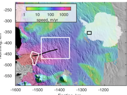
Figure 1. Location map, showing an image mosaic (Scambos and others, 2007) and surface speed (Rignot and others, 2011). White box indicates areas mapped in figure 2, white irregular outline indicates areas mapped in figures 6 and S3. Black line indicates flow line referenced in figure 5. Northing and Easting are in a polar stereographic projection with a standard latitude of -71 S.
-1600 -1500 -1400 -1300 -1200
Easting, km -550
-500 -450 -400 -350 -300 -250
Northing, km
1 10 100 1000
Figure 2. Elevation and elevation change for a study area around Thwaites Glacier. A: Elevation changes between June 2011 and January 2013. B: Elevation changes between January 2013 and June 2014. C. Elevation change recovered from Worldview DEM differencing. Dashed outlines show feature boundaries.
5
Figure 3. Top: Mean elevation change within the digitized outlines, corrected for elevation change outside the outlines as a function of time. Bottom: Calculated volume change within the outlines.
C
-1480 -1440 -1400 -1360
Easting, km -460
-440 -420 -400 -380
-20 -10 0
elev. difference, m 1/2013-10/2014
N 40 km A
-460 -440 -420 -400 -380
-20 -10 0
elev. difference, m, 6/2011 to 1/2013
N 40 km B
-460 -440 -420 -400 -380
Northing, km
-20 -10 0
elev. difference, m, 1/2013 to 6/2014
-6 -5 -4 -3 -2 -1 0
mean height change, m
THW170 THW142 Thw124 Thw70
2011 2012 2013 2014
Year
-4 -3 -2 -1 0
Volume change, km
18
Figure 4. A: Hydropotential map derived from the June, 2011 surface elevation map and our basal topography map. B: Merged basins derived from the hydropotential map, and the water-filling depth required to eliminate local water sinks. C. Melt-rate estimate. D. Water-flux magnitude derived from the basal-melt map and the filled hydropotential map.
5
Figure 5. Glacier surface speeds along a profile running from the grounding line through the draw-down features, plotted as a function of distance upstream of the grounding line. Insets show speeds as a function of time at the downstream end of Thw70,
-20 0 20 40 60 80 100
distance upstream of grounding line, km
0 500 1000 1500 2000 2500 3000 3500
speed, m/a
1995 2005 2015
year
1200 1400 1600 1800 2000
speed at 0 km, m/a
250 300 350 400
and at the grounding line. Lines are colour coded by time, with the complete range of colours shown in the grounding-line (0-km) speed-vs-time plot.
Figure 6. Detail showing speed change at the grounding line, based on Terrasar-X and TanDEM-X SAR velocities. Upper left: the mean speed between mid 2011 and late 2012. Upper right: Speed difference between the August 27, 2013 speed map, and the
5
2011-12 mean speed. The grey line indicates the position of the velocity profile in figure 5. Bottom: Speed change relative to the 2011-12 mean, for two regions, marked ‘A’ and ‘B’. Data from region C were used to correct speed offsets as a function of time. The grey bar indicates the time range of the lake drainage.
2011 2012 2013 2014 2015
year -100
-50 0 50 100 150 200
speed difference, m yr
-1
A
B C
-1540 -1520 -1500
Easting, km
-500 -490 -480 -470 -460 -450 -440
Northing, km
1 2 3
mean speed, km yr-1
-1540 -1520 -1500
Easting, km
-200 0 200