Vol 62, No 3 (2019)

TECHNICAL UNIVERSITY OF CLUJ-NAPOCA

ACTA TECHNICA NAPOCENSIS

DYNAMIC ANALYSIS OF TWO-LINK FLEXIBLE MANIPULATOR USING

FEM UNDERGOING BENDING-TORSIONAL VIBRATIONS

Natraj MISHRA, S.P. SINGH

Abstract- In this paper, a two-link flexible manipulator is analyzed using finite element approach whose links are undergoing combined bending and torsional vibrations. Mathematical model of the flexible manipulator is obtained using Lagrangian dynamics. The links are modelled as Euler-Bernoulli beams and discretized using ‘space-frame’ and ‘plane-frame’ elements. The present work deals with various non-linear effects like, coupling between rigid and flexible degrees of freedom, centrifugal and Coriolis effects and presence of gravity. The mathematical model is validated using results available in the literature. The novelty of the present work lies in inclusion of torsional effects and thus highlighting their effects on positional accuracy of the flexible manipulator.

Keywords- Lagrangian-FEM, coupled bending-torsion vibrations, coupled rigid and flexible motions, Flexible manipulator, frequency analysis

1. INTRODUCTION

Accurate modelling and control of flexibility in robots is a challenging task. Many researchers are working towards achieving the positional accuracy of such robots. If these unwanted vibrations are reduced then definitely, less inertia torque will be required to drive them. This will ultimately lead to the reduction of power consumption by the motors used to drive them. A comprehensive literature review has been done by Benosman and Vey [1]

and Dwivedy and Eberhard [2] in the area of

flexible robotics. They have compiled various

research papers dealing with the modelling and control of flexible robots. Many researchers

have contributed towards area of flexible

robotics. Most of them have used Lagrangian dynamics for modelling the flexible

manipulators. They have treated the links of

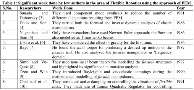
the manipulator as Euler-Bernoulli beams. Table 1 highlights the contribution of these researchers in chronological order.

Table 1: Significant work done by few authors in the area of Flexible Robotics using the approach of FEM

S.No. Researchers Work Done Year

1 Sunada and

Dubowsky [3] They used component mode synthesis to reduce the number of differential equations resulting from FEM. 1981 2. Dado and Soni

[4]

They carried both the forward and inverse dynamic analyses of elastic manipulators.

1986 3. Nagnathan and

Soni [5]

Only these researchers have used Newton-Euler approach; the links are also modelled as Timoshenko beams.

1986 4. Usoro et al. [6] They have considered the effect of gravity for the first time. 1986 5. Bayo [7] He found the joint torque for producing a desired tip motion of the

flexible link. He also analysed the flexible manipulator in ‘frequency domain’.

1987

6. Simo and

Vu-Quoc [8] They used non-linear beam theory for modelling the flexible structures and highlighted its significance in transient analysis. 1987 7. Tzou and Wan

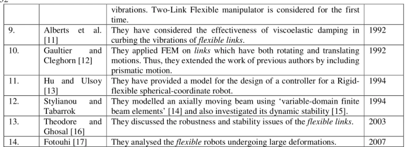
[9] They introduced Rayleigh’s and viscoelastic dampings during the mathematical modelling of flexible manipulators. 1990 8. Chedmail et al.

vibrations. Two-Link Flexible manipulator is considered for the first time.

9. Alberts et al.

[11] They have considered the effectiveness of viscoelastic damping in curbing the vibrations of flexible links. 1992 10. Gaultier and

Cleghorn [12] They applied FEM on motions. Thus, they extended the work of previous authors by including links which have both rotating and translating prismatic motion.

1992

11. Hu and Ulsoy

[13] They have provided a model for the design of a controller for a Rigid-flexible spherical-coordinate robot. 1994 12. Stylianou and

Tabarrok

They modelled an axially moving beam using ‘variable-domain finite beam elements’ [14] and also investigated its dynamic stability [15].

1994 13. Theodore and

Ghosal [16]

They discussed the robustness and stability issues of the flexible links. 2003 14. Fotouhi [17] They analysed the flexible robots undergoing large deformations. 2007 A comparison between the ‘assumed modes

method’ (AMM) and the ‘finite elements method’ (FEM) for modelling flexible multi-link manipulators was done by Meghdari and

Ghassempouri [18] and Theodore and Ghosal [19]. They concluded that the use of FEM is recommended for manipulator links with

complex geometries and having flexibilities and the use of AMM for manipulator links with

uniform geometries.

2. MATHEMATICAL MODELLING

An accurate dynamic model of a Two-link Flexible manipulator having two revolute

joints undergoing both small bending and

small torsional deformations is prepared. Fig. 1 shows a Two-Link Flexible manipulator undergoing both bending and torsional deformations along with rigid revolutions at

their joints. Plane X-Y is the plane of bending

while plane Y-Z is the plane of torsion.

Fig. 1: Dynamic analysis of Two-Link Flexible manipulator undergoing both bending and torsional deformations. In figure 1, X-Y-Z is the reference/ ground

frame while X1-Y1-Z1 and X2-Y2-Z2 are the

local frames attached to Link-1 and Link-2 respectively. Axis X1 is aligned along the

un-deformed neutral axis (N.A.) of Link-1 while axis X2 is aligned along the un-deformed

neutral axis of Link-2. The origins of these local frames are located at Joint-1 and Joint-2 respectively. Joint-1 is given a rigid rotation of θ1 and Joint-2 is given a rigid rotation of θ2.

The position of any point on Link-1 with respect to ground is given by:

= + (1)

Similarly, the position of any point on Link-2 with respect to ground is given by:

= ∗ ₊ ∗ ∗ ₊

∗ ₊

(2) In above expressions,

= cossin −sin 0

0 cos0 01 ;

= cossin −sin 0

= ( , ) 0 ";

∗ _{= # ($ , )}$

0 %; = ( , )0 ";

∗₌ cos(

∗&_{) − sin(} ∗&_{) 0}

sin( ∗&₎

0 cos(

∗&₎

0 01 ;

' = 0 (')' (' ′ ;

' ∗ = 0 (')'∗ (' ′ ;

+ &_{= 0 + 0 ;}

' =

1 0 0

0 cos )' − sin )'

0 sin )' cos )'

;

_' ∗ ₌ 10 cos )0 '∗ − sin )0 '∗

0 sin )'∗ cos )'∗

; (3)

L1 and L2 = lengths of Link-1 and Link-2

respectively,

θ1 and θ2 = joint rotations (rigid) of Joint-1and

Joint-2 respectively,

x1 and x2 = distances measured along

un-deformed Link-1 and Link-2 axes, i.e. X1 and

X2 respectively,

w1(x1, t) and w2(x2, t) = elastic displacements

of Link-1 and Link-2 respectively undergoing bending vibrations

∗&_{= bending angle at end point of Link-1 =} ,-.∗

,/.

{r1} = position coordinates of any point on

Link-1 w.r.t to un-deformed Link-1 axis i.e., X1 in plane X1-Y1

{r2} = position coordinates of any point on

Link-2 w.r.t to un-deformed Link-2 axis i.e., X2 in plane X2-Y2

{r1*} = position coordinates of end point of

Link-1 w.r.t. un-deformed beam-1 axis X1 in

plane X1-Y1

{riT} = position coordinates of any point on

Link-i in plane Yi-Zi

ϕi = ϕi(xi, t) = torsional deformation of any

point on Link-i

ϕi* = ϕi(Li, t) = torsional displacement of end

point of Link-i; i represents the link number (i

= 1 and 2)

The total kinetic energy of the manipulator system is given by:

0. 2. = 3 4 58. 6 & _{6 7}

9 +

3 4 58: 6 & _{6 7}

9 (4)

Total potential energy of the manipulator system is given by:

;. 2. = <.=._{5 >}?:-.:

?/.:@ 7 +

8.

9

A.B._{5 >}?C.

?/.@

8.

9 7 +

3 4 5 + ′8.

9 7 +

<:=:_{5 >}?:-::

?/:: @ 7 +

A:B:

8:

9 5 >?C?/::@

8:

9 7 +

3 4 5 + ′8:

9 7 (5)

In equations- 4 and 5, J1 and J2 are the polar

moment of inertias of Link-1 and Link-2 respectively. The joint torques can be obtained

using Lagrangian dynamics as follows:

, ,D>

?ℒ ?F6@ −

?ℒ

?F = G (6)

In above expression, ℒ represents Lagrangian of the system and is obtained by taking the difference of total kinetic energy and total potential energy of the system; q represents

generalized coordinates and F represents

generalized torque/force.

H =

∗ ∗ _{) )}∗ _{) )}∗ &

(6a)

G = I I 0 0 0 0 0 0 0 0 &

(6b)

3. DISCRETIZATION USING FINITE ELEMENTS METHOD

In this paper, FEM is used to model the vibratory motions of the flexible links. This

involves division of flexible links into some

finite number of elements and finding the inertia and stiffness matrices that govern the dynamics of the system under consideration. Figure 2 (provided at the end) shows the discretization of flexible links using two

Q6i-4 and Q6i-3) and three rotational (Q6i-2, Q6i-1

and Q6i). The complete equation of motion of

the flexible manipulator is given by equation

(7a).

JK_KLL KLM

ML KMMN_{(OPQ) R (OPQ)}SH LT

HMT U_{(OPQ) R} +

J0_{0 0}0_MMN

(OPQ) R (OPQ)V

HL

HMW_{(OPQ) R (OPQ)} +

XY0Z(OPQ) R + X[0Z(OPQ) R = SG L

GMU_{(OPQ) R}

(7a) In equation (7a), subscripts- r and f stand for rigid and flexible respectively. N represents the rigid degrees of freedom present in the system

and n represents the flexible degrees of

freedom obtained from finite element formulation. For the present case, since there are two flexible links, we have N = 2. Hence,

Mrr consists of two diagonal elements- M11 and

M22. Mrf and Mfr represent the coupling

between rigid and flexible motions.

KML = KLM& (7b)

One finite element per link is considered for

the present analysis. Thus, there are three nodes and eighteen degrees of freedom (i.e., n = 18). The first six degrees of freedom are considered to be fixed. Hence, there remain only twelve degrees of freedom. Thus, we get

KMM = \] R (7c)

If there are two finite elements per link then

there will be four elements in total having five nodes. The total degrees of freedom will be thirty then (i.e., n = 30). In the similar fashion, we can obtain the elements of stiffness matrix also. For the present case,

0MM = ^] R (7d)

GL = V_{I W}I (7e)

τ1 and τ2 represent joint torques.

For vibration analysis of the flexible links, it is

necessary to find out the Global stiffness matrix and Global mass matrix. The equation of motion for undamped vibrations for ‘n’ degrees of freedom is as follows:

_KMM`<sub>O×O</sub>bHTMc<sub>O×</sub> + _0MM`_O×ObHMc_O× =

bGMc_O× (8a)

where, Mff = global mass matrix,

Kff = global stiffness matrix,

Ff = global force vector, and

qf = vector of global degrees of freedom.

If damping is present within the system, then the equation of motion for vibratory motion will be written as follows:

_KMM`<sub>O×O</sub>bHMT c<sub>O×</sub> + _dMM`_O×ObHM6 c_O× +

_0MM`_O×ObHMc_O× = bGMc_O× (8b)

where, Cff = global damping matrix.

In local frame, the stiffness matrix of a Space-frame element is given by:

^]& = J^ ] & _^

] &

^& ] ^& ]N (8c)

^& ] =

⎣ ⎢ ⎢ ⎢ ⎢ ⎡4h₀ 0 0 0 0 0 ij 0 0 0 (j 0 0 ik 0 −(k 0 0 0 0 h 0 0 0 0 −(k 0 lk 0 0 (j 0 0 0

lj⎦

⎥ ⎥ ⎥ ⎥ ⎤ ;

^& ] =

⎣ ⎢ ⎢ ⎢ ⎢ ⎡−4h₀ 0 0 0 0 0 −ij 0 0 0 −(j 0 0 −ik 0 (k 0 0 0 0 − h 0 0 0 0 −(k 0 7k 0 0 (j 0 0 0 7j⎦⎥

⎥ ⎥ ⎥ ⎤

;

^& ] =

⎣ ⎢ ⎢ ⎢ ⎢ ⎡−4h₀ 0 0 0 0 0 −ij 0 0 0 (j 0 0 −ik 0 −(k 0 0 0 0 − h 0 0 0 0 (k 0 7k 0 0 −(j 0 0 0 7j ⎦⎥

⎥ ⎥ ⎥ ⎤

;

^& ] =

⎣ ⎢ ⎢ ⎢ ⎢ ⎡4h₀ 0 0 0 0 0 ij 0 0 0 −(j 0 0 ik 0 (k 0 0 0 0 h 0 0 0 0 (k 0 lk 0 0 −(j 0 0 0 lj ⎦⎥

⎥ ⎥ ⎥ ⎤

In above matrices, 4h = <_q p

p; ij =

<=r

q_ps ; ik= _q<=_pst; (j =u<=_qp:r; (k=u<=_qp:t; lj =v<=_qpr;

lk=v<=_qpt; 7j = _q<=_pr; 7k= <=_qpt; h = AB_qpp

(8d) where, E = Young’s modulus of the element; G = modulus of rigidity of the element; Ae =

area of cross-section of the element; le = length

of the element; Iy and Iz are area moment of

inertias of the element about y- and z-axes

respectively, Je = polar area moment of inertia

equations- (8e) and (8f) given at the end of the paper. The local force vector is represented by equation (8g) provided at the end. In global frame, we have

[wx(iw y z{{|}yy \i z , ^] _{= $ ^]}&_$

(8h)

[wx(iw {x l} ~}l x , GM = $ {& (8i)

[wx(iw \iyy \i z , \] _{= $ \} ] &_$

(8j) where, L is the transformation matrix and is given by:

$ = •

€ 0 0 0 0 € 0 0 0

0 00 €0 0€

• (8k)

λ is the matrix of direction cosines and is given as follows:

‚ = w \w \ || wƒ \ƒ |ƒ

(8l)

In above matrix, l1, m1 and n1 represent the

direction cosines of local-X axis of the Space-frame element w.r.t. global Space-frame. Similarly,

l2, m2 and n2 represent the direction cosines of

local-Y axis and l3, m3 and n3 represent the

direction cosines of local-Z axis. The conversion between local degrees of freedom (Ql) of the element and the global degrees of

freedom (Q) can be done using the relation:

„q × = $ × „ × (8m)

4. RESULTS

The results are obtained in two ways. In the first case, the coupling between rigid and flexible motions is considered. In the second

case, results are obtained by neglecting this coupling. Firstly, results are obtained for bending vibrations only. After that torsional effects are also considered.

4.1 Results using bending vibrations only 4.1.1: Effect of coupling between Rigid and

Flexible motions

In this case, Plane-frame element is used. The generalized coordinates and generalized forces will be represented as follows:

H = ∗ & (9a)

G = I I 0 0 0 & _(9b)

The mass matrix M(q) will be of order 5x5. The coefficients representing the elements in the first two rows of the inertia matrix

[Mj(t)]5x5 (j = joint number = 1 and 2) are

evaluated using the following expressions.

K = 3 4 X_ƒ$ƒ_{+ 5}8. ₇

9 Z +

3 4 X2$ ($ + ∗ _{) +}

ƒ$ƒ+

2 58: 7

9 + 2$ ($ cos + ∗sin ) +

4( ∗_{cos − $ sin ) 5}8: ₇

9 Z;

(10a)

K = 3 4 X$ ($ cos + ∗_{sin ) +}

ƒ$ƒ + 2 5 7 + 2( ∗cos −

8:

9

$ sin ) 58: 7

9 Z; (10b)

K ƒ = 3 4 $ ; (10c)

K v = 3 4 $ ; (10d)

K ‡= 3 4 X2$ $ + $ cos −

2 sin 58: 7

9 Z; (10e)

K = K ; (10f)

K = 3 4 >_ƒ$ƒ _{+ 2 5}8: ₇

9 @;

(10g)

K ƒ= 0; (10h)

K v= >ˆ @ 3 4 $ ; (10i)

K ‡ = 3 4 X−$ cos +

2 sin 58: 7

9 Z; (10j)

The above expressions were derived using Lagrangian dynamics [21]. The same equations are used while obtaining the response of the flexible manipulator using

FEM. The only difference is that while using FEM, the integration sign is replaced by the summation sign. This is because; in FEM the system is divided into finite elements having nodes. Complete focus is now upon the nodes. By increasing the number of finite elements, number of nodes increase, size of the elements decrease and hence the accuracy of the solution increases. Equation (7a) is used to obtain the results. One finite element per link is

considered for the present analysis. Thus, there are three nodes and nine degrees of freedom (n = 9).

KLM =

J0 K ƒ 0 0 K ‡ 0 0 K v 0

0 K ƒ 0 0 K‡ 0 0 K v 0N

(11b) The first three degrees of freedom are considered to be fixed. Hence, there remain only six degrees of freedom. Thus, we get

KMM = \] u×u (11c)

KLM = J0 K_{0 K}‡ 0 0 K v 0

‡ 0 0 K v 0N

(11d) If there are two finite elements per link then

there will be four elements in total having five nodes. The total degrees of freedom will be fifteen then. The matrix Mrf will then be

written as given in equation (11f).

KLM = J0 K_{0 K} ƒ 0 0 Kƒ 0 0 K ‡ 0 0 K v 0 0 K v 0

ƒ 0 0 K ƒ 0 0 K ‡ 0 0 K v 0 0 K v 0N (11f)

The first three degrees of freedom are fixed. Hence, first three columns from both the rows are eliminated. Similarly for the present case we obtain,

0MM = ^] u×u (11g)

GL = VI_{I W} (11h)

GM = Š‹Œ_0 •Žp: •Žp:.: 0 •Žp: ••Žp:.: `

(11i) p = distributed load on links and is due to

presence of gravity only.

Š•M = ‘€_{0 €}‹Œ 0

‹Œ’; (11j)

€‹Œ=

cos sin 0

−sin cos 0

0 0 1 for Link-1,

and (11j)

€‹Œ=

cos( + ) sin( + ) 0 −sin( + ) cos( + ) 0

0 0 1

for Link-2. (11k) The physical parameters of the manipulator are tabulated in Table 2. These parameters are used to obtain the simulation results.

Viscoelastic damping [22] is incorporated within the model of flexible manipulator. For

this, Kelvin-Voigt elements are considered.

Table 2: Physical parameters for Two-Link Flexible manipulator undergoing bending vibrations Physical parameter Value

Length of both the links, L1 and L2

1 m Flexural rigidity of

both the links 5.68 X 10

6 _Nm2

Area of cross-section

of both the links 0.0419 m

2

Density of both the links

7850 kg/m3

Joint-1 torque 0.1 Nm (step) Joint-2 torque 0.01 Nm (step) Type of element Plane-frame element Mode of damping Viscoelastic damping using

Kelvin-Voigt elements

Solver Ode45

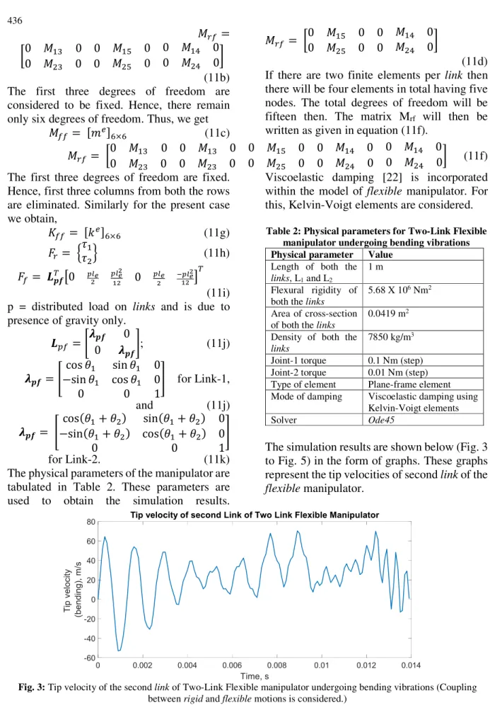
The simulation results are shown below (Fig. 3 to Fig. 5) in the form of graphs. These graphs represent the tip velocities of second link of the flexible manipulator.

Fig. 3: Tip velocity of the second link of Two-Link Flexible manipulator undergoing bending vibrations (Coupling between rigid and flexible motions is considered.)

0 0.002 0.004 0.006 0.008 0.01 0.012 0.014

Time, s

-60 -40 -20 0 20 40 60 80

T

ip

v

e

lo

ci

ty

(b

e

n

d

in

g

),

m

/s

Fig. 3 is obtained after solving equation (7a). The simulation stops after 0.018 second. This is because of the presence of coupling between

rigid and flexible motions in equation (7a). If

centrifugal and Coriolis terms are present then the simulation does not run. Step size of ‘0.1

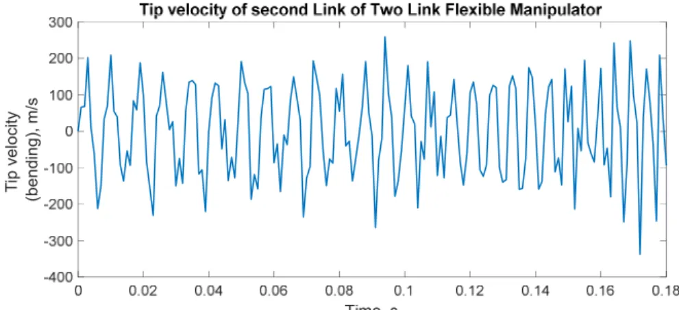
ms’ was used to obtain the above graph. When the coupling terms are reduced (say by a factor of 10000) the simulation runs for a longer duration. This can be observed from the following graphs.

Fig. 4: Tip velocity of the second link of Two-Link Flexible manipulator undergoing bending vibrations (Coupling between rigid and flexible motions is reduced by 10000.)

In Figure 4, it can be seen that tip velocity is high. The effect of centrifugal and Coriolis torques are considered while obtaining the

above results. The simulation stopped after 0.336 second. Step size of ‘1 ms’ was used to obtain the above graph.

Fig. 5: Tip velocity of the second link of Two-Link Flexible manipulator undergoing bending vibrations (Coupling between rigid and flexible motions is reduced by 10000; effect of gravity is considered.)

Figure 5 shows the tip velocity of second link

of the flexible manipulator when the effect of

gravity is considered along with the centrifugal and Coriolis torques. Step size of ‘1 ms’ was used. It is found that due to presence of gravity, the simulation stopped

after 0.207 second: earlier than the previous case. From the simulation results, it can be inferred that equation (7a) for the Two-link Flexible manipulator is highly non-linear.

4.1.2: Neglecting the effect of coupling between Rigidand Flexiblemotions The presence of coupling between the rigid

and flexible motions makes it difficult to solve

equation (7a). Hence, in this case coupling is removed and then the effect on simulation is observed. Before that, few changes are done in the dynamics

T

ip

ve

lo

ci

ty

(

b

e

n

d

in

g

),

m

/s

T

ip

ve

lo

ci

ty

(b

e

n

d

in

g

),

m

of the system. Analytically, the vibrating motion of an Euler-Bernoulli beam is given by following equation.

?:

-?D: + >_“<=@?

”

-?/” = {( , ) (12)

In above equation, w = deflection of beam, E = Young’s modulus of beam, I = area moment of inertia of beam, ρ = mass density of beam, A =

area of cross-section of beam and f(x,t) = external force acting on the beam. The analytical solution of equation (12) can be obtained using the approach of AMM [23]. Since approach of FEM is followed in this paper, equation (12) can be discretized to yield equation (8a). The load vector Ff is now

reformulated to contain two types of loads. First one is due to the distributed load described by equation (11i) and the second type of load is due to the excitation provided by the actuators placed at joints.

4.2 Calculation of excitation forces acting at the tips of the links

Fig. 6 (provided at the end) helps to understand the excitation forces acting at the tips of the

links. These forces are calculated as follows. { = •.

– = •.

8. (perpendicular to OA)

(13a)

{ = •:

—= •:

8: (perpendicular to AB)

(13b)

{ = •.

–— (perpendicular to OB) (13c)

Net force acting at B (perpendicular to AB), fbB = f22 + f21 cos(θ2-ϕ) (13d)

Net force acting at B (along AB), faB = f21

sin(θ2-ϕ) (13e)

Hence, load vector for the element containing the tip of the given link as one of its nodes can

be described as follows:

GM= Š‹Œ_0 •Žp: •Žp:.: 0 •Žp: + { ••Žp:.:` for Link-1, and (13f)

GM= Š‹Œ_0 •Žp: •Žp:.: 0 + {˜— •Žp: + {— ••Žp:.:` for

Link-2. (13g) The load vectors for remaining elements remain same as provided by equation (11i). Since, torsional vibrations are not considered here, hence the axes Z-Z1 and Z-Z2 (Fig. 1) will

always be parallel to each other. The load vector can be described in another way as follows:

GM= Š‹ŒX0 •tŽp: •tŽp:.: 0 •tŽp: ••tŽp:.: − I Z for Link-1, and (13h)

GM= Š‹ŒX0 •tŽp: •tŽp:.: 0 •tŽp: ••tŽp:.: − I − I Z for Link-2. (13i) It is to be noted that the load vectors described in equation (13f) to equation (13i) are only for the last elements of Link-1 and Link-2 respectively. Figure 7 shows the tip velocity of second link of the flexible manipulator when

coupling between rigid and flexible motions

are not considered.

Fig. 7: Tip velocity of the second link of Two-Link Flexible manipulator undergoing bending vibrations (Coupling between rigid and flexible motions is not considered; effect of gravity is not considered.).

In Figure 7, effect of gravity is not considered while the effect of centrifugal and Coriolis torques are taken into account. It can be observed that the simulation runs for a longer duration of time. After observing the simulation results from Fig. 3 to Fig. 7, it can

be concluded that the Two-Link Flexible manipulator is a highly non-linear system due to the presence of coupling between rigid and flexible motions, presence of gravity and

presence of centrifugal and Coriolis terms in the equation of motion (equation 7a).

T

ip

v

e

lo

c

it

y

(b

e

n

d

in

g

),

m

4.3 Results using combined bending-torsion vibrations

After obtaining results for bending vibrations, torsional effects are also included. Thus, the following results are for combined bending-torsional vibrations. For this, Space-frame elements are used. Damping is not considered while obtaining these results.

Equations- 13a to 13i describe the tip forces and tip load vectors. In case of coupled bending-torsion vibrations some additional forces will also act at the tips. Following equation describes the force acting at the tip of first flexible link, responsible for torsional

vibrations.

zy z|+ x H™} i z x{ $z|^ − 1, - =

{ š (2( + 2( ) (14)

Table 3: Physical parameters for Two-Link Flexible manipulator undergoing combined

bending-torsional vibrations Physical parameter Value Length of both the links,

L1 and L2

0.5 m Flexural rigidity of

Link-1 (E1I1y and E1I1z)

14.93 Nm2

Flexural rigidity of Link-2 (E2I2y and E2I2z)

1.017 Nm2

Area of cross-section of Link-1

4 cm x 4 mm Area of cross-section of

Link-2 5.17 cm x 1.5 mm

Density of both the links 7850 kg/m3

Modulus of rigidity of

both the links 8.08 x 10

11 _N/m2

Joint-1 torque Square wave of amplitude 0.05 Nm and time period 0.1s

Joint-2 torque Square wave of amplitude 0.01 Nm and time period 0.1s Type of finite element

used Space-frame element

Solver Ode45

This twisting torque acts perpendicular to plane: Y1-Z1, i.e. along X1 axis (refer to Fig. 6

and Fig. 1). This torque vector when seen from global frame (axes: X-Y-Z in Fig. 1) will have two rectangular components along X-axis and Y-axis. Besides that, gyroscopic couples will also act on the tips. The expressions for gyroscopic couple are given as follows.

[› xylx zl lx™ w} i z x{ $z|^ − 1, [d = œ• )6 ž 6 + Ÿ6 (15a)

The couple GC1 will act along Y1-axis; )6

represents the rate of twist of Link-1 about local X1-axis, Ÿ6 represents the rate of change

of slope of tip of Link-1 due to bending about Z1-axis and Jm1 is the mass moment of inertia

of Link-1.

[› xylx zl lx™ w} i z x{ $z|^ − 2, [d = œ• ž)6 − )6 cos ž 6 + Ÿ6 +

6 + Ÿ6 (15b) The couple GC2 will act along Y2-axis; )6

represents the rate of twist of Link-2 about local X2-axis, Ÿ6 represents the rate of change

of slope of tip of Link-2 due to bending about Z2-axis and Jm2 is the mass moment of inertia

of Link-2. The local force vectors for the elements containing tips of the links as one of

their nodes are given by equations- 15c and 15d provided at the end.

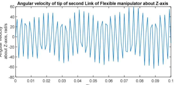
Fig. 8: Angular velocity of tip of second flexible link about Z-axis

A

n

g

u

la

r

v

e

lo

c

it

y

a

b

o

u

t

Z

-a

x

is

,

ra

d

Fig. 9: Linear velocity of tip of second flexible link along Z-axis

Fig. 10: Angular velocity of tip of second flexible link about Y-axis

Fig. 11: Linear velocity of tip of second flexible link along Y-axis

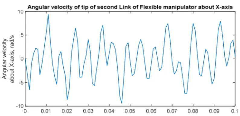
Fig. 12: Angular velocity of tip of second flexible link about X-axis

L

in

e

a

r

v

e

lo

c

it

y

a

lo

n

g

Z

-a

x

is

,

m

/s

A

n

g

u

la

r

v

e

lo

ci

ty

a

b

o

u

t

Y

-a

xi

s,

r

a

d

/s

L

in

e

a

r

ve

lo

ci

ty

a

lo

n

g

Y

-a

x

is,

m

A

n

g

u

la

r ve

lo

city

a

b

o

u

t X

-a

x

is, r

a

d

Fig. 13: Linear velocity of tip of second flexible link along X-axis The undamped tip responses of second flexible

link are shown in Fig. 8 to Fig. 13. From above

graphs, it can be observed that the angular velocity about Z-axis (Fig. 8) is the maximum while the linear velocity about Y-axis (Fig. 11) is the maximum.

4.4 Effect of vibrations on positional accuracy

Now, the effect of vibration of flexible links on

the positional accuracy of the end point of the second link (point B in Fig. 6) will be shown.

The physical parameters provided in Table 2 are taken for the simulation. The length of the position vector of point B is given by ‘OB’. It can be found out as follows:

¡¢ = £š—+ ¤— + ¥— (16)

XB, YB and ZB are the coordinates of point B

(Fig. 6) w.r.t. ground frame XYZ (Fig. 1 and Fig. 2). These coordinates are calculated using equation (2). Fig. 14 shows the variation of length of position vector OB for a Two-Link Rigid manipulator and a Two-Link Flexible manipulator undergoing both bending and torsional vibrations. It is to be noted that the

rigid manipulator operates in X-Y plane only.

Hence, its Z-coordinate remains zero throughout. But for the flexible manipulator,

due to presence of torsional vibrations, the

links show some deflections in Y-Z plane also.

Hence, the flexible manipulator undergoing

both bending and torsional vibrations, no longer remains planar.

Fig. 14: Comparison of length of position vectors of the tip of second Link for a Two-Link Rigid and Flexible manipulators (The flexible manipulator undergoes coupled bending and torsional undamped vibrations; BT means

Bending-Torsion). In Figure 14 and Figure 15, BT stands for

‘Bending-Torsion’. Figure 15 shows the three-dimensional plot of position of tip B (Fig. 6) of the flexible manipulator. When only bending

vibrations are present, the flexible manipulator

remains in X-Y plane, i.e., it can be said to be planar.

T

ip

ve

lo

city

a

lo

n

g

X

-a

x

is, m

/s

L

e

n

g

th

o

f

p

o

s

it

io

n

v

e

c

to

r

o

f

ti

p

,

Fig.15: 3D-plot showing the position of tip of second Flexible Link for undamped vibrations. In figure 15, the red coloured graph is for the

flexible manipulator undergoing coupled

bending-torsional (BT) vibrations while the blue coloured graph is for the flexible

manipulator undergoing only bending vibrations. It is clear from the figure that presence of torsional vibrations severely

deteriorates the positional accuracy of the tip B.

4.4.1 Frequency analysis of undamped vibrations of Flexible Links

Table 3 gives the natural frequencies of the Two-link Flexible manipulator for two finite elements (FEs) and ten finite elements (FEs). Table 4: Natural frequencies of Flexible Manipulator

S. No. Natural Frequency (using FEM)

2 FEs 10 FEs

1 1.6 2.05

2 2.1 2.07

3 5.7 6.99

4 7.1 7.00

5 27.5 19.9

6 35.3 20.5

7 56 39.6

8 71 42.6

9 1019 60.46

10 1497 67.3

11 1646.5 98.6

12 4229.4 112.9

13 - 132.07

14 - 153.79

15 - 175.52

16 - 184.78

17 - 245.2

18 - 248.3

19 - 302.87

20 - 336.13

21 - 391.53

22 - 425.97

23 - 449.47

24 - 462.91

25 - 508.78

26 - 587.4

27 - 592.88

28 - 651.24

29 - 705.69

30 - 779.52

Z

-co

o

rd

in

a

te

,

Above frequencies were matched using FFT analyses. Fig. 16 to Fig. 18 show the

FFT of the vibration of tip B of the flexible

manipulator undergoing coupled bending-torsional vibrations.

Fig. 16: FFT analysis of X-axis vibrations of tip B From Fig. 16, it is found that the dominant

frequencies are about: 40 Hz (near to 42.6 Hz in Table 4, column 3) and 70 Hz (near to 67.3 Hz in Table 4, column 3).

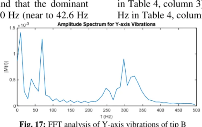
Fig. 17: FFT analysis of Y-axis vibrations of tip B From Fig. 17, it is found that the dominant

frequencies are about: 7 Hz (7 Hz in Table 4, column 3), 70 Hz (near to 67.3 Hz in Table 4, column 3) and 300 Hz (near to 302.87 Hz in Table 4, column 3). All these frequencies are present in Table 3. Besides that, other

identifiable frequencies are about: 40 Hz (near to 39.6 Hz in Table 4, column 3) and 250 Hz (near to 248.3 Hz in Table 4, column 3). There are very small peaks between 100 Hz to 200 Hz. All these frequencies can be identified to be present in Table 3.

Fig. 18: FFT analysis of Z-axis vibrations of tip B From Fig. 18, the dominant frequencies are

about: 35 Hz (near to 39.6 Hz in column 3 and 35.3 Hz in column 2 in Table 4), 56 Hz (near to 56 Hz in column 2 and 60.46 Hz in column 3 in Table 4) and 350 Hz (near to 336.13 Hz in column 3, Table 4). The accuracy of FFT analysis depends upon the sampling frequency and sample size. For the present case, the

sampling frequency is 1000 samples per second and sample size is 100.

5. VALIDATION OF MATHEMATICAL

MODEL

The validation of mathematical model is done with the results of [24]. The physical parameters are given in Table 5.

|M

(f

)|

|M

(f

)|

|M

(f

Table 5: Physical parameters (as used by Chiaming et. al.) for validation

Physical parameters Values Length of each link L1 = L2 = 1 m

Mass of each link m1 = m2 = 5 kg

Young’s modulus E1 = E2 = 2 X 1011 N/m2

Second moment of area I1 = I2 = 5 X 10-9 N/m2

Initial conditions θ1 = 0⁰; θ2 = 5⁰

Joint 1 torque 0 Nm

Joint 2 torque Half sine wave of amplitude 2 Nm and duration 1 second. The simulation results are shown in Fig. 19-21. To obtain these results, two finite elements are used during simulation, i.e., one finite element per link. The first two lowest frequencies of the flexible manipulator are found out to be: 2 Hz

and 12 Hz.

Fig. 19: Comparison of joint responses of Two-Link Flexible manipulator between present work and Chiaming’s work Figure 19 shows the joint responses of the

flexible manipulator. These are compared with

the results of Chiaming. It is found that the

joint responses found in present work are close

to the joint responses obtained by Chiaming.

Fig. 20: Tip displacement of Link-1 of the Flexible manipulator

Fig. 21: Tip displacement of Link-2 of the Flexible manipulator Figure 20 shows the tip displacement of

Link-1 along global Y-axis and Fig. 2Link-1 shows the tip displacement of Link-2 along global Y-axis. It is found that the forced response (between 0 to

1 second) of the tips match well with the results of Chiaming but the transient responses do not match. In the present work, the transients exhibit the frequency of 2 Hz while in the work

J

o

in

t

a

n

g

le

,

ra

d

D

isp

la

ce

m

e

n

t

o

f

ti

p

1

,

m

D

is

p

la

c

e

m

e

n

t

o

f

ti

p

2

,

of Chiaming, the transients exhibit the frequency of less than 2 Hz. It is notable that for the parameters of the flexible manipulator

given in Table 5, the lowest natural frequency is found out to be 2 Hz which is same as being exhibited by the graphs in Figure 20 and Figure 21.

6. CONCLUSIONS

In this paper, Lagrangian-finite element method is used to obtain the dynamic model of a Two-Link Flexible manipulator. Two types of finite elements are considered for discretization of the flexible links. These are:

‘space frame element’ and ‘plane frame element’. Coupling between rigid and flexible

degrees of freedom is considered and its effect on simulation is shown. It is found that this coupling makes the system highly non-linear and the solutions to the equations of motion do not converge. In order to obtain results, the equations of motion are modified suitably and discussed within the paper. The effect of non-linearity due to the presence of centrifugal, Coriolis and gravity terms are also shown in the paper. The novelty of the paper lies in inclusion of torsional vibrations of the links

along with the flexural vibrations. It is shown that due to the presence of torsional effect, the

flexible manipulator no longer remains planar.

The torsional vibrations severely deteriorate the positional accuracy of the manipulator.

REFERENCES

[1] Benosman and Vey, Control of flexible manipulators: A survey, Robotica, Vol 22,

pp. 533-534, 2004.

[2] S. K. Dwivedy, Peter Eberhard, Dynamic analysis of flexible manipulators, a review,

Mechanism and Machine Theory, pp. 749-777, 2006.

[3] Sunada and Dubowsky, The application of finite elements methods to the dynamic analysis of flexible spatial and co-planar linkage systems, Journal of Mechanical

Design,Vol 103,pp. 643-651, 1981.

[4] Dado and Soni, A generalized approach for forward and inverse dynamics of elastic manipulators, IEEE,pp. 359-364, 1986.

[5] Nagnathan and Soni, Non-linear flexibility studies for spatial manipulators, IEEE, pp.

373-378, 1986.

[6] Usoro, Nadira, Mahil, A Finite Element/ Lagrange approach to modelling lightweight flexible manipulators, Journal of Dynamic

Systems, Measurement and Control, Vol. 108,pp. 198-205, 1986.

[7] E. Bayo, A finite-element approach to control the end-point motion of a single-link flexible robot, Journal of Robotic Systems, Vol. 4,pp.

63-75, 1987.

[8] Simo and Vu-Quoc, The role of nonlinear theories in transient dynamic analysis of flexible structures, Journal of Sound and

Vibration, Vol. 4,pp. 63-75, 1987.

[9] Tzou and Wan, Distributed structural dynamics control of flexible manipulators-I, Structural dynamics and distributed viscoelastic actuator, Computers &

Structures, pp. 669-677, 1990.

[10] Chedmail, Aoustin and Chevallereau,

Modelling and control of flexible robots,

International Journal for Numerical Methods in Engineering, Vol. 32, pp. 1595-1619, 1991.

[11] Alberts, Xia, Chen, Dynamic analysis to evaluate viscoelastic passive damping augmentation for the space shuttle remote manipulator system, Journal of Dynamic

Systems, Measurement and Control, Vol. 114,pp. 468-475, 1992.

[12] Gaultier and Cleghorn, A spatially translating and rotating beam finite element for modelling flexible manipulators,

Mechanism and Machine Theory, Vol. 27, pp. 415-433, 1992.

[13] Hu and Ulsoy, Dynamic modeling of constrained flexible robot arms for controller design, Journal of Dynamic Systems,

Meadurement and Control, Vol. 116,pp. 56-65, 1994.

[14] Stylianou and Tabarrok, Finite element analysis of an axially moving beam, Part I: Time integration, Journal of Sound and

[15] Stylianou and Tabarrok, Finite element analysis of an axially moving beam, Part II: Stability analysis, Journal of Sound and

Vibration, Vol. 178,pp. 455-481, 1994.

[16] Theodore and Ghosal, Robust control of multilink flexible manipulators, Mechanism

and Machine Theory, Vol. 38, pp. 367-377, 2003.

[17] R. Fotouhi, Dynamic analysis of very flexible beams, Journal of Sound and Vibration, Vol.

305,pp. 521-533, 2007.

[18] Meghdari and Ghassempouri, Dynamics of Flexible Manipulators, Journal of

Engineering, Islamic Republic of Iran, Vol. 7, pp. 19-32, 1994.

[19] Theodore and Ghosal, Comparison of the assumed modes method and finite element models for flexible multilink manipulators,

The International Journal of Robotics Research, Vol. 14,1995.

[20] Chandrupatla and Belegundu, Introduction to Finite Elements in Engineering, New Delhi:

PHI Learning Private Limited, Third Edition.

[21] Natraj Mishra, S.P. Singh, B.C. Nakra,

Dynamic Modelling of Two Link Flexible Manipulator using Lagrangian Assumed Modes Method, Global Journal of

Multidisciplinary Studies, Vol.-4, Issue-12, pp. 93-105, 2015.

[22] D. R. Bland, The Theory of Linear Viscoelasticity, London: Pergamon Press,

1960.

[23] S. Rao, Mechanical Vibrations, Pearson,

Fourth Edition.

[24] Chiaming Yen, Glenn Y. Masada, Wei-Min Chan, Dynamic Analysis of a Two-link Flexible Manipulator System using Extended Bond Graphs, Journal of the Franklin

Institute, Vol. 330, No. 6,pp. pp. 1113-1134, 1993.

[25] W. Chen, Dynamic modeling of multi-link flexible robotic manipulators, Computers &

Structures, pp. 183-195, 2001.

Fig. 2: Dynamics modelling of Two-Link Flexible manipulator using two Space-frame finite elements.

\]& = J\ ] & _\

] &

\& ] \& ]N (8e)

\& ]=

⎣ ⎢ ⎢ ⎢ ⎢

⎡2§ƒ

0 0 0 0 0

0 156§

0 0 0

22w]§

0 0 156§

0

22w]§

0 0 0 0

2§v

0 0

0 0

22w]§

0

4w]§

0

0

22w]§

0 0 0

4w]§ ⎦

⎥ ⎥ ⎥ ⎥ ⎤

; θ1

θ2

w2(x2, t)

w1*

X1

X Y

X

Y Y2

Link 1

Link 2

Joint 1

Joint 2

Node 2

Node 3

Q_{6i - 4}

Q6i - 5

i (Node)

Node 1

Q_{6i - 3}

Q_{6i - 2} Q_{6i - 1}

\& ]= ⎣ ⎢ ⎢ ⎢ ⎢

⎡§₀ƒ

0 0 0 0 0 54§ 0 0 0

13w]§

0 0 54§

0

13w]§

0 0 0 0 §v 0 0 0 0

−13w]§

0

−3w]§

0

0

−13w]§

0 0 0

−3w]§ ⎦

⎥ ⎥ ⎥ ⎥ ⎤

\& ]=

⎣ ⎢ ⎢ ⎢ ⎢

⎡§₀ƒ

0 0 0 0 0 54§ 0 0 0

−13w]§

0 0 54§

0

−13w]§

0 0 0 0 §v 0 0 0 0

13w]§

0

−3w]§

0

0

13w]§

0 0 0

−3w]§ ⎦

⎥ ⎥ ⎥ ⎥ ⎤

\& ]=

⎣ ⎢ ⎢ ⎢ ⎢ ⎡2§ƒ 0 0 0 0 0 0 156§ 0 0 0

−22w]§

0 0 156§

0

−22w]§

0 0 0 0 2§v 0 0 0 0

−22w]§

0

4w]§

0

0

−22w]§

0 0 0

4w]§ ⎦

⎥ ⎥ ⎥ ⎥ ⎤

In above matrices, _{§ = § =}“_{v 9}pqp; _{§ƒ =}“_upqp; _{§v =}B_u« (8f) where, ρ = mass density of the element, and Jm = mass moment of inertia of the element.

{&_{= X0} •rqp •tqp ₀ ˆ•rqp: •tqp: ₀ •rqp •tqp ₀ •rqp: ˆ•tqp:_{Z (8g)}

where, py and pz are the distributed loads on the element along y- and z-directions respectively.

Gx $z|^ − 1, {&_{= X0} •rqp •tqp ₀ ˆ•rqp: •tqp: ₀ •rqp •tqp _{0 +}

- •rqp:+ [d ˆ•tqp:− I Z (15c)

Gx $z|^ − 2, {& _{= X0} •rqp •tqp ₀ ˆ•rqp: •tqp: ₀ •rqp •tqp ₀ •rqp:_{+ [d} ˆ•tqp:_{− I − I Z (15d)}

Fig. 6: Calculation of excitation forces at the ends of links O (Joint 1)

A (Joint 2) Link 1

B

θ

θ

Payload

φ

f

ANALIZA DINAMICĂ A MANIPULATORULUI FLEXIBIL CU DOUĂ LEGĂTURI

FOLOSIND FEM ÎN CURS DE ÎNDOIRE-TORSIUNE VIBRAȚII

Rezumat: În această lucrare, un manipulator flexibil cu două legături este analizat folosind o abordare

cu elemente finite ale cărei legături sunt în curs de îndoire combinatăși vibrații de torsiune. Modelul

matematic al manipulatorului flexibil se obține folosind dinamica lagrangian. Link-urile sunt

modelate ca grinzi Euler-Bernoulli și discretizate folosind "spațiu-cadru" și "plan-cadru" elemente.

Lucrarea prezentă tratează diverse efecte neliniare ar fi, cuplarea între grade rigide și flexibile de

libertate, efecte centrifuge și Coriolis și prezența gravitației. Modelul matematic este validat folosind

rezultatele disponibile în literatura de specialitate. Noutatea prezentei lucrări constă în includerea

efectelor torsionale și evidențiind astfel efectele acestora asupra preciziei poziționale a

manipulatorului flexibil.

Natraj MISHRA, Assistant Professor, School of Engineering, UPES Dehradun, India, Email: [email protected]