by Rahul A. Parsa and Stuart A. Klugman
AbSTRACT
Regression analysis is one of the most commonly used
statisti-cal methods. But in its basic form, ordinary least squares (OLS)
is not suitable for actuarial applications because the
relation-ships are often nonlinear and the probability distribution of the
dependent variable may be non-normal. One approach that has
been successful in overcoming these challenges is the
gener-alized linear model (GLM), which requires that the dependent
variable have a distribution from the exponential family. In this
paper, we present copula regression as an alternative to OLS
and GLM. The major advantage of a copula regression is that
there are no restrictions on the probability distributions that can
be used. In this paper, we will present the formulas and
algo-rithms necessary for conducting a copula regression analysis
using the normal copula. However, the ideas presented here can
be used with any copula function that can incorporate multiple
variables with varying degrees of association.
KEYwORdS
to the left, while models for casualty losses are usu-ally skewed to the right. Furthermore, there is no log-ical argument, other than mathematlog-ical simplicity, to support a linear relationship between the covariates and the mean of the response variable. Embrechts, McNeil, and Straumann (2002) show how the Pear-son correlation coefficient can be misleading when the underlying distributions are not normal. They ad-vise using copulas to model data that are not normal because such models capture a greater variety of re-lationships (essentially being nonparametric).
A significant advance was provided by the devel-opment of the generalized linear model (GLM). The standard reference is McCullagh and Nelder (1989). The generalization comes in two places. First, the distribution of Y must be a member of the exponen-tial family (which includes many commonly used distributions such as binomial, Poisson, negative bi-nomial, normal, gamma, inverse Gaussian, and log-normal, see pages 26-28 of McCullagh and Nelder). Second, the relationship between the mean of Y and the covariates is expressed as E(Y | X1 = x1, . . . , Xk = xk) = g–1(b
0 + b1x1 + ??? bkxk) where g(y) is called the link function. The conditional variance of Y is no longer constant but will depend on the conditional mean. The nature of the dependence depends on the choice of distribution for Y. Modern statistical soft-ware includes GLM analysis for specific combina-tions of distribucombina-tions and link funccombina-tions. Estimation is done by maximum likelihood. This model has been widely used in automobile pricing and there are numerous articles providing actuarial applications (Aitkin 1989, Mosley 2004).
The next step in generalizing this model is to re-move the restriction that the distribution of Y be from the exponential family. There is nothing inherent in the GLM that demands the use of the exponential family, although some of the calculations become more difficult and there is no convenient expression for the conditional variance. This generalization is briefly discussed by Klugman, Panjer, and Willmot (2008) and is further expanded in Venter (2007).
We are proposing an alternative approach to gen-eralizing the OLS regression model. We are not
1. Introduction
Regression analysis is one of the most widely used statistical methods, dating back to Francis Galton’s 1875 discovery of the regression slope (Stanton 2001). The key concept behind this methodology is identifying a relationship between a set of vari-ables. The premise is that a dependent or response variable, labeled Y, is assumed to be related in some functional form to several covariates (also referred to as explanatory or independent variables), labeled X1, X2, . . . , Xk. The response variable, Y, measures a random quantity of interest. Examples include the annual claims on an automobile insurance policy and the age at death of an insured life. The covariates, X1, X2, . . . , Xk, could be a set of characteristics of the insured. For example, in automobile insurance the variables might be age, gender, accident history, credit score, and so on. In life insurance the variables might be age, gender, smoking status, blood pres-sure, height, weight, and so on. If it is possible to express how the distribution of the response variable is related to the covariates, the result is often a reduc-tion in the uncertainty of insured events that depend on Y.
The basic OLS regression model presents a spe-cific model for the relationship. The distribution of Y given the covariates is assumed to be normal with a variance that is constant (that is, not related to the co-variates) and a mean that is related to the covariates as E(Y | X1 = x1, . . . , Xk = xk) = b0 + b1x1 + ??? bkxk. The equivalent (in this case) techniques of maximum likelihood and least-squares are used to estimate the unknown coefficients. The covariates can be con-sidered as random observations (in which case it is assumed the complete set of variables has a multi-variate normal distribution) or as fixed quantities, for example, where the levels are set in a designed experiment. A measure of the success of the model is the reduction in the variance of Y through the use of the covariates. Basic OLS regression is covered in most introductory statistics texts.
distribution functions, the resulting function is a le-gitimate multivariate distribution function. The key is that the copula creates the dependence structure independently of the marginal distributions. This concept of defining a multivariate dependence struc-ture (and hence copula) is based on Sklar’s theorem, which states:
Sklar’s Theorem (Sklar 1959): Let F be an n-dimensional joint cumulative distribution function for the random variables X1, X2, . . . , Xn with marginal distribution functions F1(x1), F2(x2), . . . , Fn(xn). Then there exists a Copula function, C, such that
FX
1,...,Xn(x1, . . . , xn) = C[F1(x1), . . . , Fn(xn)].
If the marginal distributions are continuous, then C is unique. If any distribution is discrete, then C is uniquely defined on the support of the joint distribution.
In the case of continuous distributions, the mul-tivariate dependence structure and marginal dis-tributions can be separated and the copula can be considered “independent” of the margins (Joe 1997, pp. 12-13). The copula thus allows arbitrary continu-ous marginal distributions to be combined and de-scribes their dependence structure.
There are several bivariate and multivariate copula distributions discussed in the literature. Hutchinson and Lai (1990), Nelson (1999), Joe (1997) and Klug-man, Panjer, and Willmot (2008) are excellent texts that discuss various properties of bivariate copula distributions. Joe (1997) also discusses the proper-ties of several multivariate copula distributions. Em-brechts, McNeil, and Straumann (2002) use copulas to show how the Pearson correlation coefficient can be misleading. Klugman and Parsa (1999), and Frees and Valdez (1998) use copulas in modeling insur-ance data. Others who have contributed to the copula literature are Genest and MacKay (1986) and Miller and Liu (2002).
While many copula functions have been identi-fied, we believe only two are useful for building a regression model with several covariates. One of the features of any useful regression model is that the claiming that it is superior to GLM or OLS, but
rather that it provides an alternative that has the pos-sibility of providing a better fit to observed data. Begin by assuming that all the variables (response and covariates) are random observations from some joint probability distribution. Because some of the variables are dependent (if there are no dependen-cies, then possessing the covariates provides no use-ful information about the response variable) a model with dependence must be used. A popular method for creating a multivariate model with dependence is the copula model. There are numerous papers with actuarial applications of copulas. A good introduc-tion is provided by Frees and Valdez (1998). In this paper, we will use the normal copula for the reasons described in Section 2.
This paper will develop copula regression as fol-lows. Section 2 introduces copula functions and the normal copula. Section 3 covers parameter es-timation and computation of the conditional mean. Section 4 concludes the paper with comprehensive examples.
2. Copulas
Copulas are useful for describing multivariate non-normal distributions. They describe the depen-dence structure between the variables. Marginal dis-tribution functions are used as inputs to the copula and these can be any set of disparate distributions. Thus, a copula is a realistic way of describing the multivariate distributions, as the analyst normally has a good idea about each marginal distribution and seldom has a good idea about the joint distribution of these variables.
A copula model can be constructed as follows. Begin with n random variables with distribution functions FX
1(x1), FX2(x2), . . . , FXn(xn). The joint
dis-tribution function is created by applying the copula function, C, as
FX
1,...,Xn(x1, . . . , xn) = C[FX1(x1), . . . , FXn(xn)].
results of maximum likelihood estimation will match those from OLS. Thus, like GLM, this method is a (different) generalization of the OLS model.
3. Parameter estimation
The normal (multivariate normal) copula function is defined as (Song 2000)
CR(u1, . . . , un) = G[F–1(u
1), . . . , F–1(un)], (3.1) where F(u) is the standard normal cumulative dis-tribution function and G is the multivariate normal cumulative distribution with zero means, unit vari-ances, and correlation matrix R. The matrix R has ones on the diagonal and the off diagonal elements are correlations. However, it is important to note that when the normal copula is used these are not the cor-relations of the modeled variables.
Thus, for arbitrary marginals, the distribution function induced by the normal copula is
F(x1, . . . , xn)
= G{F–1[F
1(x1)], . . . , F–1[Fn(xn)]}. (3.2)
If the marginal distributions are continuous then the density function is given by (Clemen and Reilly 1999, Nelson 1999)
f x( 1, . . . , xn)
= ⋅⋅⋅ − −
×
−
−
f x f x f xn n v R I v R
T
1 1 2 2
1
0
2
( ) ( ) ( )exp ( ) ..5,
(3.3)
where v is a vector with ith element vi = F–1[F
i(xi)] and I is the identity matrix. Note that if the correla-tions are all zero, then R is the identity matrix and the joint density is the product of the marginal densities and all the variables are independent.
This density function can then be used to deter-mine the likelihood function.
Since we will be estimating predicted values us-ing the conditional mean of Y given the independent variables, we will need the conditional distribution of xn given x1, . . . , xn–1. It is
degree of association (e.g., Spearman’s Rank Cor-relation) between the response variable and each co-variate need not be constant. We are aware of only two copula models that allow for this, the normal copula and its generalization, the t-copula (which is based on the multivariate Student’s t distribution. For example, see the list of copulas in Klugman, Panjer, and Willmot (2008, Chapter 7), where it can be seen that the other copulas do not allow for variations in the association measure. In a recent paper by Crane and Van Der Hoek (2008) they use arbitrary bivari-ate copulas for building regression models. Because their methods do not extend to multivariate situa-tions, their approach is not useful for most applica-tions. Also, they do not address the case of discrete variables, which are common in practice.
Computing predicted values of Y using copula re-gression is a three-step process.
1. Assume a model for the joint distribution of all the variables (response and covariates),
2. Estimate the parameters of the model (the param-eters for the selected marginal distributions and the parameters of the copula), and
3. Compute the predicted values of Y given a set of covariates by using the conditional mean of Y given the covariates.
In this paper, we assume a normal copula model for the joint distribution of the variables and maximum likelihood for parameter estimation. For the normal copula explicit formulas for the likelihood function and conditional distribution are available. The condi-tional mean will usually need to be obtained by nu-merical integration. Because this is a one-dimensional integration, there are well-established accurate algo-rithms for obtaining the answer. Thus, this ease of use is one of the reasons we have selected the normal copula. The methodology presented in this paper can be used with other multivariate copulas (such as t or elliptical), but they would require extensive numerical analysis.
use the estimates from the marginal distributions as starting values for the global maximization (which is optimal). We used the latter procedure for estimating the parameters. This was done numerically. One au-thor used the solver tool in Excel and the other auau-thor used SAS IML and the NLPTR optimization proce-dure (NLPFDD to compute the Hessian matrix).
When any of the marginal distributions are discrete, there is an additional problem. This is illustrated with an example. Let X take on the values 0, 1, and 2 with probabilities 0.3, 0.4, and 0.3 respectively. Let Y be the other marginal with a uniform (0,1) distribution. Consider the independence copula. Now consider the contribution to the likelihood function for the obser-vation x = 1 and y = 0.6. It is the product of the prob-ability function of X at 1 and the density function of Y at 0.6, which is 0.4(1) = 0.4. But now suppose the nor-mal copula is being used. This requires calculation of cumulative probabilities from the multivariate normal distribution (in order to obtain the discrete probabil-ity), a non-trivial task. In addition, if there are several discrete variables, the probabilities for higher dimen-sional cubes will be required.
In OLS and GLM regressions, distributions for the covariates are usually not specified. In a copula model these distributions must be specified. How-ever, there is an easy way to replicate this situa-tion—for the marginal models, use the empirical distribution. Thus, in many applications all of the covariates will be modeled as discrete variables. The same problem affects conditional distributions.
Our recommended solution is to replace each discrete distribution with a continuous distribution. The simplest choice is to use a kernel density with a uniform kernel and a small bandwidth. In particular, select the bandwidth so that it is less than half the distance separating the two closest discrete probabil-ity points.
The likelihood function requires the kernel density pdf and cdf at each data point. Let b be the band-width. For any observed value, let p(x) be the prob-ability function and P(x) be the distribution function of the discrete distribution. For writing the likelihood function, for an observation at x, the kernel density
f x x( n 1, . . . , xn−1)= f xn( )expn
− − − − − − − − − − 0 5 1 1 1 1 2 1 1 1
. {F [ ( )]F x r R v*} {F [
r R r F
n n T n
T n
nn( )]}xn
2 × − (1 −−1 )−/
1 1 2
r R rT
n (3.4)
where v* = (v1, . . . , vn–1) and R R r r n T = −1 1
where r is an n – 1 3 1 vector that is the right-most column of R with the last element removed.
In the regression context, Xn will be the response variable (Y). Thus, this is the density function of the response variable given the covariates. The expected value is the predicted value (the median could also be used) and the standard deviation is equivalent to the standard error in OLS regression. However, the standard deviation will not be constant as it is in OLS regression.
Maximum likelihood estimates are asymptotically normal with covariance matrix given by the inverse of Fisher’s information matrix (I(u)–1). To use this result,
we would have to calculate the second derivatives of the likelihood function and take their expected values. In this problem, it is difficult to calculate second deriv-atives and their expected values, so we instead use the observed information matrix (Klugman, Panjer, and Willmot 2008). Once again, this is a well-understood problem. Most commercially available numerical analysis software provides the Hessian matrix, which is used to estimate the asymptotic covariance matrix (inverse of the Hessian matrix) for the estimates. We present this for Example 1 in Section 4.
To simulate the 50 trivariate data points (see the Appendix for the simulated data), we used the meth-odology described in Clemen and Riley (1999). It uses the following process:
Let Fi(xi), i = 1,2,3 be specified along with the cor-relation matrix.
1. First generate a vector (u1, u2, u3) from a multivar-iate normal distribution with zero means and unit variances and the specified correlation matrix. 2. Calculate si = F(ui) for each of the three variables. 3. Calculate FX si
i
−1( ) , i = 1,2,3.
The resulting vector from step (3) will have the specified marginals and copula correlation structure (see Appendix 1 for one of the data sets).
We measured the error in estimation using
(Yi−Yˆ )i 2 and compared the results to OLS and
GLM (where appropriate). We chose OLS and GLM for comparison as they are the procedures commonly used in practice. Nowadays, GLM is commonly used whenever the distribution of the dependent variable is non-normal.
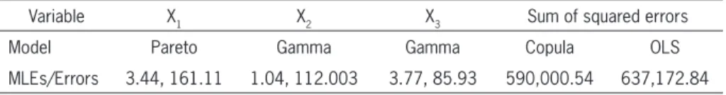
Example 1: The distributions of the three variables1
are: X1 ~ Pareto (a = 3, u = 100), X2 ~ Pareto (4, 300), X3 ~ Gamma (3,100) and X3 is the dependent variable. The parameters were estimated in two stages, using the method of maximum likelihood. In stage 1, only the data from the marginal distribution was used to estimate the parameters. In the second stage, the joint density was maximized using estimates from stage 1 as starting values. In this example, parameter esti-mates for X2 did not converge, so we approximated it using a gamma distribution. The copula regression model performed much better than OLS. The MLEs and errors are given in Table 1.
pdf is p(x)/(2b) and the cdf is P(x) – p(x)/2. Note that the value of b has no impact on the MLE.
For the conditional distribution, the only case that needs further study is when the response variable is discrete. The formula for the conditional density function (for continuous variables) can be written
f x w( n )= f x g F xn( ) [ ( ), ],n n n w
where w represents all the other variables, and g is defined by removing fn(xn) from (3.4). To obtain the discrete conditional probability it makes sense to in-tegrate the continuous conditional probability over the bandwidth:
p x wn p xn b
x b x b
n n
( )= ( )( )− −
+
∫
2 1×g P x[ ( )n n +p x t x( )(n − −n b) / ( ), ]2b w dt
= p x
∫
− + −b g P x p x z b w dz
n
n n
b b
( )
[ ( ) ( )( / . ), ] .
2 2 0 5
The second line follows from the transformation z = t – xn.
The integral must be evaluated numerically; the value of b has no impact on the result.
4. Examples
To illustrate our methodology, we present six ex-amples using simulated data. In all of the exex-amples, we have three variables—one dependent and two in-dependent and the sample size is 50 in all the cases. We use the same correlation matrix in all the exam-ples as given below.
R=
1 0 7 0 7 0 7 1 0 7 0 7 0 7 1
. .
. .
. .
1All variables are parameterized as in Klugman, Panjer and Willmot (2008).
Table 1. Parameter estimates and errors for Example 1
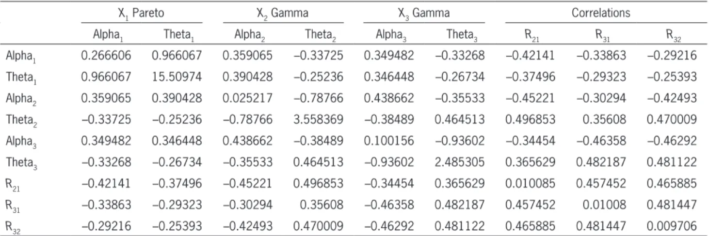
In Table 2 are the asymptotic standard deviations of the estimates and correlations among them (diag-onal terms are standard deviations and off-diag(diag-onal terms are correlations). The SAS IML procedure NLPFDD was used to calculate the Hessian matrix. It uses a finite difference approximation procedure to calculate the Hessian. We used the Hessian to cal-culate the observed information matrix (asymptotic variance matrix).
From this it is possible to construct confidence intervals. For example, the 95% confidence interval for alpha of the Pareto variable (X1) is given by 3.44 ± 1.96*0.266606.
The maximum likelihood estimate of the correla-tion matrix is given below.
ˆ . . ..
. .
. R=
1 0 711 0 699 0 711 1 0 713 0 699 0 713 1
As a reminder, while this is called a correlation matrix, it is merely the parameters of the normal cop-ula. These values do not represent the correlations of the marginal variables.
Example 2: Once again, the distributions of the three variables were: X1 ~ Pareto (a = 3, u = 100), X2 ~ Pareto (4, 300), X3 ~ Gamma (3,100) and X3 was the dependent variable. This time, instead of assuming a distribution for X1 and X2 and estimating the param-eters using MLE, we estimate the distributions
em-pirically. This is similar to OLS and GLM wherein we make no assumption on the distribution of the independent variables. Since the empirical distribu-tion is discrete, we approximated it by a continuous distribution and in particular we used the kernel den-sity with uniform kernel as previously described. We then took the limiting case of the uniform kernel as band width goes to zero, resulting in the following equations for the distribution and density functions (where x is one of the data points).
F x obs x
n
obs x n
( )= # ≤ −# =
2 and
f x n
( )=1
We also analyzed the data using a generalized linear model using the gamma distribution and log link. Once again, the copula regression model performed bet-ter than OLS and, much betbet-ter than GLM which per-formed very poorly. The results are given in Table 3.
The number of parameters in the various models is five for the copula model (two gamma parameters and three correlation coefficients, four for OLS (three re-gression parameters and the standard error), and four for GLM (three regression parameters and the gamma shape parameter). The large differences in the sums of squares are not likely due to the one parameter differ-ence. A more formal comparison might use the log-likelihood functions and an information criterion. Table 2. Asymptotic standard deviations
X1 Pareto X2 Gamma X3 Gamma Correlations
Alpha1 Theta1 Alpha2 Theta2 Alpha3 Theta3 R21 R31 R32
Alpha1 0.266606 0.966067 0.359065 –0.33725 0.349482 –0.33268 –0.42141 –0.33863 –0.29216 Theta1 0.966067 15.50974 0.390428 –0.25236 0.346448 –0.26734 –0.37496 –0.29323 –0.25393 Alpha2 0.359065 0.390428 0.025217 –0.78766 0.438662 –0.35533 –0.45221 –0.30294 –0.42493 Theta2 –0.33725 –0.25236 –0.78766 3.558369 –0.38489 0.464513 0.496853 0.35608 0.470009 Alpha3 0.349482 0.346448 0.438662 –0.38489 0.100156 –0.93602 –0.34454 –0.46358 –0.46292 Theta3 –0.33268 –0.26734 –0.35533 0.464513 –0.93602 2.485305 0.365629 0.482187 0.481122
R21 –0.42141 –0.37496 –0.45221 0.496853 –0.34454 0.365629 0.010085 0.457452 0.465885
R31 –0.33863 –0.29323 –0.30294 0.35608 –0.46358 0.482187 0.457452 0.01008 0.481447
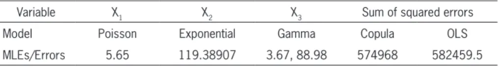
Example 3: The three variables are: X1 ~ Poisson (l = 5), X2 ~ Pareto (4, 300), X3 ~ Gamma (3,100) and X3 is the dependent variable. We estimated the parameters using the method of maximum likelihood in two stages as in Example 1. The distribution of X2 was approximated by an exponential distribution. Here again, the copula regression model did better than OLS. The results are given in Table 4.
Example 4: The situation is same as in Example 3 but the distributions of X1 and X2 were estimated empirically as in Example 2. Since X1 is discrete, its distribution was approximated by a continuous dis-tribution. Once again, we used the uniform kernel as in Example 2.
We also analyzed the data using GLM using gamma distribution and log link. The copula regres-sion model performed better than OLS and GLM.
Surprisingly, GLM performed the worst. The results are given in Table 5.
Example 5: The distribution of the three variables are X1 ~ Poisson (l = 5), X2 ~ Pareto (4, 300), X3 ~ Gamma (3,100), and X1 is the dependent variable. In this example, the dependent variable is discrete. The distribution of X2 was approximated by an exponen-tial distribution. In this example, the copula regres-sion model performed better than OLS. The results are given in Table 6.
Example 6: The situation is same as in Example 5 but the distributions of X2 and X3 are estimated em-pirically as in Example 2. The data were also ana-lyzed using GLM using the Poisson distribution and log link. The copula regression model performed the best and surprisingly, GLM performed the worst. The results are given in Table 7.
Table 3. Parameter estimates and errors for Example 2
Variable X1 X2 X3 Sum of squared errors Model Empirical Empirical Gamma Copula OLS GLM MLEs/Errors N/A N/A 4.0245, 81.0415 595,947.47 637,172.84 814,264.754
Table 4. Parameter estimates and errors for Example 3
Variable X1 X2 X3 Sum of squared errors Model Poisson Exponential Gamma Copula OLS MLEs/Errors 5.65 119.38907 3.67, 88.98 574968 582459.5
Table 5. Parameter estimates and errors for Example 4
Variable X1 X2 X3 Sum of squared errors Model Empirical Empirical Gamma Copula OLS GLM MLEs/Errors N/A N/A 3.96, 82.48 559,888.8 582,459.5 652,708.98
Table 6. Parameter estimates and errors for Example 5
Frees, E., and E. Valdez, “Understanding Relationships Using
Copulas,” North American Actuarial Journal 2, 1998, pp.
1–25.
Genest, C., and J. MacKay, “The Joy of Copulas: Bivariate
Dis-tributions with Uniform Marginals,” American Statistician
40, 1986, pp. 280–283.
Hutchinson, T. P., and C. D. Lai, Continuous Bivariate
Distri-butions, Emphasizing Applications, Adelaide: Rumsby Scien-tific Publishing, 1990.
Joe, H., Multivariate Models and Dependence Concepts,
Lon-don: Chapman and Hall, 1997.
Klugman, S., H. Panjer, and G. Willmot, Loss Models: From
Data to Decisions (3rd ed.), New York: Wiley, 2008. Klugman, S. and R. A. Parsa, “Fitting Bivariate Loss
Distribu-tions with Copulas,” Insurance: Mathematics and Economics
24, 1999, pp. 139–148.
McCullagh, P. and J. Nelder, Generalized Linear Models, New
York: Chapman and Hall, 1989.
Miller, D. J., and W. Liu, “On the Recovery of Joint
Distribu-tions from Limited Information,” Journal of Econometrics
107, 2002, pp. 259–274.
Mosley, R. C., “Estimating Claim Settlement Values Using
GLM,” Casualty Actuarial Society, Discussion Paper
Pro-gram, 2004,pp. 291–314.
Nelson, R. B., An Introduction to Copulas, New York: Springer,
1999.
Sklar, A., “Functions de Repartition a n dimensions et Leurs
Mar-ges,” Publications de l’Institut Statistisque de l’Universite de
Paris 8, 1959, pp. 229–231.
Song, P. X.-K., “Multivariate Dispersion Models Generated
from Gaussian Copula,” Scandinavian Journal of Statistics
27, 2000, pp. 305–320.
Stanton, J. M., “Galton, Pearson, and the Peas: A Brief History
of Linear Regression for Statistics Instructors,” Journal of
Statistics Education 9:3, 2001.
Venter, G., “Generalized Linear Models Beyond the Exponential Family with Loss Reserve Applications,” Casualty Actuarial
Society E-Forum, Summer 2007, http://www.casact.org/pubs/
forum/07sforum/07s-venter1.pdf.
Summary
In this paper, we have provided an alternative approach to generalizing OLS regression using a multivariate copula. When compared to GLM, the approach seems to be different rather than better or worse. Its strength lies in the ability to choose dis-tributions for dependent variables that are not mem-bers of the exponential family. Also, it allows the researcher to arbitrarily choose distributions for the marginals (GLM only requires specification of the distribution of the dependent variable). As skewed heavy-tailed distributions are common in insurance, this method provides a way to incorporate arbitrary distributions into regression models. Like GLM, this method allows nonlinear dependence to be modeled. Because correlation is not a useful measure of depen-dence in a non-normal world (Embrechts 2002), it is vital to describe the relationship between variables appropriately. In this regard, copula regression pro-vides a good alternative to OLS and GLM.
References
Aitkin, M., D. Anderson, B. Francis, and J. Hinde, Statistical
Modeling in GLIM, Oxford: Oxford Science Publications, 1989.
Clemen, R. T., and T. Reilly, “Correlations and Copulas for
De-cision and Risk Analysis,” Management Science 45, 1999, pp.
208–224.
Crane, G. J., and J. Van Der Hoek, “Conditional Expectation
Formulae for Copulas,” Australian and New Zealand Journal
of Statistics 50, 2008, pp. 53–67.
Embrechts, P., A. McNeil, and D. Straumann, “Correlation and Dependence in Risk Management: Properties and Pitfalls,”
Risk Management: Value at Risk and Beyond, ed. M. Demp-ster, pp. 176–223, New York: Cambridge University Press, 2002.
Table 7. Parameter estimates and errors for Example 6
Appendix 1
Data set used in Example 1
X1 - Pareto (3,100) X2 - Pareto (4,300) X3 - Gamma (3,100) 49.19615 168.9541 339.0285 59.79256 52.22341 239.234 69.32701 428.0111 507.1756 21.82025 26.6339 232.2198 80.69061 130.7855 391.3814 66.54305 168.3623 752.3682 75.11587 172.878 433.767 16.98576 52.90305 148.1844 29.07292 48.31109 159.9216 1.974758 9.093995 90.26908 50.54979 122.4136 161.8736 27.88491 258.5495 381.7534 8.246412 18.45999 206.3309 71.70904 82.3842 371.1022 13.82497 13.57812 185.7246 27.61229 16.27457 117.5737 37.53664 51.9417 168.9898 441.9211 265.2885 696.5949 50.09159 150.5714 550.9105 47.06166 171.4217 224.7604 3.752047 2.998249 191.9266 40.14482 69.7926 407.7342 1.809855 46.71836 215.6133 7.254417 42.41679 193.4215