Essays on antitrust issues

(1)

Essays on Antitrust Issues

Wonchul Hwang

A dissertation submitted to the faculty of the University of North Carolina at Chapel Hill in partial fulfillment of the requirements for the degree of Doctor of Philosophy in the Department of Economics.

Chapel Hill 2011

Approved by:

Gary Biglaiser, Advisor Peter Norman

(2)

ABSTRACT

WONCHUL HWANG: Essays on Antitrust Issues. (Under the direction of Gary Biglaiser.)

(3)

ACKNOWLEDGMENTS

I would like to thank the members of my dissertation committee including Peter Norman, Sergio Pareirras, Vijay Krishna and Brian McManus for the valuable comments on earlier drafts of this dissertation and their teaching theoretical and technical tools used in this dissertation. Most especially, I would like to thank my advisor Gary Biglaiser, for his excellent and considerate guidance. He was readily available and always provided me the exact direction throughout every step of my research. Of course, all errors herein are my own.

(4)

LIST OF FIGURES

2.1 Merger’s Profitability and Welfare Effect : Case 1 (S-S-R) . . . 14

2.2 Merger’s Profitability : Comparison . . . 16

2.3 Merger’s Welfare Effect : Comparison . . . 16

2.4 Merger’s Profitability and Welfare Effect : Case 2 . . . 18

2.5 Merger’s Profitability and Welfare Effect : Case 3 (No Efficiency Gain) . . . 20

2.6 Incentive of Merger - Rationalization . . . 25

2.7 Outsider’s Efficiency and Incentive of Merger . . . 26

2.8 Welfare Effect of Merger - Rationalization . . . 29

2.9 Profitability and Welfare Effect of Merger with Rationalization . . . 30

2.10 Welfare Effect of Profitable Merger - Synergy . . . 33

2.11 Synergy Effect and Profitability of Welfare-Increasing Merger . . . 34

2.12 Farrell-Shapiro’s Condition and Welfare-Increasing Merger . . . 41

2.13 Farrell-Shapiro’s Condition and Profitable Welfare-Increasing Merger . . . 41

2.14 Welfare-Increasing Merger Failing Farrell-Shapiro (10% Synergy) . . . 42

2.15 McAfee-Williams’ condition and Welfare-Increasing Merger . . . 44

2.16 McAfee-Williams’ condition and Profitable Welfare-Increasing Merger . . . 45

3.1 Example of Truth-telling Equilibrium . . . 93

4.1 EC Leniency Notice Cases . . . 97

4.2 Game Tree without Leniency Program . . . 103

4.3 Game Tree with Leniency Program . . . 108

A.1 Comparative Statics - Outsider’s Efficiency . . . 140

(8)

CHAPTER 1 Introduction

This document presents the three essays that form my dissertation in accordance with the Graduate School and Economics Department at UNC at Chapel Hill.

Chapter 2, titled “The Incentive of Horizontal Merger and Its Welfare Effect”, reexamines the result of Salant, Switzer, and Reynolds (1983) on horizontal merger’s private profitability, its welfare effect and price effect after I generalize their assumptions which include Cournot competition pre- and post-merger, identical constant marginal costs among firms and no entry-exit condition.

On one hand, collusion becomes easier post-merger if firms have constant and identical marginal costs. If such collusive effect exists, a merger becomes profitable but socially more injurious. On the other hand, cost saving from reallocation or synergies can make a merger profitable even under Cournot competition pre- and post-merger. A merger gets more prof-itable as insiders are more asymmetric, and outsiders are “less” efficient, while its welfare effect improves as insiders are smaller or more asymmetric, and outsiders are “more” efficient. Synergy-creating mergers are not always profitable or welfare-increasing. Consumer surplus (CS) increasing mergers are profitable, and CS-decreasing merger improves another profitable CS-decreasing merger’s profitability. Entry-inducing mergers are not always unprofitable while exit-inducing mergers are always profitable. Entry reduces a merger’s price effect or may even change the direction of it.

(9)

collusion agreement and its sustainability when each firm’s discount factor is private infor-mation. In order to analyze this issue, I construct a model where firms may have different discount rates and each firm does not know the other firms’ discount rate, and also build up an equivalent counterfactual model with perfect information. Then, I solve the model by using Bayesian Nash equilibrium or perfect Bayesian equilibrium concept and compare the features of equilibrium outcome with those under counterfactual model.

Under the private information, cartel could be agreed on even when each firm’s incentive constraint for cartel sustainability is not satisfied, and hence cartel agreement contains the possibility that cartel members produce more than cartel output from the beginning. If firms are allowed to agree on the payoff less than monopoly profit, there might exist a continuum of collusion equilibria where firms choose payoff below the monopoly payoff at the beginning. But the output in the first period plays the role of signaling that reveals each firm’s discount rate, so if both firms abide by the agreed output, perfect cartel output is produced from period 2 and on. When firms are allowed to agree on the uneven split of monopoly profit after communicating each other’s discount factor, truth-telling equilibrium does not exist under money transfer and may or may not exist depending on parameter values under output quota. Chapter 4, titled “Antitrust Policy Issues for Effective Cartel Deterrence”, deals with two antitrust policy issues : leniency program and crackdown policy. To examine the effectiveness of leniency program, I introduce cartel duration model and explain why self-reports are mostly made from “dying cartels” and applied simultaneously by multiple cartel members. These facts are the outcome path of stationary Markov perfect equilibrium in this model and the increase in the number of discovered cartels does not necessarily imply that the introduced leniency program is effective. Optimal law enforcement with leniency program, full exemption to deviator with no reduction to simultaneous leniency applicants, would increase deterrence to cartel if fines are sufficiently high or firm’s strategy against deviation is severe enough.

(10)

CHAPTER 2 The Incentive of Horizontal Merger and Its Welfare Effect

2.1 Introduction

Since Stigler (1950) pointed out “free rider’s problem” in horizontal merger meaning that firms who do not participate in a merger may get greater benefit than the constituent firms, the incentive of horizontal merger has been an important research topic in oligopoly market theory. Salant, Switzer, and Reynolds (1983) (“S-S-R” henceforth) provided one landmark paper on this issue. Employing a symmetric Cournot model with linear demand and identical constant marginal cost, S-S-R derived two surprising results on private profitability and social desirability of merger: (1) an exogenous merger may reduce the joint profits of the firms that are assumed to merge, and (2) a merger that provides efficiency gains may be socially beneficial even if it is privately injurious to the merging parties. On the first result, which took the name “The Merger Paradox”, they showed that it is sufficient for a merger to be unprofitable that less than 80% of the firms merge if there is no efficiency gains from the merger.

(11)

To start with, I consider the possibility that firms are engaging in tacit collusion post-merger. This extension shows that tacit collusion becomes easier after merger under the S-S-R model. If such collusive effect exists, the merger becomes profitable whereas it hurts consumers and worsens social welfare.

Another extension of the S-S-R model is to generalize the cost function. As Perry and Porter (1985) pointed out, mergers are not well-defined conceptually in the S-S-R model be-cause the merged entity does not differ from the others in their setting. In order to fix this shortcoming of the S-S-R model, I adopt and slightly modify the cost function that Perry and Porter (1985) proposed. This adjustment of the cost function enables me to capture the cost savings not only from reallocation among the facilities of constituent firms but also from synergies that a merger may create. In contrast, I maintain Cournot assumption of the S-S-R in this exercise because a merger does not necessarily reduce competition under this setting. The linear property of demand and marginal cost allows me to perform the direct analysis on the incentive of merger and its welfare effect. This model shows that a merger without synergies can be both privately profitable and socially desirable only when merging parties have quite different efficiency levels and outsider is sufficiently efficient. While the synergy effect improves both merger’s profitability and desirability, a merger with big synergies does not always bring higher welfare or consumer surplus. This extension also shows that a CS-increasing merger is always profitable. On the other hand, CS-decreasing merger may trigger another CS-decreasing merger, which can become profitable after the former CS-decreasing merger takes place.

Finally, I consider an environment where costless entry and exit is possible. Not surpris-ingly, entry (exit) may occur in a merger that would have been CS-decreasing (CS-increasing) under no entry-and-exit condition. Firms are less likely to merge under free entry condition, because entry harms merger’s profitability. But entry-inducing mergers are not always un-profitable whereas exit-inducing mergers are always un-profitable. The presence of entry or exit reduces a merger’s impact on price and may even change the direction of price effect.

(12)

Table 2.1: Key Feature of Each Model

Marginal Cost Competition Behavior Entry-exit Condition Section 2.3 identical + constant Cournot/collusion no entry-exit

Section 2.4 asymmetric + increasing Cournot no entry-exit

Section 2.5.1 identical + constant Cournot/collusion free entry-exit Section 2.5.2 asymmetric + increasing Cournot free entry-exit

effect of merger in this environment in Section 2.3. In Section 2.4, I construct the asymmetric increasing marginal cost model and perform the analysis on the incentive and welfare effect of merger in this setting. Section 2.5 extends these models in a direction where free entry or exit is allowed after merger. Concluding remarks are following in Section 2.6.

2.2 Literature Review

After S-S-R’s research, there have been many attempts to check the robustness of their results in various directions. Some researchers resolve the paradox by relaxing the assumption of linear demand [Cheung (1992), Fauli-Oller (1997), Hennessy (2000)], and others find the incentive of merger from product differentiation [Deneckere and Davidson (1985)], or earning and strengthening the position of Stackelberg leader [Perry and Porter (1985), Mallela and Nahata (1989)].

(13)

may hold in strategies other than trigger strategy.

When this paper deals with the collusive effect, it follows the “Folk Theorem” approach based on an infinitely repeated game setting. [Friedman (1971), Abreu (1986), Fudenberg and Maskin (1986) and etc.] In this approach, collusion is understood as a subgame perfect equilibrium in the repeated game. In more detail, firms interacting repeatedly may be able to maintain higher prices by agreeing that any deviation from the collusive path would trigger some retaliation. For the agreement to be sustainable, such retaliation must be sufficiently likely and costly to outweigh the short-term benefits from “cheating” on the collusive path. This paper illustrates that collusive effect may exist under the various retaliation strategies.

Another approach closely related to this research is to modify the S-S-R’s cost function. One attempt along this line is to use asymmetric but “constant” marginal cost functions across firms. Using this cost function and the linear demand, Fauli-Oller (2002) found that a merger can only be profitable if it involves firms that are asymmetric enough. This research confirms Fauli-Oller’s point that cost asymmetry is an important source of merger’s profitability, but it also shows that the degree of asymmetry necessary for a merger to be profitable depends on the outsider’s size or efficiency if asymmetric “increasing” marginal cost functions are assumed.

(14)

the scope of merger analysis. In particular, I can check the profitability, welfare effect and price effect of a merger with synergies.

This research is also closely related to the literatures on the welfare implications of merg-ers. Assuming Cournot competition pre- and post-merger as in the S-S-R model, Farrell and Shapiro (1990) provided the necessary and sufficient condition that a merger improves con-sumer surplus (Proposition 1), and the sufficient condition that a profitable CS-decreasing merger increases aggregate welfare (Proposition 5). As a special case where firms have asym-metric constant marginal costs, Froeb and Werden (1998) derives the condition on marginal cost reduction that restores the pre-merger price. The welfare analysis in this paper is another exercise of the Farrell-Shapiro model where demand is linear and cost function is linear or quadratic. Under these functional forms, I can derive a more specific and exact condition for welfare-increasing merger than Farrell-Shapiro’s Proposition 5. In addition, combining the welfare analysis of merger with the profitability analysis, I can get the properties of a merger that is privately profitable and socially desirable. In contrast, their Proposition 1 plays an essential role in my paper when I look at the profitability and welfare effect of a CS-increasing merger.

McAfee and Williams (1992), on the other hand, examined the welfare implications of horizontal mergers using linear demand and quadratic cost function with Cournot competition pre- and post-merger. They suggested a necessary condition for a merger to increase welfare, and showed that a merger reduces welfare if it creates a new largest firm or increases the size of the largest firm under moderately elastic demand. The asymmetric increasing marginal cost model has some common features with the McAfee-Williams model because both models assume linear demand and quadratic cost function. But this paper extends their research in that I include merger’s profitability and synergy effect into the scope of merger analysis. In particular, this paper demonstrates that their elasticity condition - the prerequisite to apply the McAfee-Williams’ condition - is too binding because profitable mergers fail to satisfy this condition.

(15)

Froeb (1998) showed that significant mergers are normally unprofitable or not so profitable to induce entry. Their result depends on two critical assumptions: the symmetry of cost function and no synergies. I illustrate that if these assumptions are relaxed, Cournot mergers can induce entry or even exit. Based on Bertrand setting, Cabral (2003) showed that cost efficiencies decreases the likelihood of entry, and thus benefit consumers less than under no entry condition. I confirm this result under Cournot setting and add the potential possibility that a marginal incumbent may exit post-merger under strong synergies. I also detail the price effect of entry-inducing or exit-inducing mergers.

Davidson and Muhkerjee (2007), on the other hand, demonstrated that any merger is profitable for any degree of cost synergy with free entry. Their result critically relies on the identical constant marginal cost function. This research shows that mergers creating synergies can be unprofitable even under no entry condition if the assumption on cost function is relaxed. Spector (2003) studied the price effect of a merger under free entry condition, and showed that any profitable Cournot merger failing to generate synergies raise price even if entry is possible. His result is an extension of Farrell-Shapiro’s Proposition 2 which proves the same argument under no entry condition. This research, in contrast, shows that if entry condition is relaxed when there is relatively “small” degree of synergies in that the merger with that amount of synergies would increase price under no entry condition, the merger’s price effect becomes not decisive.

2.3 Identical Constant Marginal Cost Model

(16)

2.3.1 Model

The model of this section considers an exogenous merger as in the S-S-R model, but the repeated game is constructed in order to see that the remaining firms makes collusion decision post-merger unlike the S-S-R model.

Demand and Supply : I assume linear demand and constant marginal cost. Specifically, demand curve is normalized as P = 1−Q and marginal cost as M C = 0.1 The demand and marginal cost do not change in every period t∈ {0,1,2,· · · }. There are N identical firms in the industry at period 0 that produce homogenous goods. Each firm discounts future profit at δ∈(0,1), which is the same and common knowledge across firms. Entry or exit does not take place in this economy.

Game Structure: Merger is one-time exogenous event under this model in the sense that all the remaining firms post-merger believe that there is no more merger. The timing of the game is as follows.

1. Firms compete`a la Cournot pre-merger at period 0.

2. (M + 1) firms merge at the end of period 0, whereM ∈ {0,1,· · · , N −1}.

3. Remaining firms make a collusion decision at the beginning of period 1.

4. Each firm chooses its output in every periodt≥1.

Each firm earns ₍_N₊₁₎1 2 at period 0 since the industry compete`a la Cournot. M is exogenous and represents the size of merger: no merger if M = 0; merger to monopoly if M = N −1. As in the S-S-R model, merger does not affect the marginal cost of merging firms. Efficiency gains take the form of saved fixed cost, F, if exists, which is assumed to be the same across all firms in the industry.

Stage Game Payoff Post-Merger : (N −M) firms remain in the industry post-merger and interact infinitely from period 1 and on. In each period post-merger, every firm would

1

(17)

get ₄₍_N1₋_M₎ under perfect collusion with symmetric payoff, ₍_N₋_M1₊₁₎2 under Cournot-Nash equilibrium. If a firm deviates with best response output when all other firms produce perfect collusive output (P

j6=iqcj = 2(NN−M−M−1)), its stage payoff would be

N−M+1 4(N−M)

2 .

2.3.2 The Effect of Merger on Firm’s Competitive Behavior

The merged entity is identical to the other remaining firms under this model. Let me denote the number of firms post-merger by L= (N −M) in this subsection, which may take a value from 1 toN. Then, the discounted payoff of each firm from perfect collusion is given by πC(L, δ) = ₄_L₍₁₋1 _δ₎ if L firms split monopoly profit evenly post-merger. In contrast, each firm’s discounted payoff becomesπD(L, δ) = L₄+1_L 2+r(δ, L) when it deviates and selects best deviation output. Here, r(δ, L) represents the discounted continuation payoff achieved under subgame perfect equilibrium in the punishment phase. It depends on firms’ strategy after unilateral defection. For example, r(δ, L) is ₍₁₋_δ₎₍δ_L₊₁₎2 in Nash reversion strategy [Friedman (1971)]. Then, collusion can be supported as subgame perfect equilibrium if and only if

πC(L, δ) ≥ πD(L, δ)

⇔ δ≥

L−1 L+ 1

2 +

4L L+ 1

2

(1−δ)∗r(δ, L) (2.1)

Letδ∗be the threshold discount rate such thatπC(L, δ∗) =πD(L, δ∗). By solving this equation, I can define δ∗ as a function of the number of firms (δ∗ =f(L)). If πC(L, δ) > πD(L, δ) for all δ ∈ (0,1), then f(L) ≡ 0, which means that collusion is agreed for any discount rate. If πC(L, δ) < πD(L, δ) for all δ ∈ (0,1), then f(L) ≡ 1, which means that collusion is never agreed. I assume that firms compete`a la Cournot ifδ≤δ∗ and collude with monopoly output if δ > δ∗. So I do not allow partial collusion if monopoly output cannot be supported as subgame perfect equilibrium outcome.

(18)

under these strategies as the number of firms decreases in the identical constant marginal cost setting. Given this result, I can assume that the threshold discount rate is strictly increasing in the number of firms (f0(L)>0).

2.3.3 Merger’s Profitability and Its Welfare Effect

Merger analysis of the identical constant marginal cost model also follows the S-S-R’s framework. But I now consider the possibility that a merger changes firms’ competitive be-havior, so I need to analyze a merger’s profitability and its welfare effect in all possible cases.

Framework of Merger Analysis

I will introduce some notations similar to the S-S-R for profitability analysis of merger. Πpre(N, M) denotes insiders’ pre-merger joint profits each period when the insiders consist of M+ 1 firms in an industry with N firms. Πpost(N, M) represents each period’s profits of the merged firm if the merger takes place amongM+ 1 constituent firms. The incentive of merger function, denoted by g(N, M), is defined as the increase in joint profits each period when a merger takes place amongM+ 1 insiders. So, by definition,

g(N, M) = Πpost(N, M)−Πpre(N, M)

Then if each firm’s per-period profit is given by Π(x) in an x-firm equilibrium, I get

Πpre(N, M) = (M+ 1)∗Π(N) Πpost(N, M) = Π(N −M),

sog(N, M) comes to

g(N, M) = Π(N −M)−(M + 1)∗Π(N) (2.2)

Given the assumptions on demand, marginal cost and firms’ competitive behavior, Π(x) = ₄1_x ifδ > f(x) while Π(x) = ₍_x₊₁₎1 2 ifδ ≤f(x).

(19)

welfare analysis of merger. S(N, M) is defined as per-period increase in total surplus when M+ 1 firms merge in an industry with N firms.

S(N, M) =T S(N, M)−T S(N) (2.3)

Here,T S(N, M) andT S(N) represent post-merger total surplus and pre-merger total surplus in each period, respectively. So, each term is defined by

T S(N, M) = CS(N, M) + (N−M)∗Π(N−M) T S(N) = CS(N) +N ∗Π(N),

whereCS(N, M) andCS(N) represent post-merger and pre-merger consumer surplus in each period, respectively.

In terms of firms’ competitive behavior post-merger, there are 3 possible cases depending on the number of firms before merger (N), the size of merger (M) and firms’ discount rate (δ); (Case 1) firms compete Cournot post-merger for everyM 6=N−1, (Case 2) firms collude post-merger for everyM 6= 0, and (Case 3) firms compete Cournot post-merger if merger size is less than threshold size (M < M∗) whereas they collude post-merger if merger size is equal to or larger than threshold size (M ≥M∗). In fact, (Case 2) is a special case of (Case 3) such that M∗ = 1. For example, suppose N = 10 and Nash reversion strategy is used against the unilateral defection. (Case 1) is applied for δ ≤ 9

17, (Case 2) for 25

34 < δ ≤ 121

161, and (Case 3)

for ₁₇9 < δ≤ 25

34. In (Case 3), M

∗ _{depends on the value of}_δ_.2

Even though I consider the infinitely repeated game situation,g(N, M) exactly reflects the private profitability of a merger to M+ 1 insiders because g(₁₋N,M_δ ) will be insiders’ increase in discounted profit from the merger, which is proportional to g(N, M). Then, it is enough to proceed the analysis withg(N, M). The same holds forS(N, M) in welfare analysis of merger.

Case 1. (S-S-R Model) : δ ≤f(2)

2_If_{δ >} 121

161 under our setting, firms are expected to collude pre-merger contrary to the assumption in this

(20)

This case happens when firms’ common discount factor is lower than threshold discount rate under duopoly (δ ≤f(2)). Since firms compete`a la Cournot pre- and post-merger under any size of merger except the one to monopoly, this is the case where all the results of the S-S-R model can be applicable.

Incentive of Merger: g1(N, M), the incentive of merger function in (Case 1), yields

g1(N, M) =

1

(N −M+ 1)2 −

M + 1

(N + 1)2 (2.4)

To compare with other cases, the results of S-S-R are summarized3:

Claim 1. [S-S-R] (a) A merger to form monopoly is profitable.

(b) For anyN, it is sufficient for a merger to be unprofitable that less than 80% of the firms merge.

A merger in (Case 1) is profitable if the concentration ratio of the merger α = M_N+1 is greater than the threshold concentration ratio ˆα(N) ≡ Mˆ+1

N ∈ [0.8,1). Put differently, every

merger combining ˆM+ 1 firms or more is profitable in (Case 1). I will call ˆM as the threshold merger size under the S-S-R.

Welfare Effect of Merger: S1(N, M), the welfare effect function in (Case 1), becomes4

S1(N, M) =

N−M (N −M + 1)−

N N + 1−

1 2

N−M N −M + 1

2 +1

2

N N + 1

2

(2.5)

Using this function, we can get the following result.

Claim 2. [S-S-R] (a) Every merger decreases welfare. (S1(N, M)<0 for all M 6= 0)

(b) Welfare decreases at a slower rate than the incentive of merger does

around M = 0.

∂g1(N,0)

∂M ≥

∂S1(N,0)

∂M

A merger in the S-S-R model decreases welfare because it does not bring any cost saving with increasing the remaining firms’ market power. But part (b) of this Claim implies that

3

Refer to Salant, Switzer, and Reynolds (1983) p.191∼p.195 for Claim 1 and Claim 2.

4

(21)

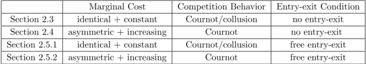
Figure 2.1: Merger’s Profitability and Welfare Effect : Case 1 (S-S-R)

social loss is smaller than private loss when the size of merger is small enough. This is because outsider’s profit gain outweighs consumers’ loss when a merger is sufficiently small.

Existence of Efficiency Gains: Efficiency gains turns the incentive of merger function into ˆg1(N, M) =g1(N, M) +M∗F. So, a merger that creates efficiency gains from elimination

of fixed cost duplication may still cause losses depending on the parameter values F and M. Social gain from a merger, on the other hand, becomes ˆS1(N, M) =S1(N, M) +M∗F. Since

∂g1(N,0)

∂M <0,

∂S1(N,0)

∂M <0, and

∂g1(N,0)

∂M

≥

∂S1(N,0)

∂M

for all N ≥2,it is possible to selectF so that ˆS1(N, M)>0>gˆ1(N, M) for someM.5Figure 2.1, which is quoted from Salant, Switzer,

5

(22)

and Reynolds (1983) (Figure 4. in pp.196), illustrates that a merger is privately unprofitable but socially desirable when the size of a merger (M) is less than k.

Case 2. f(N −1)< δ≤f(N)

This case happens when firms’ common discount factor is lower than threshold discount rate pre-merger, but becomes higher post-merger even under 2-firm merger (f(N−1)< δ≤f(N)). So any size of merger turns firms’ behavior into collusion in this case.

Incentive of Merger: g2(N, M), the incentive of merger function in (Case 2), yields

g2(N, M) =

     1 4(N−M)−

M+1

(N+1)2 if M >0

0 if M = 0

(2.6)

Since lim

M→0+

∂g2(N,M)

∂M <0 andg2(N, M) is convex,

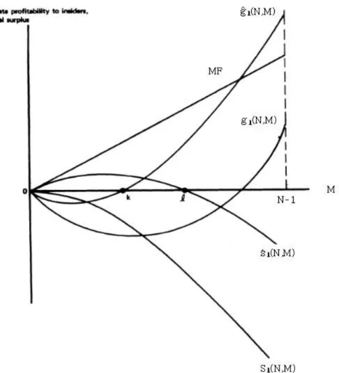
6 _{I can obtain the following results:}

Claim 3. (a) Every merger is profitable except M = N−1₂ while a merger is just break-even if

M = N₂−1 (g2(N, M)>0 for allM 6= N₂−1, andg2(N,N₂−1) = 0).

(b) A merger to form monopoly is strictly more profitable than a merger between

two firms. (g2(N, N −1)> g2(N,1) for allN >3)

The proof of every result in this paper is provided in the appendix. Claim 3 (a) shows that any size of merger is at least break-even to the insiders and strictly profitable if M 6= N₂−1. So, the incentive of a merger dramatically increases when the merger is expected to change firms’ competitive behavior from Cournot competition to collusion. Claim 3 (b) implies that a merger to monopoly is most profitable because g2(N, M) is convex andg2(N,N₂−1) = 0. Welfare Effect of Merger: The equilibrium price and quantity under Cournot compe-tition withN firms are given by P(N) = _N₊₁1 , Q(N) = _NN₊₁. So, consumer surplus amounts to CS2(N) = 1₂

N N+1

2

, and total profit of the industry is N ∗Π2(N) = ₍_NN₊₁₎2. Hence, T S2(N) = 1₂

N N+1

2

+₍_NN₊₁₎2. Since (N−M) firms collude post-merger in this case, the equi-librium price and quantity are given by P(N−M) = 1₂, Q(N−M) = 1₂. So, the post-merger

6

lim

M→0+

∂g2(N,M)

∂M = 1 4N2−

1

(N+1)2 <0 and

∂2g2

∂M2 =

(23)

Figure 2.2: Merger’s Profitability : Comparison

(24)

total surplus, T S2(N, M), comes toT S2(N, M) =CS2(N, M) + (N−M)∗Π2(N −M) = 3₈.

Hence,S2(N, M), the welfare effect function in (Case 2), yields

S2(N, M) =

  

 

0 if M = 0

4−(N+1)2

8(N+1)2 if M 6= 0

(2.7)

It is easy to see that S2(N, M) =

4−(N+1)2

8(N+1)2 < 0 for all N ≥ 2. So every size of merger causes social loss, and the amount of welfare loss does not depend on the size of merger. This is because the remaining firms collude for every M in this case. Comparing the incentive of merger and its welfare effect between (Case 1) and (Case 2), I can obtain the following result:

Corollary 1. Given the number of firms and the size of a merger not forming monopoly

(N, M),

(a) a merger in (Case 2) is more profitable than one in (Case 1) (g1(N, M)< g2(N, M));

(b) a merger in (Case 2) is socially more injurious than one in (Case 1)(S1(N, M)> S2(N, M)).

As expected, the private incentive to merge becomes higher and social welfare gets worse if Cournot competition turns to collusion after merger compared with the case that firms compete Cournot pre- and post-merger.

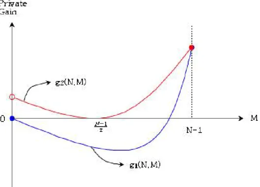
Existence of Efficiency Gains : If each firm has a fixed cost, the incentive of merger function comes to ˆg2(N, M) = g2(N, M) +M ∗ F. So every size of merger is profitable

because g2(N, M) ≥ 0 and M ∗ F > 0 for all M > 0. The welfare effect function turns

to ˆS2(N, M) = S2(N, M) + M ∗F. Note that ˆS2(N, M) and ˆg2(N, M) are largest when M = (N −1). So every size of merger is socially injurious if F ≤ ₈₍_N(N₋₁₎₍+1)_N2−4₊₁₎2, whereas a merger to monopoly is socially most desirable ifF > ₈₍_N(N₋₁₎₍+1)_N2−4₊₁₎2.

Case 3. f(N −M∗)< δ≤f(N −M∗+ 1) for some M∗ ≥2

(25)

(26)

Incentive of Merger : Without loss, suppose 2 ≤ M∗ ≤ N −2.7 For M < M∗, the post-merger competition is still Cournot. So, the gains of merging firms areg1(N, M) in this

area. For M ≥ M∗, firms collude post-merger. So, in this area, the gains of merging firms becomesg2(N, M). Hence, g3(N, M),the incentive of merger function in (Case 3), comes to

g3(N, M) =

  

 

g1(N, M) if M < M∗ g2(N, M) if M ≥M∗

(2.8)

Note thatg3(N, M) is convex both in [0, M∗) and [M∗, N−1]. A merger turns from privately

unprofitable to profitable to the merging firms atM∗ifg1(N, M∗)<0, and the merger becomes

more profitable atM∗ ifg1(N, M∗)≥0 due to the change in competitive behavior. Formally,

define M∗∗ be such that g3(N, M∗∗) ≥0 andg3(N, M)< 0 for all M ∈(0, M∗∗). Similar to

(Case 1), M∗∗ can be called as the threshold merger size in (Case 3). I know that M∗∗ >1 becauseg3(N,1) =g1(N,1)<0 for allN ≥4 in this case. Then, I obtain the following result:

Proposition 1. Threshold merger size in (Case 3) is not greater than that in the S-S-R.

M∗∗≤Mˆ

This result shows that collusive effect reduces the minimum size of a profitable merger. Hence, if α∗ ≡ M∗+1

N is less than 80%, Claim 3 and Proposition 1 imply that the minimum

concentration ratio also falls below 80%.

Welfare Effect of Merger: For the same reason, social gains from a merger areS1(N, M)

ifM < M∗, and S2(N, M) ifM >M∗. So S3(N, M), the welfare effect function in (Case 3),

can be derived as

S3(N, M) =

  

 

S1(N, M) if M < M∗ S2(N, M) if M >M∗

(2.9)

So, social welfare always worsens for any size of merger (S3(N, M)<0 for all M >0), and it

decreases discontinuously atM∗. The social loss from a merger is the same in collusion regime regardless of the size of merger.

7

(27)

(28)

The regime change at M∗ is depicted in Figure 2.5. Social gains from a merger are drawn by a blue line while its private profitability is drawn by a red line. They follows (Case 1) for M < M∗, (Case 2) forM >M∗, and there is a break atM∗. So a merger to monopoly is the best for insiders, but socially most harmful.

Existence of Efficiency Gains: When there exist efficiency gains from merger, private gain of merging firms turns to ˆg3(N, M) =g3(N, M) +M∗F and social surplus from a merger

is provided by ˆS3(N, M) =S3(N, M)+M∗F. Note that ˆS3(N, M) is monotonically increasing

in M for collusion area (M ≥M∗). SinceM∗ ≥ 2, I know that ˆg3(N,1) = _N12 −₍_N₊₁₎2 2 +F and ˆS3(N,1) = N_N−1 − _NN₊₁ − 1₂ N_N−1

2 +1₂

N N+1

2

+F. Hence, depending on the F value, there can be three possible cases in terms of the signs of ˆg3(N,1) and ˆS3(N,1).

(1) ˆg3(N,1)≥0,Sˆ3(N,1)>0 ifF ≥ ₍_N₊₁₎2 2 −_N12 (2) ˆg3(N,1)<0,Sˆ3(N,1)≥0 if−N_N−1+_NN₊₁+1₂ N_N−1

2

−1₂_NN₊₁2≤F < ₍_N₊₁₎2 2 −_N12 (3) ˆg3(N,1)<0,Sˆ3(N,1)<0 ifF < −N_N−1 +_NN₊₁+ 1₂ N_N−1

2

−1₂_NN₊₁2

In the appendix, I show the following: the merger of optimal size is welfare increasing and profitable if efficiency gain is large (F ≥ 2

(N+1)2 −_N12); every profitable merger is socially injurious if efficiency gain is small (F < −N−1

N + N N+1 +

1 2

N−1

N

2 −1

2

N N+1

2

); the optimal size of merger may be welfare increasing but unprofitable if efficiency gain is intermediate.

Summary of Merger Analysis

(29)

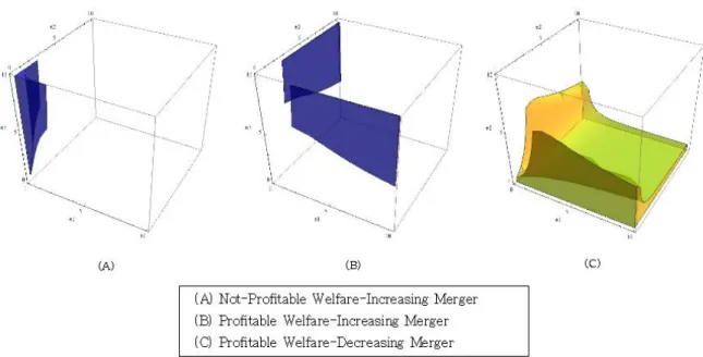
Table 2.2: Profitability and Welfare Effect of Merger

Type of Merger Profitability Welfare Effect Note

Case 1 loss if M_N+1<0.8 negative S-S-R model

Case 2 benefit negative∗ worse than S-S-R in welfare

Case 3 benefit ifM ≥M∗ negative∗ worse than S-S-R if M ≥M∗

2.4 Asymmetric Increasing Marginal Cost Model

As I discussed in the introduction, the merger concept of the S-S-R and the identical constant marginal cost model is not realistic. In this section, I build up the asymmetric increasing marginal cost model where a merged entity has bigger size or better technology than its constituent firms. Having this model, I perform the merger analysis similar to Section 2.3. Since a merger in this model may create cost saving from synergies, merger analysis includes its price effect as well.

2.4.1 Model

This model also basically follows the S-S-R model except that the cost function is modified. Demand and Supply : I keep using linear demand curveP = 1−Q. There areN firms before merger. In order to deal with cost asymmetry, I will introduce cost function similar to the one used by Perry and Porter (1985), McAfee and Williams (1992), Rothschild (1999) and etc. :

Ci(qi) =

q2_i 2ei

, ei >0 (2.10)

So the marginal cost of firm i is a linear function M Ci₍_q

i) = q_ei_i, and increases as output

increases in this setting. Here, ei can be seen as efficiency coefficient or technology-adjusted

capital stock, and the S-S-R setting is a specific case that ei is infinity. In order to focus on

cost saving effect from reallocation or synergy effect of merger, I assume that there is no fixed cost in this model.

(30)

analyze the incentive and welfare effect of a merger that creates synergy effect.

Merger Scenario : I will consider a 2-firm merger between firm 1 and firm 2 in this section. Two types of cost saving are analyzed : rationalization and synergy effect. Following the definition of Farrell and Shapiro (1990), rationalization model deals with the case that “the combined entity can better allocate outputs across facilities but its production possibilities are no different from those of the insiders (jointly) before the merger”. In fact, the merger concept in the Perry-Porter or McAfee-Williams model exactly coincides with rationalization. On the other hand, synergy effect model looks at the situation where the merged firm’s production possibilities are better than those of the constituent firms. Economies of scale or learning effect can be sources of synergy effect.

Firms’ Competitive Behavior: In this model, I assume firms compete`a laCournot pre-and post-merger like the S-S-R model. So I rule out the collusive effect as a motive of merger. There is no entry nor exit in this section.

I can derive Cournot-Nash equilibrium when there are N firms. Each firm i solves the following profit maximization problem:

πi(q) = (1−

N

X

k=1

qk)qi−

q2_i 2ei

, where q = (q1,· · ·, qN) (2.11)

Let me denoteλk= ₁₊ek_e_k.Then, Cournot-Nash equilibrium output and price are given by

Q∗_N =

PN

k=1λk

1 +PN

k=1λk

(2.12)

P_N∗ = 1

1 +PN k=1λk

(2.13)

and each firm i’s output and market share amount to

q_i∗ = λi 1 +PN

k=1λk

(2.14)

s∗_i = λi PN

k=1λk

(31)

Asei gets bigger, firm i’s market share becomes higher. Then, each firm’s profit yields

π∗_i = λi(1 +λi) 2(1 +PN

k=1λk)2

(2.16)

2.4.2 Analysis of Merger with Rationalization Effect

Having the equilibrium output, price and profit of each firm, I can analyze the incentive and welfare effect of a merger with rationalization. To this end, I need to derive cost function of a merged entity. In order to minimize its cost, the merged firm solves

min

q1,q2 q2₁ 2e1

+ q

2 2

2e2

subject to qM =q1+q2

So, its cost function becomes C1+2(qM) = q2

M

2(e1+e2). Note that the merged firm’s efficiency is equal to the sum of its constituent firms’ efficiency when a merger brings cost saving only from rationalization.

Incentive of Merger

Suppose that firm 1 and 2 merge, then a merged firm’s profit at post-merger Cournot-Nash equilibrium, denoted byπ_M1+2, would be

π_M1+2= λ1+2(1 +λ1+2) 2(1 +λ1+2+PNk=3λk)2

, where λ1+2=

e1+e2

1 +e1+e2

(2.17)

Then, the incentive of merger function,g_R1+2(e), is defined by using equation (2.16) and (2.17).

g1+2_R (e) = π_M1+2(e)−(π∗₁(e) +π₂∗(e)), where e= (e1,· · · , eN) (2.18)

= λ1+2(1 +λ1+2) 2(1 +λ1+2+PN_k₌₃λk)2

−λ1(1 +λ1) +λ2(1 +λ2)

2(1 +PN

k=1λk)2

So merger incentive depends not only on the merger participants’ efficiency (e1, e2) but also

on outsider’s efficiency (e3,· · · , eN).

(32)

Figure 2.6: Incentive of Merger - Rationalization

3 firms pre-merger (N = 3), theng_R1+2(e) yields

g_R1+2(e1, e2, e3) =π1+2_M (e1, e2, e3)−(π∗1(e1, e2, e3) +π2∗(e1, e2, e3)) (2.19)

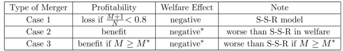
Figure 2.6 shows the space where a merger is profitable g_R1+2(e1, e2, e3)>0

when each firm’s efficiency takes a value between 0.1 and 10 (e1, e2, e3)∈[0.1,10]3

. Recall that any merger between 2 firms in triopoly market is not profitable under the S-S-R model becauseg1(3,1) =

1 9 −

1 8 = −

1

72 from equation (2.4). So, this example shows that “merger paradox” does not

always hold when cost saving from reallocation is possible.

Given that a merger may be profitable, the important question is how outsider’s or insiders’ efficiency affects the incentive of merger. We can get some intuitions from Figure 2.7. Panel (A) shows that any merger with rationalization is profitable when outsider’s efficiency level is low (e3 =.3). If outsider is efficient enough as in panel (B) and (C), however, there should be

an asymmetry in efficiency coefficients between constituent firms so that a merger is profitable (e3 = 1 or e3 = 5). Panel (B) and (C) also implies that the required asymmetry in efficiency

(33)

Figure 2.7: Outsider’s Efficiency and Incentive of Merger

Claim 4. Suppose that a merger is at least break-even at e = (e1,· · · , eN). If any outsider

gets more efficient, the merger becomes less profitable or unprofitable. (If g_R1+2(e) ≥ 0, then

∂ ∂ejg

1+2

R (e)<0 for j≥3.)8

It is useful to look at outsider’s response to a merger in order to understand this result. Using equation (2.13), (2.14) and (2.16), I can get the post-merger equilibrium price, outsider’s output and profit and can compare them with the equivalent pre-merger values.

P_N1+2 = 1

1 +λ1+2+PNk=3λk

> 1

1 +λ1+λ2+PNk=3λk

=P_N∗

q1+2_o = λo

1 +λ1+2+PNk=3λk

> λo 1 +PN

k=1λk

=q∗_o

π1+2_o = λo(1 +λo) 2(1 +λ1+2+PNk=3λk)2

> λo(1 +λo)

2(1 +λ1+λ2+PNk=3λk)2

=π_o∗

The inequalities comes fromλ1+λ2> λ1+2.Since the equilibrium price and outsider’s output

increase after a merger, the merged firm’s output q1+2_M should be less than the sum of its constituent firms’ pre-merger output q∗₁ +q∗₂. It depends on outsider’s efficiency how much the merged firm’s output decreases. To see that, note that λi = −dq_dQi from the first order

condition of (2.11). So, λi represents firm i’s responsiveness with respect to the change in

8_{A sufficient condition (g}1+2

R (e)≥0) is required to establish this result analytically, but numerically I could

(34)

market equilibrium output. Therefore, the more efficient an outsider is, the more it increases its output after merger because higherei is equivalent to higherλi. Big reaction of an efficient

outsider, in turn, harms the merged firm’s profitability.

Next, look at the relationship between cost asymmetry of constituent firms and the merger’s profitability. Note first that marginal costs are different among firms. From equation (2.14) and cost function, firm i’s marginal cost is given by M Ci(q_i∗) =h(1 +ei)

1 +PN

k=1λk

i−1 . So more efficient firm produces at lower marginal cost in Nash equilibrium. When 2 firms are combined by merger, the merged firm makes the marginal costs of these two facilities equal through reallocation of output in order to minimize its cost. Larger difference in merg-ing parties’ efficiencies is equivalent to larger difference in their marginal costs at pre-merger Nash equilibrium. So the merged entity can save more cost through reallocation. Formally, fix e1 +e2 = es and let e1 = (1−ν)es and e2 = νes for ν ∈ [0.5,1). Then asymmetry

between firm 1 and firm 2 comes to e2

e1 =

ν

1−ν, so larger ν is equivalent to bigger

asymme-try. Using (es, ν), I can redefine the incentive of merger function as g1+2_R (es, e3,· · · , eN, ν).

Then, I could show the following numerical result in the appendix: if a merger under N = 3 is not profitable, increase in asymmetry between insiders improves the incentive of merger

if g_R1+2(es, e3, ν)≤0, _∂ν∂ gR1+2(es, e3, ν)>0 f or all(es, e3)∈R2+

.

Welfare Effect of a Merger

As shown in previous subsection, a merger with rationalization increases price and out-siders’ output, while the merged firm’s output is lower than the sum of its constituent firms’ pre-merger output. So, this type of merger increases outsider’s profit and decreases consumer surplus. But merger’s profitability is not decisive. The merger’s overall effect on aggregate welfare depends on the relative magnitude of these 3 effects.

Since pre- and post-merger price and each firm’s profit have analytical solutions thanks to linear demand and marginal cost, welfare analysis can be performed directly. Given the characterization of pre- and post-merger Nash equilibrium, welfare effect of a merger yields

w_R1+2(e) =g_R1+2(e) +XN

k=3(π 1+2

k (e)−π

∗

k(e))−

Z P_N1+2(e)

P_N∗(e)

(35)

So the welfare effect of a merger depends on both the merger participants’ efficiency (e1, e2)

and outsiders’ efficiency (e3,· · ·, eN) as merger’s profitability does. It is not surprising

be-cause firms’ interaction affects consumer surplus and each firm’s profit in oligopoly mar-ket. With equation (2.20), I can check whether a merger is welfare-enhancing or not when e= (e1,· · ·, eN) is given. Moreover,ecan be identified from ₁₊ei_e_i = q

∗ i

P∗

N even when it is unob-servable. Using equation (2.13), (2.14), (2.20) with cost function, we can obtain the necessary and sufficient condition for welfare-increasing merger9

XN

k=1q ∗

kM Ck(q

∗

k)−qM1+2M C

1+2₍_q1+2

M )−

XN

k=3q 1+2

k M C k₍_q1+2

k )>(P

1+2

N )

2₋₍_P∗

N)2 (2.21)

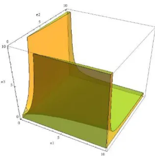
This condition says that the decrease in output-weighted marginal cost outweighs the increase in square of price in welfare-increasing merger. Because of the linearity of demand and marginal cost, half of left-hand side in condition (2.21) is equal to the decrease in total cost of the industry from the merger whereas half of right-hand side represents decrease in total revenue and consumer surplus. So, this condition requires that the industry’s profit increase from output rationalization outweighs decrease in consumer surplus under welfare-increasing merger. In order to see when this condition is satisfied in more detail, revisit the example where N = 3.Then, I can check the welfare effect of merger in the cubee∈[0.1,10]3 _{using equation}

(2.20). Figure 2.8 shows the space where a merger increases welfare (w_R1+2(e1, e2, e3) > 0).

This picture illustrates that a merger is more likely to increase social welfare if joint market share of merger participants is small and the outsider has the largest market share. Higher social welfare mainly comes from output reallocation between insiders and outsider in this case. Firm 3’s output increases after merger whereas aggregate output of firm 1 and 2 decreases. Since firm i’s marginal cost is equal to ₍₁₊_e 1

i)(1+λ1+λ2+λ3) in Nash equilibrium before merger, firm 3’s marginal cost is lowest if e3 is largest. Moreover, since larger e3 implies larger λ3,

firm 3 responds more to the decrease in aggregate output from merger. Therefore, a merger between small firms enables efficient outsider to produce more and relatively inefficient merged

(36)

Figure 2.8: Welfare Effect of Merger - Rationalization

entity to produce less, which makes it possible for social welfare to increase.10

On the other hand, Figure 2.8 shows that there is another type of welfare-enhancing merger, which combines a big firm and a small firm given the presence of a sufficiently efficient outsider. Output reallocation between insiders can be an additional source of higher welfare in this case. It happens because a merged firm can save its cost by increasing the output of the efficient participant and decreasing the output of the inefficient participant. So, the merger might enhance social welfare even when the efficient participant’s initial market share is larger than the outsider’s market share.

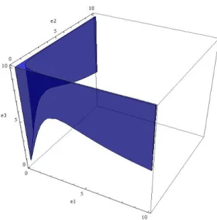
As shown in panel (A) of Figure 2.9, a merger between firms with small market share is rarely privately profitable although this merger may increase social welfare. So the second fea-ture of the S-S-R model may occur in a merger with rationalization. Since this kind of merger cannot benefit from cost asymmetry between participants by much, cost saving effect from

10

(37)

Figure 2.9: Profitability and Welfare Effect of Merger with Rationalization

reallocation is restricted for the merged entity. Moreover, the output response of efficient out-sider is big, which harms the merged firm’s profitability. So it is unlikely for a merger between small inefficient firms to occur in the market. In contrast, a merger is privately profitable and welfare enhancing when there is a sufficiently efficient outsider and a big asymmetry in cost efficiency between participants as is illustrated in panel (B). Asymmetry of insiders improves both profitability and welfare effect of merger while outsider’s response improves welfare but hurts merger’s profitability. Overall, the cost saving effect from big asymmetry outweighs profit loss due to outsider’s output increase in this case. Panel (C) in Figure 2.9 shows the space where a merger is profitable but welfare-decreasing. This is the type of merger which antitrust policy has to concern about because it is likely to occur but socially undesirable.

The fact that the welfare effect of a merger depends on outsider’s efficiency level and insiders’ asymmetry has some policy implication as well. A merger with the same efficiency combination (e1, e2) of participants might be either socially beneficial or harmful depending on

outsider’s efficiency level. Similarly, a merger with the same post-merger efficiencyes=e1+e2

(38)

2.4.3 Analysis of Merger with Synergy Effect

Merger models that I analyzed so far have adverse effects on consumer surplus because the equilibrium price increases after merger. It is quite a natural result from Proposition 2 of Farrell-Shapiro, which proves that a merger without synergy effect causes the equilibrium price to rise. Now I will move the scope of analysis to the type of merger creating synergy effect. For that purpose, I let the merged firm’s cost function as C1+2(qM) =

q2 M

2eM such that eM > e1+e2 holds. Here,eM represents the merged firm’s efficiency level.

Incentive of Merger

Given the merged firm’s cost function, its profit at post-merger Cournot-Nash equilibrium would be

π_M1+2= λM(1 +λM) 2(1 +λM +PNk=3λk)2

, whereλM =

eM

1 +eM

(2.22)

Then, using arguments similar to those in the rationalization case, the incentive of merger function, denoted byg_S1+2(e, eM), becomes

g1+2_S (e, eM) = πM1+2(eM, e3,· · · , eN)−(π1∗(e) +π2∗(e)), where e= (e1,· · · , eN) (2.23)

= λM(1 +λM) 2(1 +λM +PNk=3λk)2

−λ1(1 +λ1) +λ2(1 +λ2)

2(1 +PN

k=1λk)2

Now the incentive of merger depends on the magnitude of synergy effect besides the insiders’ and outsider’s efficiency level. Then, the relationship between the magnitude of synergy effect and the incentive of merger can be derived.

Claim 5. A merger’s profitability improves as synergies get stronger.

g_S1+2(e, eM)> gR1+2(e) is immediate from this Claim. I can obtain some economic rationale

of this result from the comparison between a merged firm’s output in a rationalization merger, denoted byq_M1+2, and that in the equivalent merger with synergies, denoted byq1+2_M (eM). From

equation (2.14), q_M1+2and q_M1+2(eM) are given by

q_M1+2= λ1+2

1 +λ1+2+PNk=3λk

< λM

1 +λM +PNk=3λk

(39)

The inequality comes from λM > λ1+2. The equilibrium output of the merged firm becomes

larger as synergy effect gets stronger. In contrast, outsider’s output in a rationalization merger is higher than that in an equivalent synergy effect merger q1+2_o > q1+2_o (eM)

. Hence, the presence of synergy effect restricts the amount of outsider’s output response after merger, which in turn improves the merger’s profitability. For the same reason, outsider’s post-merger profit, or equivalently “free rider’s problem” proposed by J.Stigler, gets smaller with the stronger synergy.

π_o1+2= λo(1 +λo) 2(1 +λ1+2+PN_k₌₃λk)2

> λo(1 +λo) 2(1 +λM +PN_k₌₃λk)2

=π_o1+2(eM) (2.24)

Welfare Effect of Merger

The post-merger equilibrium price is given by

P_N1+2(eM) =

1

1 +λM+PN_k₌₃λk

(2.25)

While the effect of merger on consumer and outsider is not decisive, equation (2.24) and (2.25) imply that higher synergy lowers post-merger equilibrium price and outsider’s profit. Given these equations, welfare effect of a merger with synergy effect yields

w_S1+2(e, eM) =g_S1+2(e, eM) + N

X

k=3

(π1+2_k (eM)−π∗k(e))−

Z P1+2

N (eM)

P_N∗(e)

(1−P)dP (2.26)

As in the incentive of merger, the welfare effect depends on the magnitude of synergy effect in addition to the insiders’ and outsider’s efficiency level. Using equation (2.13), (2.14) and cost function, I can transform equation (2.26) into the necessary sufficient condition for welfare-increasing merger (w_S1+2(e, eM)>0).

N

X

k=1

q∗_kM Ck(q_k∗)−q_M1+2(eM)M C1+2(q1+2M (eM))− N

X

k=3

q_k1+2(eM)M Ck(q_k1+2(eM))

(40)

Figure 2.10: Welfare Effect of Profitable Merger - Synergy

Condition (2.27) is similar to condition (2.21), but each term (q_M1+2(eM), M C1+2(q1+2M (eM)),

q_k1+2(eM), M Ck(qk1+2(eM)) andPN1+2(eM)) has a different value from rationalization case and

varies depending on the level of synergy. Using equation (2.26), we can derive the relationship between the magnitude of synergy effect and the welfare effect of merger.

Claim 6. A merger’s welfare effect improves as synergies get stronger if and only ifeM satisfies

eM >

−1−2PN

k=3

λ2 k

ek +

PN

k=3λk

4 + 2PN

k=3

λ2 k

ek +

PN

k=3λk

(2.28)

Claim 6 shows that stronger synergy always improves merger’s welfare effect for N = 3, and it does for N ≥ 4 unless eM is too small. In order to compare with rationalization type

merger, let me consider the case ofN = 3 again.Since synergy effect improves both a merger’s profitability and welfare effect in this case, it expands the scope for privately profitable and socially desirable mergers.

Suppose 10% of synergy effect (i.e. eM = 1.1∗(e1+e2)).The shaded space in panel (A) of

(41)

Figure 2.11: Synergy Effect and Profitability of Welfare-Increasing Merger

2.9, so mergers with synergy are profitable and welfare-enhancing in wider range. In fact, the blue shape includes all the unprofitable welfare-increasing mergers without synergy (panel (A) of Figure 2.9) as well. The profitability of a merger with synergy improves not only because the merged entity can save its cost from both reallocation and synergy, but also because the enhanced productivity of the merged firm restricts outsider’s output increase post-merger.

It is also worthwhile to note that there still exist profitable welfare-decreasing mergers with 10% synergy from panel (B) in Figure 2.10. This yellow shape do not disappear even with stronger synergy effect, say 100%. So the presence of strong synergy effect is not sufficient for welfare to increase after merger.

(42)

Synergy Effect of Merger and Consumer Surplus

Farrell-Shapiro’s Proposition 1 provides a necessary and sufficient condition for a merger to improve consumer surplus. When two firms merge, the condition comes to M C1(q∗₁) −

M C1+2(q∗₁+q∗₂) > P_N∗ −M C2(q₂∗). Given the functional form of demand and cost function, this condition boils down to the following result.

Claim 7. [Farrell-Shapiro] A merger improves consumer surplus if and only if

λ1+λ2 < λM (2.29)

There are two things to note on this Claim. First, it only depends on insiders’ efficiency and the magnitude of synergy whether a merger is CS-increasing or not, which is in contrast with welfare effect of merger. More surprisingly, if the constituent firms of a merger are efficient enough in the sense that λ1 +λ2 > 1, then the merger cannot improve consumer surplus

irrespective of the magnitude of its synergy effect. Using Claim 7, I can check the profitability of any CS-increasing merger.

Claim 8. Any CS-increasing merger is profitable for merging firms.11

Claim 8 is also in contrast with a welfare-increasing merger, which is not always profitable. This result holds because sufficient synergy effect is required for a merger to improve consumer surplus. But the inverse is not true because a profitable merger is not necessarily CS-increasing. This model confirms the well-documented fact that a merger increases consumer surplus if and only if outsider’s profit decrease. [Stillman (1983), Farrell and Shapiro (1990), Duso, Neven, and Roller (2007), etc.] To see this, using equation (2.16) yields

π1+2_o (eM) =

λo(1 +λo)

2(1 +λM +PNk=3λk)2

< λo(1 +λo)

2(1 +λ1+λ2+PNk=3λk)2

=π_o∗

11

Claim 8 holds in a very general setting. This result only requires the following two conditions, which Farrell and Shapiro (1990) assumes. See the appendix.

Condition 3 : p0(Q) +qip00(Q)<0, i= 1,· · ·, N

Condition 4 : _dqd22 i

(43)

Table 2.3: The Welfare Effect of Horizontal Merger Type of Merger Insiders Outsiders Consumer Net Effect 1. CS-decreasing non-definite benefit loss non-definite

2. CS-neutral benefit neutral neutral positive

3. CS-increasing benefit loss benefit positive

Here,π_o1+2(eM) represents the outsider o’s post-merger profit whereasπ∗odenotes its pre-merger

profit, and the inequality comes from λ1 +λ2 < λM. So, “free rider’s problem” completely

disappears in a CS-neutral and CS-increasing merger. Further, a CS-increasing merger reduces outsider’s output and its market share as well. Denote the outsider’s pre-merger output and market share by q_o∗ and s∗_o, and its post-merger output and market share by q1+2_o (eM) and

s1+2

o (eM). From equation (2.14) and (2.15), I can obtain

q_o1+2(eM) =

λo

1 +λM +PN_k₌₃λk

< λo 1 +PN

k=1λk

=q∗_o

s1+2_o (eM) =

λo

λM+

PN k=3λk

< _P_Nλo

k=1λk

=s∗_o

Again, the inequality comes from λ1+λ2 < λM. Therefore, the merged firm’s market share

gets larger than the joint pre-merger market share of its constituent firms in a CS-increasing merger.

Using these results enables me to check the welfare effect of a CS-neutral merger. Any CS-neutral merger does not affect consumer surplus by definition, nor the outsiders’ profit. So the welfare effect of CS-neutral merger is simplified intow_S1+2(e, eM) =gS1+2(e, eM). The proof

of Claim 8 shows that a CS-neutral merger is profitable, so it is welfare increasing.

Table 2.3 summarizes the discussion so far on the profitability and welfare effect of a merger. The profitability of CS-decreasing merger is not decisive but improves as insiders are more asymmetric, outsiders are “less” efficient and the merger creates bigger synergies while CS-neutral or CS-increasing merger is profitable.

(44)

in the S-S-R model or rationalization type merger is also always CS-decreasing, so outsiders benefit from both kinds of merger.

The welfare effect of CS-decreasing merger is not decisive but improves as insiders are “smaller” or more asymmetric, outsiders are “more” efficient and the merger creates bigger synergies whereas CS-neutral or CS-increasing merger is welfare-increasing in general.12

2.4.4 One Merger’s Effect on Another Merger’s Profitability

The comparative statics in this subsection is how one merger affects another merger’s profitability. If a merger enhances the profitability of another merger(s), then mergers are more likely to occur simultaneously or in chain, which is called “merger wave”.

To deal with this issue, it is useful to rewrite g_S1+2(e, eM) in (2.23) using y ≡ PN_k₌₃λk.

Then, the incentive of merger function becomes

g1+2(e1, e2, eM, y) =

λM(1 +λM)

2(1 +λM +y)2

−λ1(1 +λ1) +λ2(1 +λ2)

2(1 +λ1+λ2+y)2

Besides a merger between firm 1 and 2 (merger A), let me consider another merger between firm 3 and 4 (merger B) without loss. After merger B,y comes toy0=λ0_M +PN

k=5λk, where λ0_M = e

0 M

1+e0_M and e

0

M represents the efficiency level of the merged firm coming from merger

B. Claim 7 implies that y decreases (increases) if and only if merger B is CS-decreasing. (CS-increasing, resp.) Taking a partial of g1+2(e1, e2, eM, y) with respect toy, I can obtain

∂ ∂yg

1+2₍_e

1, e2, eM, y) =

λM(1 +λM)

(1 +λM +y)2

[ 1

1 +λ1+λ2+y

− 1

1 +λM +y

]

−2g

1+2₍_e

1, e2, eM, y)

1 +λ1+λ2+y

(2.30)

Equation (2.30) brings me the following result.

Claim 9. Suppose that merger A is break-even without merger B. Another CS-decreasing

merger B may trigger the occurrence of merger A.

12

(45)

This Claim provides a sufficient condition where a merger becomes more profitable after the occurrence of another CS-decreasing merger: g1+2(e1, e2, eM, y)≥0 andλ1+λ2 ≥λM.Since

this is a sufficient condition, even unprofitable mergers may turn profitable after the occurrence of another CS-decreasing merger. To see this, suppose that merger A is unprofitable before merger B happens. Then λ1+λ2> λM and g1+2(e1, e2, eM, y)<0 hold. If the loss of merger

A is small enough, _∂y∂ g1+2(e1, e2, eM, y)<0 holds from equation (2.30). So it can be the case

thatg1+2(e1, e2, eM, y0)>0.

The reason why this Claim holds is again related to the output response of outsiders. Without merger B, merger A causes firm 3 and 4 to adjust their output individually. But if firm 3 and 4 are combined by merger B, this merged entity will best respond to the change in aggregate output caused by merger A. Since merger B is CS-decreasing, λ3+λ4 > λ0_M holds.

Recall that λi is firm i’s responsiveness with respect to the change in market equilibrium

output. So, the merged entity’s output response is smaller than the joint output response of firm 3 and 4 for a given aggregate output change. Hence, the presence of a CS-decreasing merger reduces the output response of outsider(s), which improves the profitability of a merger between firm 1 and 2. Claim 9 and this discussion partly explains why mergers are apt to occur simultaneously or in chain.

2.4.5 General Linear Demand and Merger Analysis

In order to analyze the effect of demand side on profitability and welfare effect of merger, I will assume P =a−bQ in this subsection, where a >0 and b > 0. So, a is related to the market size whilebis related to elasticity. If I do the same exercise with this demand function, the incentive of merger function, denoted byg1+2₍_{e, e}

M, a, b), comes to

g1+2(e, eM, a, b) =

a2 2b[

µM(1 +µM)

(1 +µM +PN_k₌₃µk)2

−µ1(1 +µ1) +µ2(1 +µ2)

(1 +PN

k=1µk)2

], (2.31)

where _µ_M ₌ beM

1+beM and µk=

bek 1+bek

Note that if eM = e1 +e2 and a = b = 1, g1+2(e, eM, a, b) = g1+2(e, e1+e2,1,1) = g_R1+2(e)

(46)

g1+2_S (e, eM) in equation (2.23). The change in outsider o’s profit from the merger yields

π1+2_o −π∗_o =a

2

2b[

µo(1 +µo)

(1 +µM +PNk=3µk)2

− µo(1 +µo)

(1 +PN

k=1µk)2

]

Since pre-merger and post-merger Nash equilibrium price is given by

P_N∗ = a 1+PN

k=1µk

, P_N1+2= a

1 +µM+PNk=3µk

, (2.32)

the welfare effect of merger, denoted byw1+2(e, eM, a, b), comes to

w1+2(e, eM, a, b)=g1+2(e, eM, a, b)+ N

X

k=3

(π1+2_k −π_o∗)−1

b

Z P_N1+2

P∗ N

(a−P)dP (2.33)

Similarly, if eM = e1+e2 and a =b= 1, w1+2(e, eM, a, b) =w1+2(e, e1+e2,1,1) =wR1+2(e)

in equation (2.20) and if eM > e1+e2 and a=b= 1, w1+2(e, eM, a, b) =w1+2(e, eM,1,1) =

w1+2_S (e, eM) in equation (2.26). Equation (2.31), (2.32), and (2.33) give the following result,

immediately.

Claim 10. (a)g1+2(e, eM, a, b) = a

2

b g1+2(be, beM)

(b) w1+2(e, eM, a, b) = a

2

b w

1+2₍_{be, be}

M)

(c) A merger improves consumer surplus if and only if µ1+µ2 < µM.

So, g1+2(e, eM, a, b) > 0 is equivalent to g1+2(be, beM) > 0, as is w1+2(e, eM, a, b) > 0

equivalent to w1+2(be, beM) >0.Then, while market size variable aaffects the magnitude of

merger’s profitability and welfare effect, it relies only on (e, eM, b) whether a merger is profitable

or welfare-increasing. In addition, it only depends on (e1, e2, eM, b) and not on market size

variableawhether a merger is CS-increasing. Hence, Claim 10 shows that qualitative merger analysis can be done with demandP = 1−Qif I substitute (e, eM) with (be, beM) even when

the real demand isP =a−bQ.

Note that (e, eM, b) is all the information requirement for the qualitative welfare analysis of

a merger whereas (e1, e2, eM, b) is required for the qualitative price effect analysis of a merger.