INHOMOGENEOUS BRANCHING PROCESSES: A TALE OF TWO NETWORKS
Jimmy Jin
A dissertation submitted to the faculty of the University of North Carolina at Chapel Hill in partial fulfillment of the requirements for the degree of Doctor of Philosophy in the
Department of Statistics and Operations Research.
Chapel Hill 2017
c
2017
Jimmy Jin
ABSTRACT
JIMMY JIN: Inhomogeneous Branching Processes: A Tale of Two Networks (Under the direction of Shankar Bhamidi and Andrew Nobel)
ACKNOWLEDGEMENTS
This is the most difficult portion of the thesis to write. I truly believe that everyone I have ever met played some role—however imperceptible—in setting me along the path which led to this thesis. I thank you all. But still, there are some who are more deserving of thanks than others.
Obviously, my family is at the top. A paragraph cannot possibly sum up their contribu-tion. I can say this much though: since a very young age, I’ve been very curious. I was never the smartest, the most knowledgeable, or even the most hard-working. What’s carried me this far is simply my ever-present desire to peek around the next corner. For fostering and preserving that spirit within me, I thank my mom, dad, and sister. To this day, the same curiosity still guides me ever forward.
In the same vein, I thank all of my teachers over the years. Special thanks are due to two of my wonderful math professors at Swarthmore College: To Phil Everson, who showed me that statistics is really just fancy guessing and that fancy guessing is actually quite fun; and to Deb Bergstrand, who more than anyone else helped me glimpse the beauty in the most abstract corners of mathematics. I’ll always remember that first sense of wonder I felt as you were explaining why permutations cannot be both even and odd.
Next I would like to thank my advisors Andrew and Shankar. I won’t dwell on how they trained me technically—that’s a baseline requirement for any worthwhile advisor. For me, Andrew and Shankar’s contribution was far deeper. Let me explain.
wake up in the morning and feel excited about contributing to such a system. I began to wonder whether the true spirit of scientific discovery was still alive out there, or whether we were all eventually just going to end up going through the motions, chasing the next hot topic which will garner us the most citations. I started to worry that my passion for research would someday wane and that I would end up just another cog in a giant paper mill.
You see, this ennui is a disease which strikes at the heart of scientific progress. Once a researcher, no matter their raw talent, loses the capacity to dream—to see their work as something more than just a job—then they end up as part of the problem. They spend the rest of their lives chasing prestige, citations, or the next cozy job title rather than the thing that got them in the game in the first place: the pleasure and excitement of discovering.
Therefore, I believe the true measure of a successful advisor is not their ability to train the student in technical matters but rather their ability to inspire in the student a deep appreciation and enjoyment in the work that they do. The benefits of good technical advice is short-lived. The benefits of a healthy passion for research last an entire lifetime.
For me, Shankar and Andrew succeeded in this wonderfully. It’s difficult to put a finger on exactly what they did. But whether it was their willingness to work with me on topics far afield of their expertise, or the example they set from their own passion for tackling problems, the end result is that I always felt inspired and excited about learning and exploring. And that, in turn, is what kept me going even when I felt like the system was so broken that there was no point in keeping on. I can’t thank them enough for that.
Thanks are also due to many individuals in my life who don’t fit neatly into a category: • To my classmates Kelly, John, Qunqun, and Ruoyu, whose positivity and humor made the Hanes basement as pleasant a place to be as it could possibly be (please don’t forget about me when you’re wealthy and/or successful).
• To the power trio of Alison, Sam, and Christine, who made it possible for the rest of us to keep our heads in the clouds by taking care all the stuff that keeps us connected to the ground.
• To Iain Carmichael, for hooking me up with the CourtListener data.
• To Kyle Skolfield for helping to read my thesis and ensure that there isn’t too much stupidity contained within.
• To Shankar’s dog Annabelle, for being really cute and not trying to eat me.
• To my cat Peachy, who surely can’t read but definitely is the best stress-relieving device to ever appear on this planet.
• To Alex Valencia, for also putting with me for that one time I squatted in your house. Also Yue, and also for introducing me to. . .
• ...and lastly but not least, to Diana, who more than anyone else remind s me that there is much joy to be had outside of math and statistics. And that I need to eat more vegetables. I would not have made it here without you.
TABLE OF CONTENTS
LIST OF TABLES . . . xii
LIST OF FIGURES . . . xiii
LIST OF ABBREVIATIONS AND SYMBOLS . . . xvi
1 Introduction . . . 1
1.1 Summary of thesis . . . 2
1.1.1 Preferential attachment with change point . . . 2
1.1.2 Decreasing cascades and thinned branching processes . . . 7
2 Background and literature . . . 11
2.1 The growth of branching populations . . . 11
2.1.1 The Dummies’ guide to the Kesten-Stigum theorem . . . 11
2.1.2 Inhomogeneous and infinite-mean processes . . . 14
2.1.3 Continuous time branching processes . . . 18
2.2 Networks . . . 23
2.2.1 Scale-free networks . . . 23
2.2.2 Preferential attachment . . . 25
2.2.3 Changepoint detection on networks . . . 29
2.3 Cascades . . . 32
2.3.1 What is a cascade? . . . 32
2.3.2 The shape of viral cascades . . . 35
3 Changepoint detection on preferential attachment . . . 38
3.1.1 Organization . . . 39
3.1.2 Model formulation . . . 39
3.1.2.1 Model with change point . . . 41
3.1.3 Preliminary notation . . . 41
3.2 Results . . . 43
3.2.1 Asymptotics for the degree distribution . . . 43
3.2.2 Change point detection . . . 44
3.3 Discussion . . . 50
3.3.1 Change point detection literature . . . 50
3.3.2 The asymmetry within the scaling (1−t) . . . 51
3.3.3 Multiple change points . . . 54
3.3.4 Existing work regarding preferential attachment . . . 56
3.3.5 Proof techniques . . . 57
3.3.6 Empirical dependence of the convergence on parameter values . . . 58
3.4 Proofs . . . 59
3.4.1 Preliminaries . . . 60
3.4.2 Convergence of the degree distribution . . . 68
3.4.2.1 Overview of the proof . . . 68
3.4.2.2 Analysis of ¯NnBC(·) : . . . 70
3.4.2.3 Analysis of ¯NAC n (·) : . . . 73
3.4.3 Proof of the tail exponent for the limiting degree distribution . . . 83
3.4.3.1 Overview of the proof . . . 83
3.4.3.2 The upper bound . . . 84
3.4.4 Analysis of the maximal degree . . . 86
3.4.5 Analysis of the proportion of leaves . . . 90
3.4.5.1 Expectation error bounds . . . 91
3.4.6 Consistency of the estimator . . . 98
4 Changepoint: simulations and analysis of real data . . . 100
4.1 Introduction . . . 100
4.2 Change point: further notes and simulations . . . 101
4.2.1 Preferential attachment: the role of functions . . . 101
4.2.2 The behavior of ˆγ in simulations . . . 103
4.2.2.1 The bias-variance tradeoff in . . . 103
4.2.2.2 The bias-variance tradeoff inω . . . 104
4.2.3 Performance of the estimator on trees . . . 108
4.2.3.1 Performance vs. the true change point γ . . . 108
4.2.3.2 Sensitivity of ˆγ with regards to |α−β|. . . 110
4.2.4 Extension of ˆγ to graphs with m >1 . . . 112
4.2.4.1 The function Dn(k)(t) . . . 112
4.3 Real data . . . 115
4.3.1 The raw data . . . 117
4.3.1.1 The arXiv graph . . . 117
4.3.1.2 The CourtListener graph . . . 118
4.3.2 Does it look like preferential attachment? . . . 119
4.3.2.1 The arXiv graph . . . 119
4.3.2.2 The CourtListener graph . . . 122
4.3.3 Analysis of the network history . . . 125
4.3.3.1 The time scale of real life . . . 126
4.3.3.2 The large hadron collider? . . . 127
4.3.3.3 The 4th and 9th circuit courts . . . 131
4.4 A note about code . . . 134
5 Decreasing cascades on scale-free graphs . . . 136
5.1 Introduction . . . 136
5.2 A cascade by a branching process . . . 138
5.2.1 Decreasing cascades . . . 139
5.2.2 The branching processes approximation on a graph . . . 141
5.2.3 Coupling to a graph: a sketch . . . 145
5.3 Analysis of the branching process . . . 146
5.3.1 The thinned branching process . . . 146
5.3.2 The extinction criteria . . . 148
5.3.3 Proof of Theorem 5.3.3 . . . 151
6 Future directions . . . 157
6.1 Changepoint . . . 157
6.1.1 Timing . . . 157
6.1.2 Non-linear attachment . . . 157
6.1.3 Preferential attachment with types . . . 159
6.2 Cascades . . . 160
6.2.1 The growth of the supercritical thinned branching process . . . 161
6.2.2 Shape . . . 164
6.2.3 Inference for the virality of a cascade . . . 164
LIST OF TABLES
LIST OF FIGURES
1.1 The evolution of a preferential attachment graph with change point at
γ = 0.4. . . 4
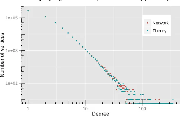
3.1 Log-log plot of the limiting degree distribution (red) and simulated net-work degree distribution (blue) with netnet-work size n = 500,000 and a corresponding sample of the same size from the predicted degree distri-bution. The model parameters are taken as α= 6, β= 1 and the change
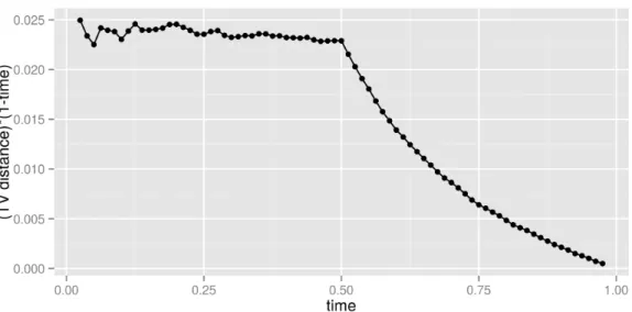
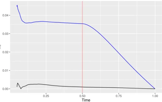
point γ = 0.5. . . 45 3.2 The functionDn(t) with network sizen= 200,000, and model parameters
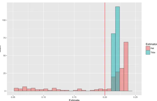
α = 6, β = 1 and the change pointγ =.5 as in Figure 3.1. . . 50 3.3 Histograms of ˜γ vs. ˆγ for a change point of α= 0 to β = 10 atγ = 0.20
(N = 100,000 vertices). . . 52 3.4 γ˜ vs. ˆγ for a change point of α = 0 to β = 10 at various values of γ
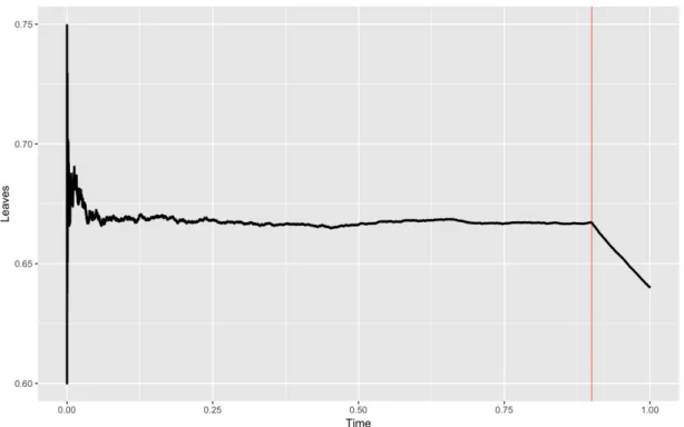
(N = 100,000 vertices). . . 53 3.5 The proportion of leaves in a PA graph on N = 100,000 vertices with
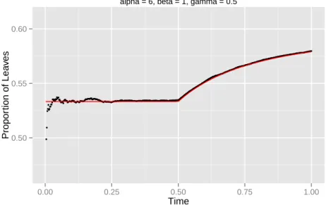
change point at γ = 0.9 from α= 0 to β = 10. . . 53 3.6 Empirical proportion of leaves in a simulation with n = 200,000, α =
6, β = 1, γ = 0.5. The red line represents the theoretical predictions in
(3.10). . . 58 3.7 Empirical proportion of leaves in a simulation with n = 200,000, α =
6, β = 5, γ = 0.5. The red line represents the theoretical predictions in
(3.10). . . 59 3.8 The process BPα(·) in continuous time starting from the root ρ and
stopped at τ15. . . 61
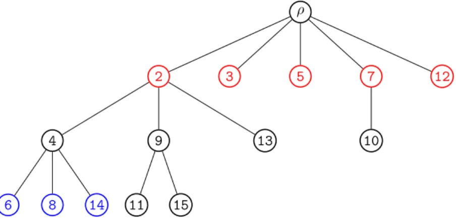
3.9 The corresponding discrete tree containing only the genealogical
infor-mation of vertices in BPα(τ15). . . 61
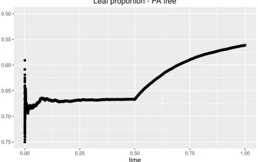
4.1 The proportion of leaves in a preferential attachment tree with γ = 0.5,
α = 0 andβ = 10. . . 102 4.2 Plot of Dn(t) for the with-changepoint model (blue) versus the
no-changepoint model (black) . . . 103 4.3 Illustration of when the log(n)/√n threshold (indicated by pink box)
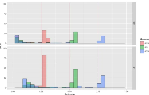
4.4 The effect of increasing from 0.01 to 0.10 for γ ∈ {0.25,0.50,0.75}.
ω = log in both cases. . . 105 4.5 Effect of not normalizing Dn(t) by maxtDn(t) on a graph withγ = 0.5,
α = 0, β = 10, and N = 500,000. The red tube is the unnormalized
threshold with vertical line at the estimate ˆγ. . . 106 4.6 Normalized vs. unnormalized estimates for a change point of α = 0 to
β = 10 at various values of γ. . . 107 4.7 γ vs. ˆγ for various γ ∈ [0.05,1.00]. Changepoint is α = 0 to β = 10 on
N = 100,000 vertices with = 0.05 and ω= log. . . 108 4.8 Plots of Dn(t) with (blue) and without (black) the scaling (1−t), for
N = 100,000 vertices and γ = 0.9, α= 0,and β= 10. . . 109 4.9 Histograms of ˆγ for γ = 0.9 with = 0.05 (top) and= 0.50 (bottom). . . 110 4.10 Histogram of estimates ˆγ ofγ = 0.5 with various separations|α−β|with
(α+β)/2 = 5 andN = 100,000 in all cases. Blue line indicates the mean estimate.111 4.11 The proportion of degree-4 vertices in a preferential attachment graph
with m = 4 with changepoint atγ = 0.5 (blue) and without changepoint (black). 113 4.12 Plot of Dn(1) for a preferential attachment tree with m= 1 vs. Dn(4) for a
graph with m= 4 on N = 100,000 vertices with change point atγ = 0.5
from α= 0 to β = 10. Dashed lines indicate argmaxes. . . 114 4.13 Log-log degree distribution for selected arXiv categories. . . 120 4.14 Time series of initial out-degree of per paper for selected arXiv categories,
smoothed by moving average over 2000 papers. . . 122 4.15 Log-log degree distribution for selected courts. . . 123 4.16 Time series of initial out-degree of per paper for selected appellate courts,
smoothed by moving average over 1000 cases. . . 125 4.17 Distribution of paper appearance times in arXiv categorieshep-ph versus math. . . 127 4.18 comparison of the initial out-degree series for arXiv categorymathplotted
on the order-based time scale (top) versus the real-life time scale (bottom). . . 128 4.19 Initial out-degree for the hep-ph category, moving average over 3000
pages. Red line indicating March 30, 2010. . . 129 4.20 Proportion of degree-15 vertices in the hep-ph category. Red line
4.21 Average degree of top-3 out-neighbors, moving average over 1000 vertices.
Red line indicating March 30, 2010. . . 131 4.22 Initial out-degree of court case citations from the 4th and 9th Circuit
Court of Appeals, smoothed over 1000 cases. Red line at January 1,
2000 for reference.. . . 132 4.23 Distribution of citation appearance times. Red lines at January 1, 2000
LIST OF ABBREVIATIONS AND SYMBOLS
pθ limiting degree distribution of the preferential attachment graph driven by the parameter set θ = (α, β, γ).
Dθ random variable with the distribution pθ, defined in 3.7.
Doutθ Dθ −1, representing a random variable with the limiting out-degree dis-tribution.
BC,AC before-changepoint, after-changepoint
Pα(Pβ) the Yule-process variant driven by parameter α (β) viewed as a point process, defined in 3.4.
Nα(t)(Nβ(t)) number of points in Pα (Pβ) which fall in the interval [0, t].
Tθ,n(Tn) preferential attachment (random) tree on n vertices driven by parameter set θ.
th(n) average proportion of leaves in the graph on n vertices over all times up to t, see 3.21.
h(n)
t average proportion of leaves in the graph on n vertices over all times after t, see 3.22.
Dn(t) scaled absolute difference between th(n) and h
(n)
t , see 4.2. D(t) theoretical limit of Dn(t) as n→ ∞, see 3.106.
p(∞)
t the limiting proportion of leaves in the graph as t→ ∞ as a function of t. Nn(k) number of vertices with degree k in the random tree Tn.
Nn(k, m) number of vertices with degree k in the random tree Tn at the time of appearance of the mth vertex.
ˆ
Nn(k, t) number of vertices with degree k in the random tree Tn at time nt. ˆ
pn(k, t) proportion of vertices with degree k in the random tree T
n at timent. ˆ
pn
t := ˆpn(1, t), or the proportion of leaves in the random tree Tn at time nt.
BPα(t) continuous-time branching process embedding of the preferential attach-ment graph driven by parameter α, see 3.4.1.
|BPθ(t)| number of individuals in BPθ(t) at time t.
Υn amount of time after the change point until the process reaches size n in the continuous-time embedding of the preferential attachment with change point model.
a limiting expectation of Υn, equal to 1/(2 +β) log(1/γ).
Age the age (in the continuous-time embedding of preferential attachment) of a vertex born after the change point by the time the process reaches its final size.
kn(s) cumulant generating function for the offspring of an individual in genera-tion n.
k(n)(s) nth functional iterate of the cumulant generation functions {k
m}06m<n. hn(s) functional inverse of kn(s).
CHAPTER 1 Introduction
In the theory of random graphs, most of the answers can be guessed using the heuristic that the growth of the cluster is like that of a branching process.
-Rick Durrett, Random Graph Dynamics
Graphs and networks are more relevant than ever. Whether in statistics, computer science, physics, or economics, the random graph has seen its role come front and center in the past decade as the world has grown more interconnected. For the statistician or probabilist, this is both the best of times and the worst of times. Best—because of an explosion of real-world data with which to drive new ideas and models. But also worst— because real-world phenomena does not always fit into neat, simplified mathematical models. Increasingly, we are preoccupied with inventing better, more accurate models to fit what we observe in reality.
However, this thesis is not an effort to do that. The reader will find no pretense in this thesis of claiming to outperform an existing method for modelling a network or for estimating some parameter of a stochastic block model. Rather, it is a testament to the power of a simple tool, the humble branching process, to achieve deep insights. In this thesis, we show that this simple stochastic process, familiar to any sufficiently advanced undergraduate, can reveal deep insights when properly employed.
Theorem (2.4.1). Suppose we have an Erd˝os-R´enyi random graph with λ > 1. If we pick two points at random from the giant component, then
d(x, y) logn →
1
logλ in probability.
The explanation for the theorem was the following:
The answer in Theorem 2.4.1 is intuitive. The branching process approximation grows at rate λt, so the average distance is given by solving λt = n, i.e., t = (logn)/logλ.
To someone completely new to random graph theory working through a book clearly written for other probabilists, seeing a familiar structure like branching processes is like happening across a road after being lost in the woods for several days. Branching processes became a path which the author could follow to delve deeper into random graph theory without fear of losing his way.
And to the author’s surprise, they have never stopped serving that purpose. Indeed, if one squints hard enough, branching processes can be found in many random graph models. In this thesis, we explore two important topics in random graph theory through the lens of branching processes.
1.1 1.1. Summary of thesis
1.1 1.1.1. Preferential attachment with change point
Question: Suppose we have a network growing over time, controlled indirectly by a parameter governing how new nodes join the network. If that parameter experiences a sudden change, how can we estimate it?
which is simple, yet capable of producing many characteristics seen in real-world graphs— namely, a power-law degree distribution. We propose a simple change point variant of this model, investigate some non-trivial ramifications, and then show how one can estimate the change point.
The basic preferential attachment graph is grown by the following scheme:
Start with a single vertex ρ at time m= 1 (this vertex will be referred to as the root or the original progenitor of the process). Fix a parameterα >−1. At each discrete-time point 1 < m 6 n a new vertex enters the system with a single edge1 which it will then connect to a pre-existing vertex. The vertex connects to a pre-existing vertex v with probability proportional to the current degree of v +α.
Now consider the same model but with a change point in the attachment parameter α. Fix two attachment parameters α, β > −1, a change point parameter γ ∈ (0,1), and a system sizen >1. The model does preferential attachment as before, but now the attachment dynamics changes after time bnγcnamely
(a) For time 0 < m 6 bnγc, the new vertex entering the system at time m connects to pre-existing vertices with probability proportional to their current out-degree +1 +α. (b) For timebnγc< t6n, the new vertex connects to pre-existing vertices with probability
proportional to their current out-degree +1 +β. We immediately have two questions:
1. How does the change point affect the aggregate characteristics of the graph? 2. How can we estimate the change point γ?
Our answer to question (1) is summarized in Theorem 3.2.1, which says that, at least with respect to the power-law exponent of the degree distribution, the answer is actually “not that much.”
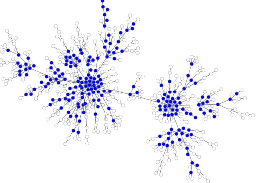
Figure 1.1: The evolution of a preferential attachment graph with change point atγ = 0.4.
(a) Evolution from t= 0.0 untilt= 0.4 with α=−0.5.
Theorem 3.2.1. Fix some parameter set for the change point modelθ= (α, β, γ)andk >1. There exists an integer-valued random variable Dθ such that as n → ∞, the proportion of vertices in the graph with degree k :=Nn(k)/n satisfies
Nn(k) n
P
−→P(Dθ =k), as n→ ∞
However, there exist constants 0< c < c0 such that for all k >1
c
kα+2 6P(Dθ >k)6 c0
kα+2. (1.1)
Notably, the scaling in equation 1.1 does not involve either β or γ. So no matter how big the jump between α and β is, and no matter how early the change point γ occurs, the limiting power-law scaling still only depends on the initial parameter value α. In Chapter 3 we will develop the correct continuous-time branching process framework which will lay bare why this is.
The second thrust of our analysis focuses on trying to answer question (2). How can we best estimate the change point γ?
Our proposal is based on counting leaf nodes. We think this approach is not just elegant, but also potentially extensible to non-preferential-attachment-like networks because it does not explicitly employ the likelihood function for preferential attachment. The rationale is as follows: since the attachment parameter directly affects the chance that new vertices attach to leaves (see Figure 1.1), one ought to be able to feel the effect of the change point through this statistic.
The basic idea behind our estimator is to scan through all time points t in the history of the graph and calculate the difference between:
Then, it makes sense to estimate the change point ˆγ to be the argmax of this function. Actually, we’ll need to scale the difference first—the precise scaling tells us a lot about the unique nature of this change point problem—but we defer a deeper discussion about this point to Subsection 3.3.2 (see Figure 3.2 for an example of Dn(t)).
Dn(t) := (1−t)|th(n)
−h(tn)|, t∈[ε,1] (1.4)
Here’s a walkthrough of how we will prove this estimator is consistent. It turns out that we can calculate what the limitD(t) of this function should be quite easily: it’s constant up to time t=γ, and then decreases smoothly towards 0, which it achieves at t = 1. Therefore if we can just consistently estimate the point at which it starts decreasing, then we are done.
To do this we will need to understand the order of the fluctuations ofDn(t) aroundD(t). We accomplish this via a functional central limit theorem for the proportion of leaves. Let
ˆ
Nn(1, t) be the number of leaves in the graph of size n at time t ∈[0,1]. Then: Theorem 3.2.3. Let p(∞)
t be a function in t describing the limiting proportion (as n → ∞) of leaves in the with-change point graph. Consider the process of re-centered and normalized number of leaves
Gn(t) := ˆ
Nn(1, t)−ntp
(∞)
t √
n , 06t61, (1.5)
with linear interpolation between time points. Then as n→ ∞, Gn
w
−→Gwhere G is a tight Gaussian process on [0,1] and −→w denotes weak convergence on D[0,1] equipped with the usual Skorohod metric.
It follows therefore:
Lemma 3.4.28. Fix ε >0. Then
sup t∈[ε,1]
|Dn(t)−D(t)|=OP
1 √ n
ˆ
γn:= max{t :t ∈ Mn}. (1.6)
Where the setMnis the collection of pointstfor which the corresponding function value Dn(t) is within logn/
√
n of the maximum of the function:
Mn:=
t∈[ε,1] :|Dn(t)−max
t∈[ε,1]Dn(t)|6
logn √
n
(1.7)
Then it follows finally that
Theorem 3.2.4. Assume that the change point γ > ε. Then γˆ is consistent and, in fact,
|ˆγn−γ|=OP
logn √
n
(1.8)
In Chapter 4 we use simulations to examine the performance of this estimator and also to build some more intuition about how it behaves and how it might be extended to other settings. In addition we take the philosophy of looking at functions of the graph history and run with it on two real-world temporal networks to see what lessons we might take from it for future work.
1.1 1.1.2. Decreasing cascades and thinned branching processes
Question: Is a simple, discrete-time branching process model enough to capture the real-world behavior of information cascades?
The next object of study in this thesis is the cascade. A cascade can mean a lot of different things depending on the context. Loosely, a cascade is a process occurring on a graph which spreads across vertices in a way such that affected vertices trigger neighboring vertices in some way in either continuous or discrete time.
Twit-messages to other users who follow them (the user’s “followers”). When a follower receives a tweet, they can either read it passively or choose to pass it on to their followers (“retweet-ing”). And clearly, if an original tweet is interesting enough, then it can trigger a large cascade flowing across the entire Twitter social network.
Generally, we refer to these large cascades as viral. And lately, empirical studies have revealed an interesting of viral cascades: they do not all look the same. Empirical studies have shown that viral cascades can have different shapes, from a very wide but shallow tree sometimes called abroadcast, to a very narrow but deep chain of retweets.
As it turns out, conventional branching process theory does not allow for some of the pos-sibilities. Our goal in this chapter is to take the first step towards achieving these differently-shaped viral cascades using as parsimonious a branching process model as possible.
The cascade we want to model in this chapter is a simple discrete-time models which we call thedecreasing cascade model, chosen because of how closely it mimics sharing dynamics on modern social networks:
Definition 1.1.1. The decreasing cascade
Let G be a graph with vertex set V. A decreasing cascade explores G in discrete time through a set of active nodes, tracing a tree structure in the following way.
Let {pn}n>1 be a decreasing sequence of probabilities.
1. At time 1, start with one infected node.
2. At timen, active nodes infect their unexplored neighbors independently with probability pn. In other words, vertices adjacent to currently-infected nodes become infected with probability pn.
3. Once a node is finished infecting its neighbors or has failed to become infected, it cannot infect any more nodes.
5. Repeat until the cascade dies out or reaches the entire graph.
As it turns out, if we care only about tracking the number of infected nodes in each discrete-time step of such a cascade, then we can re-imagine the decreasing cascade as a sort of two-step branching process. An individual in the process (infected vertex) has a certain number of offspring (the number of neighbors of the vertex) which are then “thinned” binomially to produce their final contribution to the next generation (the number ofinfected neighbors of the vertex).
Definition 1.1.2. The thinned branching process
Let {pn}n>1 be a decreasing sequence of probabilities and let us start with 1 individual in
the system at time 1.
At time n, each individual X gives birth independently to a random number of offspring W, which is distributed according to some offspring distribution F (common to all time steps).
Then, perform Binomial thinning on the offspring by letting only Y ∼Binomial(W, pn) survive until the next generation. Repeat indefinitely or until extinction of the process.
Since many real-world networks have power law degree distributions, we will constrict ourselves to the case where the decreasing cascade is flowing on a scale-free network with degree distribution tail exponent ∈ (1,2)2. It turns out that because of size-biasing, this
is equivalent to setting the offspring distribution F to a power-law distribution with tail exponent ∈ (0,1), implying that the number of infected individuals in each generation is a random variable with infinite mean.
This takes us into uncharted territory. There has been plenty of research into infinite mean Galton-Watson processes and plenty of research into inhomogeneous branching pro-cesses with finite mean.
We contribute one basic result to the literature, which is:
Theorem 5.3.3. Suppose that F is a probability distribution satisfying
1−F(x)∼ C
xα, α∈(0,1) (1.9)
Then a branching process with binomial thinning of such an offspring distribution extin-guishes with probability 1 if and only if the thinning probabilities {pn}n>1 satisfy
− n
X
k=1
(1/α)−klogpk → ∞ as n→ ∞
CHAPTER 2
Background and literature
2.1 2.1. The growth of branching populations
Let us imagine objects that can generate additional objects of the same kind; they may be men or cats reproducing by familiar biological methods, or neutrons in a chain reaction. An initial set of objects, which we call the 0-th generation, have children that are called the first generation; their children are the second generation, and so on. The process is affected by chance events.
-T.E. Harris, The Theory of Branching Processes
The findings in this thesis are actually just glorified studies of very simple branching pro-cesses. Therefore, a thorough understanding of our new results requires a familiarity with some foundational results.
In particular, we will rely heavily on results describing the growth of supercritical pro-cesses—i.e. processes which have some probability of surviving forever. Let us take a short refresher course through the literature on this topic.
2.1 2.1.1. The Dummies’ guide to the Kesten-Stigum theorem
The building block of all branching process theory is the Galton-Watson process.
Let P denote the probability measure of the process. The probability distribution of Z1 is prescribed by putting P(Z1 = k) = pk, for k = 0,1, . . . with Pkpk = 1 where pk is interpreted as the probability that an object existing in the nth generation hask children in the (n+ 1)th generation.
If the process adheres to the following two assumptions,
1. Homogeneity: pk does not depend on the generation number n
2. Independence: All individuals beget offspring independently of each other
then it is aGalton-Watson branching process (“GWBP”) with offspring distribution P. The most basic result in GWBP theory tells us that survival of the family line of Z0 depends
critically on µ, the mean of the offspring distributionP.
Theorem 2.1.1. If µ61, thenP(∃n :Zn= 0) = 1except for the degenerate case ofp1 = 1.
Otherwise when µ >1, P(∃n :Zn= 0)<1.
When the process is guaranteed to die out, we say it iscritical or subcritical, depending on whether µ= 1 or µ <1 respectively. When the process may survive indefinitely, which happens when µ > 1, we say it is supercritical. All in all, the extinction result is not very surprising. It says that if each individual in the system has at most one child on average, then the family line will eventually die out. Most people can believe this.
Where it starts to get interesting is in the analysis of the growth rate of GWBPs. First off, branching processes do not stay stable—they either go the way of the Dodo, or they go the way of Homo sapiens:
Theorem 2.1.2. For any (non-degenerate) regime, P(limZn= 0) +P(limZn =∞) = 1.
But then after that, precise long-run growth analysis depends sensitively on which regime we are in. So just how does one begin to quantify the growth rate of{Zn}n>0, a sequence of
{µn}
n>0 works pretty well, because at least when µ <∞, the sequence {Mn}n>0 defined by
Mn:= Zn
µn, n >0 (2.1)
has EMn = 1 for alln, so that, at least in expectation,µn matches Zn.
But this is not the end of the story. {Mn}n>0 is a non-negative martingale adapted to
the filtration generated by {Zn}n>0, so by the martingale convergence theorem it converges
almost surely to an a.s. finite limit M as n → ∞. Surely, if µn truly measures the rate of increase of the GWBP then we will have EM = 1 as well.
Surprisingly, this is not exactly the case. Indeed, ifµ61, then the GWBP is guaranteed to extinguish and M = 0 a.s. Therefore EMn 6→ EM. But what about the supercritical regime?
It turns out that whether or notµn describes the growth rate ofZ
n in the limit depends on whether the offspring distribution satisfies an XlogX integrability condition. This is the content of the Kesten-Stigum theorem:
Theorem (Kesten-Stigum). Let X stand for a random variable with the offspring distri-bution P. The following are equivalent:
1. E(M) = 1
2. E(Xlog+X)<∞
3. P(M >0)>0
Additionally, we would like to draw the reader’s attention to condition (3) in the above theorem. By the martingale convergence theorem we know that M < ∞ a.s., so that the scalingµncannot fail by being tooslow. What this seems to suggest, then, is that the scaling µn can sometimes be “too fast” and overwhelm Zn, forcing M = 0. But actually1:
Corollary 2.1.3.
P(M = 0|Zn → ∞) = 0
So on the set of non-extinction, Zn ∼ M µn and the different points inside the set {0< M <∞}describe multiplicative ”shifts” of the more-or-less parallel growth of Zn and µn.
To summarize, branching processes are sensitive. They either become so large as to grow indefinitely, or they die out. And in the case with endless growth, there is a very precise rate of growth which is “correct,” and even then we require special conditions on the branching process to achieve it. In the second part of this thesis, we shall try to derive similar conditions on a similar, but wilder type of branching process.
For a concise summary of the main results in the study of the limiting behavior of GWBPs, we direct the interested reader to [76].
2.1 2.1.2. Inhomogeneous and infinite-mean processes
We just showed a conventional martingale analysis of the GWBP. But there is another line of attack to branching process theory using probability generating functions.
Returning to the notation of the previous subsection, the probability generating function (or pgf) of a probability distributionP={pk}k>0 supported on Z+, is
f(s) := ∞
X
k=0 pksk
The beauty of pgfs is that there are a couple different ways of looking at them. For one, pgfs are power series with coefficients in [0,1], so all the usual theorems apply. Secondly, if X ∼P then f(s) = E(sX). Immediate from these observations are results like
1. f(s) is continuous, and specifically continuous from the left ats = 1. 2. f0(s) =P
ksk−1p
3. µ=EX =f0(1)
But also, pgfs are especially relevant with respect to branching processes because we can compose individual offspring distribution pgfs to get pgfs of total population sizes:
Theorem 2.1.4. Let f denote the pgf of the offspring distribution in a GWBP. Also let fn:=E(sZn) denote the pgf of the distribution of Zn. Then
fn+1(s) = f(fn(s))
This gives us an easy way to analyze distributions of future generations of the process. And this can be just as useful as the martingale analysis when examining the behavior of the process in the limit. For example, the extinction theorem 2.1.1 is usually proved using pgfs and, as a side benefit, often make explicit calculations easy:
Theorem 2.1.5. For a supercritical GWBP, the probability of extinction is a solution to the fixed point equation f(s) = s.
Proof. Write Q:={∃n :Zn= 0} for the extinction event so that P(Q) is the probability of extinction. Also let Qn :={Zn= 0}.
Clearly, Qn ⊂ Qn+1 and so P(Qn) ↑ P(Q) as n → ∞. But also, P(Qn) = fn(0). Therefore by Theorem 2.1.4, fn+1(0) = f(fn(0)) which means that P(Qn+1) = f(P(Qn)).
Then since f is continuous,
f(P(Q)) = f( lim
n→∞fn(0)) = limn→∞f(fn(0)) = limn→∞fn+1(0) =P(Q)
1. Varying environment: Let the offspring distributions still be deterministic, but vary by generation.
That is, letφndenote the pgf of the offspring distribution for individuals in the (n−1)th generation. If {φn}n>0 is deterministic, then we are in a varying environment.
2. Random environment: Let the offspring distributions be random across generations, but iid (stationary, ergodic).
That is, let {ζn}n>0 be a sequence of iid (stationary, ergodic) random “environmental
variables” in some space Θ, where we associate with each point ζ ∈Θ a pgfφζ. If φζn is the pgf of the offspring distribution for individuals in the (n−1)th generation, then we are in a random environment.
The case of varying environment has been considered since the dawn of branching processes, and a concise summaries of main results can be found in [64] or [51]. In general, because there is no additional randomness in these processes their behavior can be well-understood so long as one can deal with the analysis of the generation functions.
First, varying environment processes behave similarly to GWBP in many ways. For example, a Kesten-Stigum theorem holds for a class of supercritical varying environment processes. Letµj be the mean of the offspring distribution of the jth generation and call the process uniformly supercritical if
n+k−1
Y
j=k
µj >Bcn for some B >0, c >1, and all n, k >0
Theorem 3 from [45]). If the branching process is uniformly supercritical and is dominated in the sense that there exists a random variable X with EX <∞ such that
P(X > x)>P(Xn/µn> x) for all x,
then there exists a sequence of constants cn such that Zn/cn converges to an a.s. finite random variable W with {W = 0}={Zn→0}.
But there are some surprising differences in contrast to GWBPs. We have seen in the discussion of the Kesten-Stigum theorem that, on the set of non-extinction, a supercritical GWBP has essentially only one rate of growth (up to multiplicative shifts ): µn. As shown in the theorem above, this happens to be true for a large class of branching processes in varying environment. But it is not always so. For example, the authors of [77] construct a branching process in varying environment which is supercritical and grows like 2n on one part of the sample space and mn with m > 4 on another part, both with positive measure. We shall discuss these points further later on in the thesis.
The case of random environment was first introduced in [100] where the sequence{ζn}n>0
was taken to be iid. Their results were later extended to any stationary, ergodic sequence in [8] and [7] where extinction criteria and limit theorems for the process Zn were developed.
The main takeaway from these papers is basically that under some reasonable conditions on{ζn}n>0, we can see the same usual behavior of the ordinary GWBP, with slight obvious
modifications. For the sake of brevity we leave the specifics to the reference.
Theorem 1 from [7]. Under some mild assumptions about the environmental process {ζn}n>0 including an XlogX+ condition, essentially the same results as in the
Kesten-Stigum theorem for Galton-Watson processes apply.
offspring distributions are not taken to be varying, but have infinite mean. While technically these are just supercritical GWBPs, the conditions of the Kesten-Stigum theorem are not at all satisfied, so the limiting behavior is markedly different.
In [94], the authors adapt techniques from the study of finite-mean supercritical branch-ing processes in [95] and [58] to characterize infinite-mean branchbranch-ing processes as either regular orirregular depending on their limiting growth behavior.
Recall from the Kesten-Stigum theorem that, for finite-mean processes, the probability that the martingale limit limn→∞Zn/µn = M is not zero is positive if and only if the Xlog+X condition is satisfied. Therefore in the infinite-mean realm, we say a process is regular if for any sequence of positive constants {cn}n>0 for which limZn/cn a.s. exists, P(limZn/cn= 0 or ∞) = 1.
However, just like how branching processes in varying environment surprisingly can display growth at two different rates, infinite-mean branching processes display interesting exceptions to the finite-mean behavior.
Theorem [94]. There exist infinite-mean Galton-Watson processes such that for some positive deterministic sequence {cn}n>0, the martingale limit M := limn→∞Zn/cn has P(M >0)>0.
Call these theirregular processes. In [94], it is also shown that for all regular processes there exists a slowly-varying functionU(·) such thatU(Zn)/enconverges to a non-degenerate limit. In Chapter 5 we take the first step towards investigating these behaviors for a new, related type of branching process.
2.1 2.1.3. Continuous time branching processes
Say that in a branching process we now want to keep track of the birth, death, and repro-duction times of each individual. Enter the continuous time branching process.
we have a GWBP. If they vary by generation, then we have a branching process in either a varying or random environment.
A continuous time branching process requires a bit more definition. In the most general form, we start by associating with every individual x in the system two processes:
1. λx (the life-length of x): a (possibly infinite) non-negative random variable.
2. ξx: (the reproduction process of x): a point process on N(R+), the space of integer or infinite-valued positive measures on R+ that are finite on bounded sets.2
It turns out that carefully defining these two processes allows us to subsume almost every other classical branching process. We will not dive deeper into the probabilistic setup here. Instead, let us build up some intuition.
One can think of ξx as tracing out the “timeline” of births of the individual x over the infinite time horizon, starting at the time of x’s own birth3. This also means that in order to come into agreement with the physical reality that most things in the universe cannot reproduce after they cease to exist, we will enforce the assumption that the probability that ξx puts any mass after λx is zero, or:
P(ξx((λx,∞)) = 0) = 1 (2.2)
Unless otherwise specified, all following statements will be conditional on no children after death. In general, note that,
1. These processes are homogeneous in the sense that we generally assume the pairs (λx, ξx) to be iid across individuals say with probability distribution Q, a measure on
2We will adhere to the usual point process notation that, for an interval A on the real line, ξ(A) = the
number of points insideA.
3In some places theξ
xprocess is indexed relative to absolute time, so that time 0 represents the start of the
entire branching process. In that case, ifσxrepresents the birth time of xthenξ([0, σx)) = 0. For ease of
the space (R+ × N(
R+)). But they are quite inhomogeneous in the sense that the reproduction ξx within each individual’s lifetime is generally not uniform.
2. Any general branching process can be easily collapsed into the classic discrete-time picture by ignoring λx and recording only ξx([0, λx]) instead of all ofξx.
Aside from this basic assumption though, there are a plethora of possible models to investi-gate.
Example 2.1.6. (Bellman-Harris processes)
A Bellman-Harris process is a continuous-time branching process where an individual’s lifespan and the number of children they bear over their lifetime are independent.
That is, if for each individual x, λx is independent of ξx, then the branching process is a Bellman-Harris process.
Example 2.1.7. (Splitting processes)
A process where individuals are replaced by their offspring, in effect “splitting” into a certain number of other individuals, is called a splitting process. In other words, individuals cannot give birth more than once.
That is, if ξx gives mass to only one random point ν, then the branching process is a splitting process.
If further we haveP(ξx({λx}) = 2) = 1 then each individual always gives birth to exactly 2 offspring—a binary splitting process.
The most important example for the purposes of this dissertation is the Yule process: Example 2.1.8. (Yule processes4)
A process starting with one individual where all individuals live forever and give birth at a unit per-capita rate is a rate-1 Yule process or pure birth process.
4The Yule process dates back to 1925 [114] when it was first used to describe the distribution of the number
That is, if for all individuals x, λx = ∞ and ξx is a rate-1 Poisson process, then the branching process is a rate-1 Yule process. If ξx is a rate-α Poisson process, then the branch-ing process is a rate-α Yule process.
To describe the extinction and growth rate of such branching processes, it will be useful to distill the reproduction point processξx down into a function:
Definition 2.1.9. The reproduction functionof a branching process driven by the life-length and reproduction process (λ, ξ) is
µ(t) = Eξ([0, t]]
so that µ(0) represents the expected number of offspring born instantly, and µ(∞) represents the expected number of offspring born over an individual’s entire lifetime.
Since µ(∞) in the continuous-time case is the analogue of µ, the expected number of offspring in the discrete-time case, it’s unsurprising that continuous-time branching processes follow a similar criticality classification as in the discrete case according to µ(∞).
We say a continuous-time branching process is subcritical, critical, or supercritical ac-cording to whetherµ(∞)<1,= 1, or >1 respectively. As it turns out, the growth behavior of such processes is still roughly the same as in the discrete case. To state the results rigorously, we need just a bit more notation:
z(t) := the number of individuals alive at time t
za(t) := the number of individuals alive at time t who are younger than a
Obviously, if a > t then za(t) =z(t).
Recall that in the case of GWBPs (under appropriate moment conditions), the martin-gale Mn =Zn/µn tells us that,
1. When µ <1, EZn→0 2. When µ= 1, EZn→1 3. When µ >1, EZn=µn
The same trichotomy persists in continuous time. However, the precise rate of growth in the supercritical, continuous case will depend not only on the total number of offspring µ(∞) this time, but on the whole timeline of births µthrough a special parameter α:
Definition 2.1.10. If it exists5, the Malthusian rate of growth of a continuous-time branch-ing process with reproduction function µ is the unique solution α to the equation
Z ∞
0
e−αtµ(dt) =
Z ∞
0
αe−αtµ(t)dt= 1
Where the first equality follows from Fubini’s theorem. α is positive, zero, or negative de-pending on whether µ(∞) is <1,= 1, or >1.
One can think of the integrand e−αt as the continuous-time analogue of the normalizing sequence µn from the supercritical GWBP. And we see that it plays a similar role in the asymptotic analysis.
Theorem 6.3.3 from [65]. Under some reasonable conditions on µ,
1. If µ(∞)<1, then
Ez(t)→0 as t→ ∞
2. If µ(∞) = 1, then for all 06a <∞,
Eza(t)→C1 as t→ ∞
5In certain edge cases it does not, for example ifµ(0)>1 then we may have
where C1 depends only on a, λ, and ξ.
3. If µ(∞)>1, then for all 06a <∞,
Eza(t)∼eαtC2
where α is the Malthusian rate of growth and C2 depends only on α, a, λ, and ξ.
Let us see by example what this can tell us. Example 2.1.11. (Growth of a rate-ν Yule process)
The rate-ν Yule process’s reproduction is driven by a rate-ν Poisson point process so the reproduction function is given by µ(t) =νt. Therefore the Malthusian parameter is solved by
1 =
Z ∞
0
αe−αtνtdt=να
Z ∞
0
te−αtdt=να
1 α2
Yielding α = ν. Therefore since ν > 0, the Yule process is supercritical and the population size grows roughly at rate eνt as t→ ∞.
In Chapter 3, we conduct essentially the same analysis, except instead of a Yule process driven by Poisson point processes, we will study a branching process driven by Yule processes viewed as a point process. We will also make use of stronger limit theorems giving us a.s. and L1 convergence of z(t).
2.2 2.2. Networks
2.2 2.2.1. Scale-free networks
for appropriate values ofk. In reality, many real-world networks deviate from this prescrip-tion due to finite-size effects. For example, it is common for many social networks to exhibit an exponential cutoff at some large k, see for example [35]. For simplicity in what follows we ignore these effects.
The timing of the surge coincides with the fact that technological advances have allowed us to examine the properties of massive networks such as the Internet and citation networks and discover that many of these have power law degree distributions. Indeed the recent resurgence in the study of scale-free networks can be traced back to Barabasi’s empirical discovery that the network of the internet has a power law indegree distribution with α = 2.1±0.1 [4]. Since then many other networks have been shown to exhibit power law degree distributions, spanning a range from networks in social science to the humanities. There are too many examples to name here—see [43] for a more exhaustive discussion—but one particular class of networks is worth mentioning for later reference.
It is known that the social network Twitter exhibits much stronger scale-free character-istics than other popular social networks such as Facebook ([71], [105]). On Twitter, the majority of interactions between users are passive in nature—once a user A “follows” another user B, user A will see all content that user B posts onto the network. This is similar to Facebook, except with one crucial difference. On Facebook a user mustrequest a connection (“send a friend request to”) with another user and wait for that other user to approve the friendship connection before they are connected. On Twitter, the vast majority of users can be followed by any user without a need for the request to be approved. This allows for much higher outdegree distributions which appear closer to a true power law, as shown in [71] and [102], among others.
shown that preferential attachment graphs withm >2 have diameter that instead scale like logn/log logn. These results have implications for a wide-range of graph problems, from routing [19] to epidemics and information diffusion [86] (also discussed later).
The study of scale-free graphs has only accelerated recently, but the notion itself is actu-ally quite old. The Erdos-Renyi random graph model was introduced in 1959. Just 6 years later in [88], Price noticed that citation networks exhibit a power law degree distribution. A decade or so later in [89], Price posited the so-calledcumulative advantage mechanism which generates a network with power law degree distribution according to a simple rich-get-richer scheme: new vertices attach to an existing vertex with probability proportional to the degree of the existing vertex. Over a decade later, this was re-discovered by Barabasi in [10] and is now more commonly known as the preferential attachment (PA) mechanism.
This model has become one of the standard workhorses in the complex networks com-munity. At this point it is impossible to compile a representative list of references, we will try to give an overview, restricting ourselves as far as possible to papers close in spirit to this project; see [103] where it was introduced in the combinatorics community, [10] for bringing this model to the attention of the networks community, [82],[43] for survey level treatments of a wide array of models, [23] for the first rigorous results on the asymptotic degree distri-bution, and [36], [21], [93], and [46] and the references therein for more general models and results.
2.2 2.2.2. Preferential attachment
The canonical way of growing scale-free networks is preferential attachment, and this is the model with which we concern ourselves in the first part of this proposal. There are several variants of the preferential attachment model, but all share the same basic mechanism:
1. Start with two nodes with m edges between them.6
2. At time n add one vertex with m edges to the existing graph in the following way.
(a) Link the first edge to an existing vertex v with probability proportional to some function f(Dn−1(v)) where Dn(v) is the degree of v at time n.
(b) Update the degrees of all vertices in the graph (c) Repeat (a) and (b) until all m edges are connected.
At time n there will be 2 +n vertices and total degree 2mn. For the rest of this section we will concern ourselves with the case of trees m= 1, both for simplicity of exposition and because the general case can always be reduced to the case of trees.
The variations in the model concern the function f(·). In the original Barabasi-Albert formulation, f(Dn−1(v)) =Dn−1(v), i.e. the probability of connecting to an existing vertex v is proportional to the degree of v. The simplest generalization of this model is sometimes referred to as linear preferential attachment in which
f(Dn−1(v)) =Dn−1(v) +α, α>−1
Since this model encompasses the original (the special case α = 0), we will sometimes let preferential attachment mean linear preferential attachment. Note that as α → ∞, we have the so-called uniform attachment scheme in which new edges attach to existing vertices uniformly at random.
The preferential attachment model has become one of the standard workhorses in the complex networks community, based in part on the fact that it exhibits the power law/heavy tailed degree distribution observed in an array of real world systems. As the literature on preferential attachment is large and very broad, we focus on work that is close in spirit to the
6Some formulations of the model begin with a single node and m self-loops. In both cases the limiting
work in this thesis. The preferential attachment model was introduced in the combinatorics community in [103] and was brought to the attention of the networks community in [10]. The papers [82] and [43] give survey-level treatments of a wide array of related models, while [23] gives the first rigorous results on the asymptotic degree distribution. More general models and results can be found in [36], [21], [93], [46], and the references therein.
For all its simplicity, the PA mechanism can be viewed in a deeper light through a continuous-time heuristic which turns out to be very useful. Essentially, the PA process is a type of Polya urn process, which can be embedded into a natural continuous-time process related to the Yule process.
A rate-γ Yule process {Yγ(t) : t >0} is a continuous-time process which starts at time 0 with 1 individual where individuals in the system survive forever and give birth to new individuals independently of other individuals and at rate γ (i.e. the waiting time between births is∼exp(γ)). When γ = 1 we shall call this point process the standard Yule process.
To foreshadow the connection with our work in the second chapter, let us flesh out this point process explicitly. Suppose that {e(k)}k>1 is a sequence of independent exponential
random variables with e(k) ∼ exp(k). If we view these as inter-arrival times of a point process P0 onR+, i.e.
L(m) =e(1) +. . .+e(m), P0 := (L(1), L(2), . . .)
then P0 is exactly a standard Yule process.
If we initiate two rate-α Yule processesY1
α(t), Yα2(t) at the same time, then the numbers of individuals in the processes evolves exactly like a 2-color Polya urn starting with one ball of each color. More precisely let Ni
α(t) denote the number of points in Yαi(t) at time t and write Y(t) = (Nα1(t), Nα2(t)). If X(n) = (X1(n), X2(n)) is the Polya urn process at step n
mentioned above, then
To see this, note that at any fixed time t0 the probability that Yα1 increases by 1 before Y2
α does is the probability that the minimum of Yα1(t0) iid exp(α) random variables is less
than the minimum of Y2
α(t0) iid exp(α) random variables, which by the properties of the
exponential distribution is proportional to Y1
α(t0)/(Yα1(t0) +Yα2(t0)). This is exactly the
probability that a ball of the first color is picked next in a 2-color Polya urn with Y1
α(t0)
balls of the first color and Yα2(t0) balls of the second color.
To make the connection to the preferential attachment model, recall that we start with two vertices (labelled 1 and 2) linked with an edge and suppose we haveα = 0. Clearly the model evolves as the number of balls in a 2-color Polya urn, where the colors correspond to the family lines of either vertex 1 or vertex 2. This simple model is of limited value, but a simple modification yields the bedrock of all later analyses.
First, we need to set up a small variation on the standard Yule process. Let {Eα(k) :k >1} be a sequence of independent exponential random variables as before ex-cept now suppose Eα(k) has ratek+αrather than k. Viewing the above as the inter-arrival times of a point process Pα on R+ and setting Lα(m) =Eα(1) +· · ·+Eα(m) for m >1 as
before, define the point process
Pα := (Lα(1), Lα(2), . . .). (2.3)
Note thatP0 is exactly a rate-1 (or standard) Yule process. For fixed t>0, write Nα(t) for the number of points in Pα which fall in the interval [0, t]. This process will drive our key branching process:
Definition 2.2.2 (Continuous time branching process). Fix α >0. We let{BPα(t) :t>0} be a continuous-time branching process driven by the point process Pα in (3.4). More pre-cisely:
(a) At time t = 0 we start with one individual called the rootρ which has offspring distribu-tion Pρ
α d
(b) Every new vertex v that is born into the system is given it’s own offspring point process Pv
α d
=Pα, independent across vertices.
Fort>0, we will view BPα(t) as a (random) tree representing the genealogical relation-ships between all individuals in the population present at time t. Now set:
τn := inf{t :|BP(t)|=n}
WritingTn for the preferential attachment tree grown with parameterαuntil sizen, we have
BP(τn) =d Tn, viewed as random rooted trees. But more than that, we have that the two processes of growing random trees have the same distribution namely
{BP(τn) :n >1}
d
={Tn:n >1}.
Thus we have extended the simple idea of an urn process embedded in Yule processes to describe, in continuous time, the evolution of the entire preferential attachment tree. This is the fundamental idea behind our entire analysis of the changepoint regime. Later on we shall derive the Malthusian rate of growth for this process on the way to other limit theorems as well.
2.2 2.2.3. Changepoint detection on networks
The general changepoint detection problem has a vast history owing to its obvious importance in applications such as quality control and reliability of industrial processes, in particular quick detection of process failure in production, as well as fields such as signal processing (e.g. biomedical data including neuronal spike data and seismic data), automatic segmentation of signals into stationary segments via identification of change points etc. An exhaustive overview of the classical literature can be found in [11].
detection” on networks is actually the study of detecting anomalies from what is predicted by the model, without a natural temporal aspect. Indeed there has been a significant amount of work on developing techniques to detect anomalous subgraphs and motifswithinnetworks, see e.g. [48, 2, 83, 90, 57, 96], for a wide-ranging survey see [29]. This also includes anomalous edge detection via link prediction algorithms [61].
There has been less work done with temporal (time-varying) networks. Much of the work in this area is centered along quantifying anomalies in a sequence ofdeterministic sequence of graphs, see for example [101], [83], [1]. The changepoint problem on a sequence of a graphs (e.g. across time) with a probabilistic model underneath is less explored and we discuss it here.
Classical changepoint detection is essentially focused on detecting changes in parameters of an independent (or stationary) sequence. This is where network changepoint problems start to diverge from the classical regime. First of all, network data is often far from inde-pendent, especially if the network size is growing as in dynamic models mentioned below. Secondly, the changes we are interested in often go beyond simple shifts in parameters. We may be interested in more complicated concepts such as changes in community structure or more complicated quantities such as the clustering coefficient. All of these present difficulties when appealing to existing theory.
It is convenient to think of generative network models as falling into one of two classes: static models or dynamic models. In static models the network size is fixed, whereas in dynamic models the generative mechanism directly models the growth of the network over time. The ER(n, p) Erdos-Renyi random graph on n vertices is a static model, whereas the P A(1, α) preferential attachment is a common dynamic model. This distinction carries over to changepoint problems on networks in a natural way.
fixed across time. If the networks in the sequence are taken to be independently generated, then adapting classical changepoint concepts is even more straightforward. The simplest way to do this is to convert the graph sequence to a scalar sequence and apply traditional techniques. In [78] the authors consider a sequence of independentER(n, p) graphs in which, after a certain point, a subset of nodes begins to connect to each other with higher probability than to the other nodes in the graph. The bulk of the paper is devoted to selecting a proper test statistic, but the stopping rule for actual changepoint estimation still comes back to Average Run Length (ARL) theory. This also is the approach followed in [79]. Even in cases when the graph sequence cannot be easily reduced to a scalar sequence, independence across a static sequence is easy to analyze. For example [87] purport to develop an “entirely general” changepoint detection method using thegeneralized hierarchical random graph model, but at its core their approach is simply maximum likelihood on a sequence of independent graphs. By and large however, it is unreasonable to assume that from time t to t+ 1 that the entire graph is independently regenerated, especially if the underlying entities represented by the nodes are fixed. Inspired by voting record graphs from the US Congress (i.e. two congressmen are joined with an edge if they voted together on a bill), [113] has proposed a simpleER(n, p) variant with Markov chain dependence for the presence of an edge between a particular pair of vertices, and analyzed the natural changepoint question arising from that chain. These methods depart somewhat from classical changepoint formula, but still confront a relatively simple situation: a sequence of graphs with a fixed number of vertices and underlying generative model, with a well-understood dependence structure across graphs.
depends on the entire existing structure of the graph, so individual placements are neither independent, stationary, nor ergodic. This calls for a completely different approach than in standard univariate changepoint analysis.
2.3 2.3. Cascades
2.3 2.3.1. What is a cascade?
In general, a cascade is a process occurring on a graph which starts at a single node and spreads across vertices in a way such that affected vertices trigger neighboring vertices in some way. In this way, it is distinguished from other interacting models on a graph (Ising model, voter models) where all particles interact with all other particles simultaneously.
But even then, acascade can mean a lot of different things depending on the context. In the economics literature [14], an informational cascade is a process spreading over a group of individuals in which an individual, having observed the actions of those ahead of him, follows the behavior of the preceding individual without regard to his own information. In this sense, a cascade is a sort of herd mentality process. In other contexts, a cascade can refer to a sort of epidemic model where individuals are carriers for a disease and the disease propagates to other individuals according to some mechanism.
To narrow down our discussion to those models relevant to our study, let us first propose a rough classification. Essentially, all cascade models fall into one or more of these three categories, based on how the mechanism for propagation is defined:
1. Agent-based models:
In most of these cases, the graph is implied or de-emphasized, e.g. [14] or [9], but there are exceptions. In [37] for example, the authors investigate agent-based diffusions on the classic Watts-Strogatz small world network.
2. Continuous-time, rate-based models:
These models specify the rate at which a cascade passes from individuals to one an-other, and encompasses most epidemic models such at the SI/SIR/SIS models. In these models, the basic dynamic is that uninfected neighbors of infected nodes (sus-ceptible notes) become infected at a certain rate and then either stay infected forever or recover at certain other rate. The steady-state is then generally studied using a mean-field approach—approximating the random process flowing on the graph using a set of deterministic differential equations.
These types of processes are well studied—variations on the SI/SIR/SIS paradigm are especially ubiquitous, see [42] or [115] for typical examples. Therefore we will not go further into it here besides to direct the reader to [46, 85, 63] for comprehensive analyses and overviews.
3. Discrete-time, probability-based models:
These models directly specify the individual probabilities of transmission between ver-tices and is the tradition within which we study them here.
It is worth noting that there is some degree of overlap between all three of these categories. Almost any model in one of these three categories can be reduced to or put in terms of another, if one tries hard enough.
popular each state is among their peers. But the model can also be analyzed in a probabilistic light—by recursively calculating probabilities for whether vertices n steps away from the source of the cascade become infected. Other models such as [60] explicitly involve a rate of infection and a threshold model.
However, what does generally remain true to each category are the styles of methods used in and results obtained from each one. The model most relevant to us is theindependent cascade model first elucidated in [54]. We quote from [70]:
The cascade starts with an initial set of active vertices and then unfolds in discrete time according to the following rule. When a vertex v becomes active in step t, then it is given a chance to activate each currently inactive neighborw; it succeeds with a probability pv,w—a parameter of the system—independently of the history thus far. (Ifwhas multiple active neighbors, then their attempts are sequenced in an arbitrary order.) If v succeeds, then w becomes an active vertex in step n+ 1; but whether or not v succeeds, it cannot make any further attempts to activatew in subsequent rounds.
Indeed, this model is so simple that it is sometimes referred to in the literature as the “cascade” model (as opposed to “threshold” models). Its simplicity makes it amenable to analysis and, in fact, many studies involving estimation ofpairwise transmission probabilities implicitly study this model. See for example [92, 55]. There is also a long chain of research involving influence maximization using this model, i.e. discovering which set of vertices to activate initially in order to achieve the largest resulting cascade, see [70] or [30] for two representative papers on the general theory—see [110] for an extension targeting the Twitter network.
constant probabilities (i.e. pv,w = somepfor allv, w∈V) can be modelled by some binomial-based branching process. Indeed if a graph is large enough, one would expect a branching process approximation to work quite well in modelling the growth of the cascade. In this thesis our setting will be that of graphs with infinite variance, which, under size-biasing, takes us into the realm of branching processes with varying environment and infinite mean. However, the most attractive feature of this model to us is the fact that the probabilities pv,w can be varied in a simple way. Not only does this reflect one’s intuition about reality, but it also opens the door to the possibility of producing a wide array of cascade behaviors through adjustment of only the probabilities. This general scheme is not new. For example, in [112] the authors propose the closely-related linear influence model which also models an independent cascade process whereby the transmission probability for a given cascade is a linear function of the “influence” of the nodes which the cascade has passed through previously. We find this model both more complicated and less salient for the social networks we model. The independent cascade paradigm is also tackled in [55], where the inferential question of learning the transmission probabilities at each node of the network is undertaken. In neither of these cases is a rigorous probabilistic analysis carried out.
2.3 2.3.2. The shape of viral cascades
So how do cascades look like in reality? Do any of the cascades models mentioned above actually do a good job of modeling them? Thanks to smartphones and social media, we have many examples to mine.