An improved phylogenetic tree comparison method

(1)

Suneel Potiny

A thesis submitted to the faculty of the University of North Carolina at Chapel Hill in partial fulfillment of the requirements for the degree of Master of Science in the Department of Biomedical Engineering

Chapel Hill 2010

(2)

ii Abstract

Suneel Potiny

An improved phylogenetic tree comparison method (Under the direction of Dr. Shawn Gomez)

(3)

iii

List of Tables

Table 1 – Species Character Chart ... 8

(6)

vi

List of Figures

Figure 1 – Rooted and Unrooted Trees ... 3

Figure 2 – Proposed Phylogenetic Tree ... 9

Figure 3 - Reconstruction of character 1 on proposed tree. ... 10

Figure 4 - Reconstruction of character 2 on proposed tree ... 10

Figure 7 – NNI diagram ... 16

Figure 8 – Partition Diagram ... 17

Figure 9 – MAST Diagram ... 19

Figure 10 – Quartet Diagram ... 20

Figure 11 – Updown Diagram ... 22

Figure 12 - Generating Distance Matrices ... 28

Figure 13 - Procrustes with Euclidean Structures ... 30

Figure 14 - MDS-Procrustes distribution for validation dataset ... 32

Figure 15 – Random Search Query ... 34

Figure 16 – Random Search Top Ranker ... 34

Figure 17 – Random Search Top Rank Subtree ... 35

Figure 18 – Random Search Second Ranker ... 35

Figure 19 – Random Search Second Ranker Subtree ... 36

Figure 20 – PAR distribution for initial dataset ... 38

Figure 21 – MAST distribution for initial dataset ... 39

(7)

vii

Figure 23 – Quartet distribution for initial dataset ... 40

Figure 24 – Usim distribution for initial dataset ... 40

Figure 25 – MDS-Procrustes distribution for initial dataset. ... 41

Figure 26 – Exact Match Tree 1... 42

Figure 27 – Exact Match Tree 2... 43

Figure 28 – Par Distribution for second dataset ... 44

Figure 29 – MAST distribution for second dataset ... 44

Figure 30 – NNI distribution for second dataset ... 45

Figure 31 – Quartet distribution for second dataset ... 45

Figure 32 – Updown Distribution for second dataset ... 46

Figure 33 – MDS-Procrustes distribution for second dataset ... 46

Figure 34 – Runtime Comparison ... 50

(8)

Chapter 1 Introduction

1.1 Phylogenetic Trees

(9)

2

can be theorized that two species with similar phylogenetic tree structures would contain genes or proteins that co-evolve with one another, these comparisons can be a useful method for predicting such phenomena and continued work in this area can be informative.

1.2 Types of Phylogenetic Trees

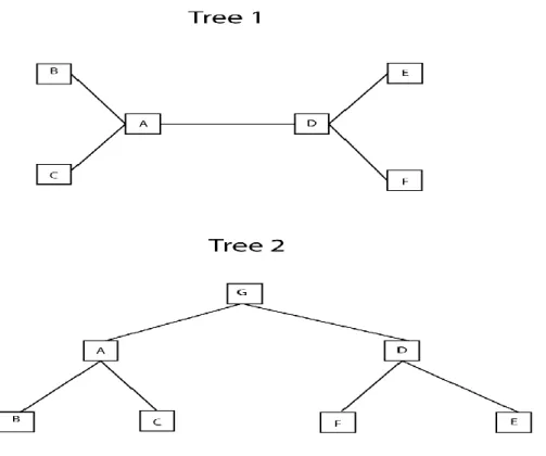
In a phylogenetic tree, each internal node with descendant nodes represents the most recent common ancestor of the descendants. Each node in the tree is called a taxanomic unit and internal nodes are commonly known as Hypothetical Taxonomic Units(HTUs) since they often cannot be directly observed. Phylogenetic trees can either be rooted or unrooted. A rooted tree refers to a tree in which all leaves in a tree share a common ancestry to a “root” sequence or node. An unrooted tree is a tree that makes no inferences about the ancestry of the leaves contained therein and can be useful to visualize related sequences contained in a particular organism(despite the ancestry being unknown). Figure 1 shows both a rooted and an unrooted tree.

(10)

3

Figure 1 – Rooted and Unrooted Trees

Tree 1 shows an unrooted tree. Tree 2 shows the same tree as in Tree 1, except it becomes rooted with a common ancestor (G). It can be seen from this figure that a rooted tree can become unrooted by removing the root node (ie removing Node G from Tree 2 to transform it into Tree 1), however the converse is not true.

Additionally, both rooted and unrooted trees can be either bi-furcating or multi-furcating. A bifurcating tree is a tree in which each internal node has exactly two immediate decendants. A multi-furcating tree can have nodes with more than two descendants. Trees can also be either labeled or unlabeled. A labeled tree has values assigned to its nodes, while unlabeled trees only define a topology of relationships between sequences/events without containing information about the nodes themselves.

(11)

4

divergence between two sequences or species. Often times it is useful to think of this as a measure of time in which the node was changed from its ancestor. The ability to obtain this information can be difficult and while there are existing hypotheses (such as the molecular clock that uses fossil constraints and rates of molecular change to compute this time), they often contain a great deal of error and cannot always be used with much confidence in a scientific study. However, if this information exists, it can obviously be extremely useful in deducing similarities among taxa between species, as it gives more definition to the topology of a particular tree.

One commonly used technique for obtaining these distance measures is by looking at the similarity between two or more biological sequences across species (generally DNA, RNA, or protein sequence data obtained for a particular set of species). In order for this measure to generate a biologically relevant tree, the sequences being analyzed should be homologs (known to derive from a common ancestor). There are many models available to analyze the similarity between two homologous sequences and determine an evolutionary distance between the sequences. One such model is the Kimura substitution model. This DNA substitution model assumes that changes between the two base types (pyrimidines and purines) occur at different rates than changes within the base types (thus changes from A->G and T->C occur at one rate and changes across base types occur at a different rate). To illustrate this process, we will look at the following two homologous, aligned input DNA sequences from two different species (1 and 2):

1 - AGAATAGTTAG

2 - CGATGA –T – AG

(12)

5

A G T C

A 0 1 0.5 0.5

G 1 0 0.5 0.5

T 0.5 0.5 0 1 C 0.5 0.5 1 0

We will also assign a gap penalty of 2 in this example (to correspond to a deletion event in a sequence). Thus, based on the above given information, for this particular example we get the following output:

S(A,C) + S(G,G) + S(A,A) + S(A,T) + S(T,G) + S(A,A) + (gap penalty) + S(T,T) + (gap penalty) + S(A,A) + S(G,G) = (0.5) + (0) + (0) + (0.5) + (0.5) + (0) + (2) + (0) + (2) + (0) + (0) = 4.5

So, the calculated evolutionary distance between the sample sequences would be 4.5. In this form of analysis, the greater the evolutionary distance, the longer the time it would take for one

sequence to evolve into the other.

The above example was a simple pairwise distance measurement, but of greater significance to studies on phylogenetic trees are alignments of multiple sequences (MSAs). There are several methods available find the optimal alignments (alignments that minimize the distance measure) between multiple sequences, including ClustalW and T-coffee. These

(13)

6

1.3 Construction of Phylogenetic Trees

As previously stated, the development of sequencing technology has benefited the study of evolutionary relationships among organisms. The data from a sequence alignment (along with other types of data) is often used in phylogenetic tree reconstruction. Construction of

phylogenetic trees is generally based on cladistics (the systematic classification of organisms on the basis of shared characteristics deriving from a common ancestor). The different construction methods can loosely be categorized into three different types: Distance-based methods, character based methods, and probabilistic methods.

Distance-matrix methods (such as Neighbor-Joining, Fitch-Margoliash, or Unweighted Pair Group Method (UPGMA)) generally require a multiple sequence alignment (MSA) as input. The example in the previous section briefly illustrated how this distance can be calculated and provided this distance value, evolutionary origin can be inferred. Distance-matrix methods generally function by clustering the nodes together based on the input distance information resulting from a sequence alignment. Due to the complexities of the input into these methods, the algorithms to produce this are computationally complex and consequently heuristic approaches are often used to help simplify the problem.

Character based methods treat differences between the input sequences as discrete characters with each character considered to be in a particular state (e.g. present vs not present). The most common character based method is maximum parsimony. In this approach, a

(14)

7

standard statistical analysis to infer a probability distribution from this data and generate a particular phylogenetic tree.

However, the problem of finding a suitable phylogenetic tree given even a relatively small set of nodes is computationally intensive. This occurs because the number of possible tree structures that can be created from a set of species or sequences greatly increases with the inclusion of each additional unit. Given a set of species, , the following equation defines the number of possible formations of a rooted, bifurcating and unweighted trees:

( )

(1)

This equation can easily be computed to show that the number of possible trees grows greatly with additional nodes (at =1 there is 1 possible tree, at =5 there are 105 possible trees and at

=10 there are 34,459,425 possible trees). Since any unrooted tree can be made a rooted tree simply by omitting the root, it is clear that the number of unrooted trees possible is less than the number of rooted trees. When adding a node to a tree in all possible positions, you would simply add it to each existing branch in the tree. And combining this with the fact that a rooted tree is made unrooted by removal of the root node, we see that the number of possible rooted,

(15)

8

1.4 An Example of Character Based Phylogeny Reconstruction

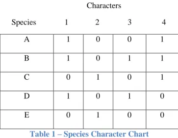
To further illustrate the process by which a tree is constructed, we will look at a simple character based example and use a maximum parsimony approach to partially evaluate the proposed phylogenetic tree’s accuracy (Felsenstein 2003). Table 1 below shows a list of five species and each species’ character state for 4 chosen characters (for simplicity, we will assume that the characters each have two states, 0 and 1).

Characters

Species 1 2 3 4

A 1 0 0 1

B 1 0 1 1

C 0 1 0 1

D 1 0 1 0

E 0 1 0 0

Table 1 – Species Character Chart

Table shows species and the corresponding state for each of 4 different characters.

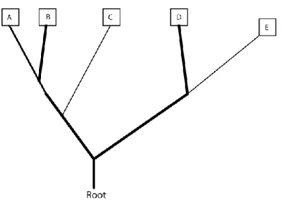
From here, we will generate a random, rooted phylogenetic tree structure with 5 nodes representing each of the species. The tree that we will evaluate here is shown in figure 2.

(16)

9

In figure 3, from the chart we see that species A and B have the same state for character 1, so there is no change of state at the node connecting those two species. The next node is connecting this subtree to species C, which has a state different than that of species’ A and B, so for this tree to be accurate according to the chart, there must be a change of state along the branch connecting the A-B subtree to C (depicted by the bold line, signaling a change in state from 1 to 0). This same convention is used throughout the figures, so the number of changes in state can easily be counted by looking at the number of times the lines go from normal to bold. In these figures, we assume the state of the root is the same as the left side of the tree at the point which it attaches to the root. Thus, if there is a change of state from the left side to the right side of the tree, we show that change of state occurring on the right side of the tree along the branch leading from the root to the D-E subtree.

Figure 2 – Proposed Phylogenetic Tree

(17)

10

Figure 3 - Reconstruction of character 1 on proposed tree.

Character state changes from 1 to 0 along the branch extending from A-B subtree to species C and also from the Root to species E. Two total changes of state.

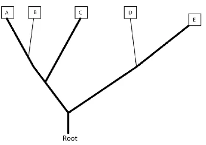
Figure 4 - Reconstruction of character 2 on proposed tree

(18)

11

Changes of state from 0 to 1 occur along the branch leading to species B and the branch leading to species D. 2 total changes of state.

(19)

12

We then compute the total number of state changes across each of the characters (2+2+2+1) to get a total of 7 changes for this particular tree. In a maximum parsimonious approach, this number of changes would be compared to all other possible tree constructions to determine the most desirable tree for the informative characters defined in Table 1.

1.4 Comparison of Phylogenetic Trees

The comparison of these phylogenetic tree structures can be very informative. As stated previously, since the data contained in these trees represents genetic or other biological

similarities across species, much can be explained from analyzing evolutionary trees. With several databases, such as TreeBASE(Sanderson 1994), publicly available for scientists to upload and analyze their own constructed trees with other existing trees, the need for finding a suitable method for comparing these trees is increasing. While many current methods exist, the distance-based method presented in this paper is shown to be useful and in many ways superior to other existing methods analyzed in previous studies.

(20)

13

Also, these comparisons can be useful as a means of analyzing co-evolution between various species or molecules. This is commonly seen in host-parasite relationships. An example of this would be the relationship between the attine ant, the fungi that it cultivates, and the Escovopsis parasite (Currie 2003). It is often assumed that genes and proteins in these types of symbiotic relationships will change together, so that a change in one will correspond to a change in the other as a means of adaptation. Comparing trees for similarity can greatly aid in predicting these events.

Furthermore, outside of the aforementioned biological uses of these methods, comparing trees can be useful in other disciplines as well. Any system that attempts to predict events based on a previous history of input (such as search algorithms which attempt to suggest things to buy or view based on your previous purchases or search criteria) can often times be categorized in tree structures and so comparing them can aid in the predictive abilities of such tools. The goal of this paper is to evaluate a new method and compare it to the already existing methods in hopes that it can be a potentially useful tool for scientists and researchers/developers in these areas of interest.

In the method (referred to as MDS-Procrustes) presented here, we use classical multi-dimensional scaling to represent the distances between nodes within a tree as structures in a high dimensional space and then attempt to fit each tree’s structure together through a Procrustean-related approach to determine the similarity of the two trees. To understand the approach and how it improves in solving the problem of comparing trees from databases, it is important to fully discuss the advantages/disadvantages of existing methods (which will be explained in the

(21)

14

1.5 Existing Comparison Methods

Existing methods for comparing phylogenetic trees can generally be classified into two categories, methods that compare trees based on topological features and distance-based methods. In Choi and Gomez (2009), a similar approach to MDS-Procrustes was compared the

tol-mirrortree approach presented by Pazos and Valencia (2001) in the prediction of protein-protein interaction networks. It was shown there that this technique offered an improvement to some distance based methods and here we will extend that work to show how it also outperforms many of the topological methods in the specific problem of comparing phylogenetic tree structures for similarity. Topological methods generally ignore the distances between tree nodes and instead rely on comparing trees for similarity based on related topological features and relatedness between taxa (Quartet, Partition, Maximum Agreement Subtree, Updown) or on transforming one tree into another (Nearest Neighbor Interchange). While these methods can be useful in certain limited comparisons or in generating groupings among trees, we find that they either do not scale well to comparisons on large data sets of many trees with many different nodes or do not offer the distribution of similarity scores necessary to effectively rank trees by similarity score values.

To fully evaluate the quality of the proposed method, we compared MDS-Procrustes to several existing methods found in the literature by looking at computational time and similarity score distribution. The metrics we compared our method to here are Nearest Neighbor

Interchage (NNI), Partition (PAR), Maximum-agreement subtree (MAST), Quartet, and Updown (USim). These metrics are among the more popular methods found in the literature and have proven to be very useful methods in previous studies (Steel and Penny 1993, Wang 2005). All of these methods are topologically based (as opposed to our distance-based metric) and thus rely on direct relationships among nodes to determine similarity. In the proceeding sections, we discuss and illustrate each of these methods before offering a full analysis of our proposed

(22)

15

1.6 Nearest Neighbor Interchange Metric

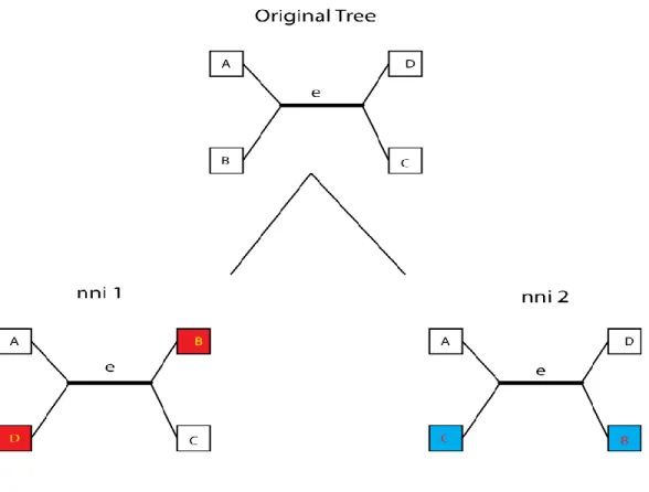
The NNI metric refers to the number of near neighbor interchange operations necessary to transform the query tree into the data tree (we use the term query tree to refer to the tree for which we are searching through a data set of data trees to find a nearest match). It essentially involves the swapping of nodes around a common edge of the query tree until the data tree is fully realized. In a labeled binary tree, the end points of each interior edge will be adjacent to two distinct subtrees. A nearest neighbor interchange simply involves the interchanging of these two subtrees, one adjacent to each endpoint. Figure 7 illustrates this process and shows a tree and the two possible nni operations along a particular interior edge. In the figure, the internal edge e induces two separate subtrees, A-B and D-C. The two possible nearest neighbor interchanges on that edge that would induce different subtrees from that edge involve swapping B and D (to induce subtrees A-D and B-C) or swapping C and B (to induce subtrees A-C and D-B).

A binary subtree with nodes will have -3 interior edges. Conversely it can be

(23)

16

Figure 7 – NNI diagram

Shows the two possible Nearest Neighbor operations along internal edge(e). The

highlighted nodes in the two trees below the original tree shows how the tree transformed in each case by using 1 NNI operation along edge e.

1.7 Partition Metric

(24)

17

they would have no different partitions. Figure 8 shows two trees and details the different Robinson-Foulds partitions that exist between them. In the figure, it is easily seen that the only difference between the trees is that the positions of nodes E and C are transposed. When computing the symmetric difference, we look at the partitions created upon the removal of each internal edge of the tree. When doing that in this example, it is seen that the only times that separate partitions are created occur when the highlighted edges are removed. In tree 1, when we remove the highlighted edge, the partitions created are {(A,B,E),(D,C)}, while in tree 2, removal of the highlighted edge generates the partitions {(A,B,C),(D,E)}. Removal of the other internal edges in either trees leads to the same partitions and thus for these two trees, the symmetric difference is equal to 2.

Figure 8 – Partition Diagram

Shows two trees and the partition distance between them. The highlighted edges show the different edges between the two trees and the partitions that result from a deletion of that edge. The partition distance between these two trees is 2.

(25)

18

moving the root of the tree to a different spot (and leaving all other nodes the same) can lead many different partitions between the two trees, thus indicating that the trees are extremely different, even though they only differ in the placement of one node. Also, the distribution scores that it can provide are limited to the number of branches in a tree and thus it is not able to provide a good enough distribution to be able to effectively rank trees according to similarity.

1.8 Maximum Agreement Subtree(MAST) metric

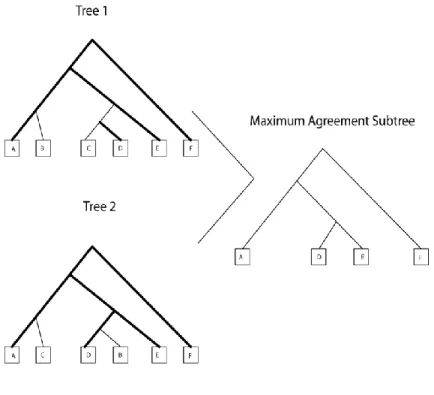
The maximum agreement subtree (MAST) method is another relatively straight-forward topological metric used for comparing two trees. In this method, introduced by Gordon (1979), the objective is to choose a subtree from the query tree for which there is an equivalent match in the data tree. A subtree of a tree T is a tree consisting of a node in T and all of its descendants in

T. The maximum agreement subtree is the subtree with the highest number of nodes from the original tree. The metric used in this paper is equal to the number of leaves removed from the data tree to obtain this maximum agreement subtree. Figure 9 shows two trees and the maximum agreement subtree between them.

(26)

19

Figure 9 – MAST Diagram

Shows two trees and their Maximum Agreement Subtree(MAST). The highlighted branches show the branches that exist in both trees to form the MAST structure.

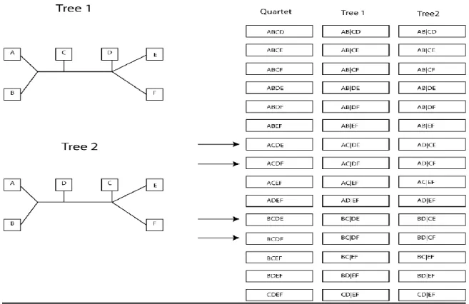
1.9 Quartet Metric

The quartet metric compares two trees based on the configurations of quartets of nodes in each tree. Any unrooted tree will induce a quartet topology on any four nodes within the tree. An unrooted tree with nodes containts Q = ( ) ( )( ) quartets. The set of all of these quartet topologies is theoretically unique to each tree (Eastbrook 1985). The metric used here refers to the number of quartet topology differences between the query tree and data tree (the less quartets that are different, the more similar the trees). In Figure 10 and the

(27)

20

since four of the quartets are resolved differently in the two trees, we say the quartet distance is equal to 4.

Since this method observes four node topologies, it is very stable for trees of very large sizes (when the number of possible quartets is large) and can be an excellent means for obtaining an effective similarity ranking among a number of trees in those cases. Studies have also been done to show how to improve the run-time for finding the quartet distance (Stissing et al. 2005), as finding all of the possible topologies is computationally inefficient (albeit not NP-complete).

Figure 10 – Quartet Diagram

(28)

21

1.10 Updown Distance Metric

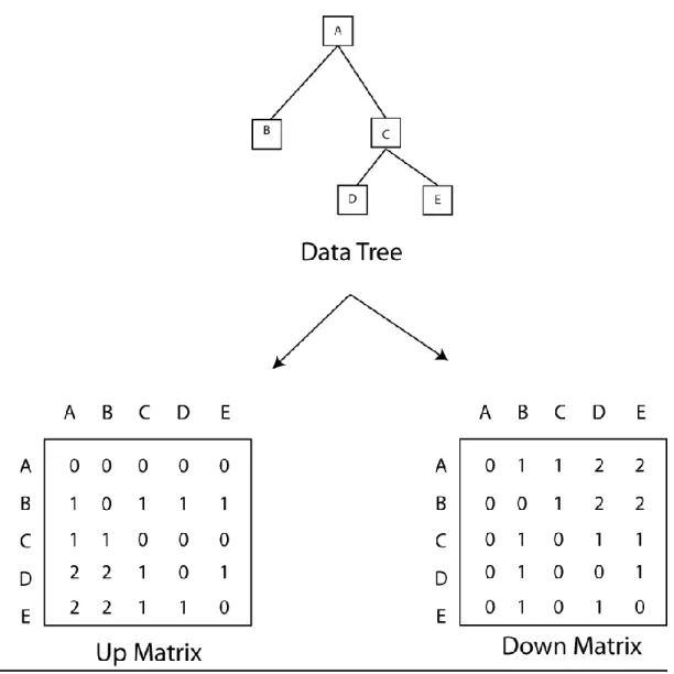
A potential improvement to these existing methods was proposed by Wang et al. (2005a). Their method is referred to as the Updown method (or USim) and is a topological approach based on the number of up and down operations between nodes in a tree. Up and down operations between two nodes refer to the direction that you move along a tree to get from one node to the other (a down operation refers to going from a parent node to its child (or descendant) node and an up operation refers to moving in the opposite direction). In this method, this convention is used to compute an Up matrix and Down matrix for each tree in a comparison. Figure 11 illustrates the process of generating both the Up and Down matrices from a given phylogenetic tree. Looking at the Up matrix first, we can see that since A is the root of the tree, it has no “up” operations to get to any of the other nodes. However, looking at node “C”, we can see that it takes one “up” operation for it to get to node A or node B (since when traversing the tree to get from C-B, we have to go to A and then to B). Conversely, there are no “up” operations required to go from C to D or E since those nodes are descendants of C. Looking at C again in

construction of its row in the “down” matrix, we see that there is one down operation to go from C to D and from C to E since those are child nodes of C and there is also 1 down operation required to go from C to B (since the path is from C->A->B and B is a child node of A). Since C is a descendant of A, there are no down operations required to go from C to A. It can be seen that the up matrix can be generated from the down matrix and vice-versa with the down matrix being equal to the transpose of the up matrix.

Provided these matrices for both trees in a comparison, the Updown distance between the two trees can be calculated. Since we have seen from above that the Up matrix and Down matrix are related to each other with one being the transpose of the other, only the up matrix (U) is used in the equations for computing the Updown distance. To compute this distance, for the

(29)

22

Figure 11 – Updown Diagram

Shows a phylogenetic tree and its corresponding Up and Down matrices. The updown distance(USIM value) between two trees is computed using these updown distance matrices from each tree in a comparison (Wang et al. 2005a).

set of labeled nodes in Q and Vd the set of labeled nodes in D. In calculating the Updown

(30)

23

Updown distance(Q,D) = ∑∑ [ ] [ ] ∑∑ [ ] (2)

Then, in order to compute the similarity score between Q and D, denoted USim (the metric actually used in this paper in future sections), the following equation is given:

USim(Q,D) = ( ( )_∑ _∑ _{[ ]}

) x 100% (3)

(31)

24

1.11 Possible Areas for Improvement on Existing Methods

While these methods have been extensively studied and are effective in certain cases, they can also be somewhat limited, especially in regard to the specific problem of searching large databases to find an effective ranking of phylogenies presented therein. PAR, while

computationally efficient with respect to tree size, does not offer a good distribution of similarity scores and is highly sensitive to the topology of the tree. Thus, while two trees might differ with only respect to a small number of nodes, the partitions created by these nodes can be very different and thus the two trees could be considered very distant (Bryant et al. 2000). MAST offers a simple means of visualizing the comparison of two trees, but it is not time efficient and does not offer the resolution necessary to implement as a search with a large database of trees. Quartet and NNI offer a relatively high resolution of similarity measures when comparing large trees, however both can be computationally intensive and in the case of NNI, it has proven to be an NP-hard problem (DasGupta 2000), and while studies have been done to try to improve and optimize an algorithm for accurately approximating this distance (Hon and Lam 2000), it is still computationally difficult and may not be effective for searching large databases for similar tree structures. The Updown distance metric is an improvement on these methods, but from the analysis that we will show, the implementation of the method does not scale well with regards to the size of the tree.

(32)

25

for the edge lengths (evolutionary distance) between nodes, omitting trees containing this key evolutionary information can limit the effective use of any comparison method.

(33)

Chapter 2 Methods and Results

2.1 Introduction to MDS-Procrustes

Our MDS-Procrustes approach begins by generating a distance matrix directly from a given phylogenetic tree’s alignment information. We then generate a high-dimensional Euclidean structure that represents the nodes as points in a high-dimensional space while still closely approximating their distance relationships via classical multi-dimensional scaling (MDS). For a comparison between two phylogenetic trees, this Euclidean structure will be generated for both trees and then we will superimpose one structure onto the other with a Procrustean approach. The degree of similarity between two trees is represented by a least-squares sum of deviations between corresponding point pairs. This distance approach should be an improvement to the topological approaches since it will not be as sensitive to the existence of particular branches in a tree when determining similarities.

(34)

27

2.2 Classical Multidimensional Scaling

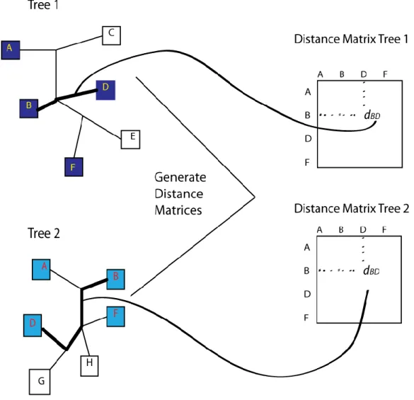
Consider two trees T1 and T2. T1 contains a set of nodes N = {n1,n2,…..,nn} and T2 contains a set of nodes M = {m1,m2,….,mm}. We generate distance matrices D1(nxn) and D2(mxm) such that dij for all i,j represents the patristic distance between node ni -> nj and mi -> mj respectively. This distance is computed following the paths of the branches connecting the nodes, and thus for weighted trees, this distance will include any weights assigned to an edge length. In order to be able to compare trees of different sizes and labels, at this point, we need to reduce and align the distance matrices D1 and D2 so that only the distances between nodes common to both trees are preserved. Figure 12 shows two trees and their corresponding distance matrices that result after removing nodes not common to both trees (These reduced matrices are referred to as R1 and R2).

After generating the distances between the nodes in each tree, we take these reduced distance matrices and represent them in a Euclidean space via classical MDS. To do this for each tree, we take the reduced distance matrix R and find the contrast matrix B such that B = where J is the centering matrix ( is the number of nodes and 1 is a row vector of ones) and is equal to the reduced distance matrix R. We then perform

eigendecomposition of B = to get the coordinate matrix (Borg and Groenen 2005). The solution is given by:

(35)

28

Figure 12 - Generating Distance Matrices

Generate distance values between each pair of nodes within a tree by following along the paths on tree. The matrices R1 and R2 are found by looking at only the nodes common to

both trees in a comparison.

(36)

29

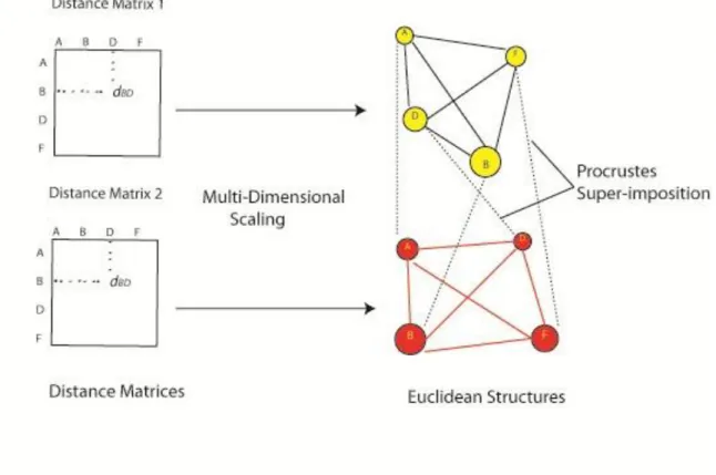
2.3 Procrustes Superimposition of Two Euclidean Structures

After obtaining the coordinate matrices X1 and X2 for each of the trees in a comparison, we perform a Procrustean superimposition on the matrices to determine their degree of similarity. This superimposition can be performed on two sets of points of the same size (prior to this, if X1 and X2 are not of the same dimensionality, we add columns of 0s to the appropriate matrix to align them) Y1 and Y2. Procrustes will compute the optimal linear transformation by minimizing

‖ ‖ where is the transformation matrix. Here, Y1 is superimposed onto Y2 by means of applying C (translation), R (rotation and reflection) and B (scaling) to Y2. This will be minimized when the following conditions are true:

, ( )

( ) ,

( )

(5)

Where and are orthogonal matrices derived from the singular value decomposition of

(37)

30

Figure 13 - Procrustes with Euclidean Structures

Take distance matrices from each tree and represent the nodes as points on a high-dimensional Euclidean structure which maintains the distance relationships provided in matrix. Then, use Procrustes super-imposition to align the two structures to one another to find a similarity score.

2.4 Implementation and Initial Testing

(38)

31

To accomplish this, we generated a set of 40 unweighted, unrooted data trees D = {d1,…..,d40} with Ndata = {n1,…..,n20} nodes. The trees were generated using the rtree function from the Ape package in R. We then selected a random Nquery={nm,…,nm+4} with m ≤ 16 for each d in D to comprise our set of query trees Q = {q1,…..,q40}. Thus, each query tree would always be a random 5 node subtree of a data tree. We then compared each qεQ to each dεD to test the ability of our method to correctly detect similarity between a tree and its subtree as a query structure.

In this scenario, MDS-Procrustes was able to correctly identify the most similar data tree as the structure from which the query tree was derived each time (with a distance equal to 0 on each instance). This is expected since we reduce the input distance matrices to include only distances between common nodes prior to MDS and Procrustes analysis, but it is important to show that the method will work for the trivial case and that the fitting will not yield any

(39)

32

Figure 14 - MDS-Procrustes distribution for validation dataset

Similarity score distribution for random data set of 40 weighted trees with 20 nodes. Query tree used was a random 5 node subtree of each given data tree in the comparison. The 40 100% similarity matches represent the situation when the query tree was compared to the data tree from which it originated.

(40)

33

query. Figures 18 and 19 show the second ranked full tree and its subtree used in the comparison with the query tree from figure 15. The similarity score for this comparison was 0.1796, a relatively high degree of similarity. As illustrated in the figures, while not identical in structure, these two trees are actually highly related in terms of the distances between their common nodes. This is an important distinction to make with regards to a fundamental difference between

topological searches and distance-based searches, as topological searches may not be able to resolve the fact that these two trees are similar since the nodes were in different positions in the two trees. However, here, we measure similarity as a function of the distance between the nodes, so the position of the node in the original tree is not of specific consequence, only its position relative to the other nodes is relevant. Being overly sensitive to the original location of particular taxa in a given phylogenetic tree can cause many trees of similarity to be considered dissimilar and is a somewhat limiting aspect to many topologically based tree comparison methods.

(41)

34

Figure 15 – Random Search Query

Query Tree used in random tree search and compared to 40 different randomly generated trees.

Figure 16 – Random Search Top Ranker

(42)

35

Figure 17 – Random Search Top Rank Subtree

Subtree used in MDS-Procrustes comparison between trees from Fig 15 and Fig 16. It can be easily seen that this subtree matches up exactly with Fig 15, thus the 100% similarity.

Figure 18 – Random Search Second Ranker

(43)

36

Figure 19 – Random Search Second Ranker Subtree

Subtree used in MDS-Procrustes between trees from Fig 1 and Fig 5. The MDS-Procrustes distance between these trees was found to be 0.176 and this similarity can be observed from the pictures by looking at the similarity in the distances between the sets of nodes.

2.5 Data Sets

In our analysis, we will take a similar approach to the work performed by Wang et al.(2005a) and show how MDS-Procrustes compares to the previously described methods. Initially, we will use synthetically created data to compare the distribution of similarity scores between the methods and then also look at the efficiency with respect to tree size for each method to compute the similarity scores for a given set of data trees. Here, we use the Component tool (Page 2001) to implement the NNI, PAR, MAST and Quartet metrics. The USim (UpDown) metric was implemented using a Java program from Wang et al. (2005b) and was slightly

(44)

37

of the different methods. As indicated in the previous section, we use Matlab code to perform all comparisons with MDS-Procrustes.

Our method-comparison experiment used two separate sets of data trees to comprise sample databases of trees. In the initial set, the database consists of 300 unrooted, labeled trees with 8 nodes. We compared the distances/similarities among all of the trees in the given set and output the results into histograms to view the similarity score distribution of each method. A wide distribution of scores is needed to be able to effectively rank trees, otherwise several tree comparisons can generate the same score(s) and a method will not be able to distinguish between them in terms of similarity. The second database of trees consisted of 300 unrooted, labeled trees with 20 nodes. As previously noted, several methods can offer good score distribution when comparing trees with a large number of nodes, and thus we compared the similarity score outputs on trees of differing sizes to analyze this further (as searching large databases of trees effectively would optimally require resolution for both large trees and small trees).

2.6 Method Metric Distributions for Initial Data Set

Figures 20-25 show the distribution of similarity scores (metrics) for each of the

described methods for the initial set of data. As theorized previously, PAR and MAST offer very low resolutions in this situation, each method only able to bin all of the comparisons into six separate bins. This would make it ineffective to use these metrics as a basis for ranking trees in terms of their similarity to a given query tree since a large number of trees would contain the same degree of similarity. NNI and Quartet offer a better distribution of scores in this case, but both distributions are not as good as those provided by the Updown and MDS-Procrustes

(45)

38

information is known), it shows that even with small trees, MDS-Procrustes is at least as effective as any of the tested metrics (and in many cases, it offers significantly improved score

distribution).

Figure 20 – PAR distribution for initial dataset

(46)

39

Figure 21 – MAST distribution for initial dataset

Distribution of MAST metric values for comparison of tree distances among 300 8 node trees.

Figure 22 – NNI Distribution for initial dataset

(47)

40

Figure 23 – Quartet distribution for initial dataset

Distribution of Quartet metric values for comparison of tree distances among 300 8 node trees.

Figure 24 – Usim distribution for initial dataset

(48)

41

Figure 25 – MDS-Procrustes distribution for initial dataset.

Distribution of MDS-Procrustes metric values for comparison of tree distances among 300 8 node trees.

Another aspect to consider in measuring the effectiveness of each method is how often the methods find an exact match in similarity to the data tree. Since our dataset had 300 different randomly generated trees, we would expect to see only 300 exact matches (only when the query tree was compared to itself out of the dataset). However, this was not the case in NNI, Quartet, or PAR. Each of those methods found 302 exact matches, indicating that there were two sets of trees that were found to be 100% similar even though they were not exactly the same tree.

(49)

42

relatively high degree of similarity between the trees (as would be expected), it does not detect them as 100% similar. Updown and MAST also detect the trees as different, with varying degrees of similarity.

In this particular example, the figures show that the trees actually have the same sets of nodes directly connected to one another, however the relation of these sets to one another is different and thus the trees are not the exact same. NNI, Quartet and PAR are unable to resolve these differences since each of those methods essentially look only at relationships at interior edges and do not look at the relation of each node individually to the entire tree. So, while the presence of this type of error decreases as the trees get larger, it is clear that there are some minor resolution issues with comparing trees of relatively small size with those methods. This also further demonstrates the effectiveness of MDS-Procrustes in terms of ranking trees according to similarity as it is able to resolve minor differences between trees as good or better than any of the existing topological methods.

Figure 26 – Exact Match Tree 1.

(50)

43

Figure 27 – Exact Match Tree 2.

Tree diagram for Tree that is exact match to Figure 20 according to NNI, Quartet, and PAR metrics but not according to MDS-Procrustes.

2.7 Method Metric Distributions for Second Data Set

(51)

44

Figure 28 – Par Distribution for second dataset

Distribution of Partition metric values for comparison of tree distances among 300 20 node trees.

Figure 29 – MAST distribution for second dataset

(52)

45

Figure 30 – NNI distribution for second dataset

Distribution of NNI metric values for comparison of tree distances among 300 20 node trees.

Figure 31 – Quartet distribution for second dataset

(53)

46

Figure 32 – Updown Distribution for second dataset

Distribution of Updown method metric (USim) scores for comparison of tree distances among 300 20 node trees.

Figure 33 – MDS-Procrustes distribution for second dataset

(54)

47

Furthermore, it can be seen that with a greater number of nodes in the trees, the occurrence of a tree finding another tree with 100% similarity to itself is eliminated in all methods, as the only comparisons resulting in trees being 100% similar occur when the tree is compared to itself . In combining the results here with the results from the initial data set, it is clear that only MDS-Procrustes, USim, and Quartet offer good enough resolution to effectively rank similar trees in both the small and larger tree scenarios.

2.8 Method Computation Performance with Varying Tree Size

Since tree databases can often contain trees very large in size, time scaling with respect to the size of the tree is an important aspect of any comparison method. With many topological searches, the increase in time with respect to the size of the tree is large, as the presence of additional nodes/branches presents many more possible solutions and thus requires a great deal of computational time to process (which can offset the resolution improvement provided by the inclusion of more nodes). We will initially provide the reported time complexity for each of the methods used and then perform runtime tests with trees of varying sizes to see which method(s) perform best with regards to time when varying the tree size.

The partition metric is computationally fast and as implemented here, the time complexity is O(n) (Critchlow 1996). This is to be expected since the method simply lists all partitions found in both trees and then compares them together to determine the degree of

(55)

48

The Quartet method used here can compute the quartet distance in O(n3) time, which is the same computational complexity of the proposed MDS-Procrustes algorithm. Also, as previously stated, the NNI distance between two trees cannot be computed in polynomial time, however the approximation used here computes this distance by rooting each tree at each node and transforming one tree into the other beginning at each of these points and then determining the minimum nni distance by taking the minimum of these values. This approximation requires O(n log10 n) time to compute for rooted trees and O(n2 log10 n) for unrooted trees (Brown and Day 1984). The computational complexity for the Updown distance metric is O(n2+ m) where n is the number of nodes in the query tree and m is the number of nodes in the data tree (thus, in all comparisons in this paper since we used trees with the same nodes, the complexity would be n2 +

n).

Beyond looking at the computational complexity of each algorithm, we now want further analyze each method’s runtime as a function of tree size here. In this test, we looked at 100 unrooted and unweighted trees, ranging in size from five nodes to fifty nodes. For each run, we compared each tree to every other tree in the set and calculated the run-time in seconds of the total search of 4950 comparisons. All programs were run on a Windows Lenovo ThinkCentre workstation with an Intel Core 2 2.13 GHz CPU.

(56)

49

comparing varying sizes of trees, but its limitations with respect to distribution scores make it highly limited in its effectiveness in a comparison among large sets of trees. MDS-Procrustes performed well in both providing a highly-resolved distribution of similarity scores while also maintaining a relatively fast runtime with respect to the tree size, a highly desirable quality when searching through tree databases with large number of trees of varying nodes/sizes. It should be noted, that we would expect the MDS-Procrustes method time complexity to grow similar to the other topological methods at some point in time (when the size reaches a certain point), since their computational complexities are of the same or similar order. However, due to initial bias in the implementations of the methods, MDS-Procrustes did not begin displaying that time increase at the size that we reached here and while tests can be run on trees of greater size it is important to see how this method performed on moderately sized trees relative to the other methods.

(57)

50

Figure 34 – Runtime Comparison

Run times for each described method in comparison of similarity among 100 unweighted and unrooted trees. The tree size varied from 5-50 nodes.

(58)

Chapter 3 Conclusion and Future Work

3.1 Comparison Method Conclusion

In this work, we have introduced a novel method for comparing phylogenetic trees by viewing them as Euclidean structures in a high dimensional space and fitting them with a Procrustean approach. We have shown through the use of several sets of synthetic data that the application of this method produces a wide similarity score distribution making it effective in resolving tree similarities among different trees in a database. While other methods exist to achieve this same goal, we have seen that MDS-Procrustes offers a good distribution of similarity scores and time performance that is unmatched by several existing methods found in the

literature.

(59)

52

nodes. This is a desirable feature to have in a phylogenetic tree comparison algorithm as tree databases will have thousands of trees with different species/nodes and being limited to searching only those that contain the same sets of leaves would result in a limited application of any

proposed method.

Also, here we offer a method that contains an inherent extension for the comparison of weighted trees, an area in which many existing methods fail to address. Two of the methods discussed, NNI and Updown, contain extensions for including weighted trees. For NNI, an operation is charged a cost equal to the weight of the branch associated with it and while this has been proven effective, it adds to the computational time of a particular comparison (Hon and Lam 1999). Wang et al. presented an extension for supporting weighted trees in their Updown

approach; however this was not made available in their Java implementation for further study and evaluation here. PAR, MAST, and Quartet do not have natural extensions towards the support of weighted trees and thus cannot utilize any evolutionary distance information to refine their comparisons. Since we provide a method that generates a distance matrix directly from the node information provided, MDS-Procrustes inherently computes weights with no added

computational time to process the comparison (and we’ve already shown that our implementation is time efficient to other methods even in the unweighted case). Given the number of different algorithms available to generate these types of phylogenetic trees, this added functionality is another feature that allows for the proposed method to be useful in the comparison of many varied trees.

(60)

53

common subtree can have biological significance). MDS-Procrustes generates a similarity score based on the distances between nodes and how similarly those distances are resolved in both trees, but that distance does not contain a specific meaning, so in a one-to-one comparison, the MDS-Procrustes distance is not particularly useful other than to give a general indication of similarity. So, while MDS-Procrustes has been shown here to be effective in determining similarity when comparing a tree to a large set of trees and ranking the trees from that set by degree of similarity, some of the other topological methods (specifically MAST, Quartet and Partition) might be more useful when comparing one tree to another to determine exactly how the trees are similar and derive meaning from that similarity.

3.2 Future Work

The work here has shown MDS-Procrustes to potentially be very useful for the purposes of comparing a phylogenetic tree to a database of phylogenetic trees and being able to rank the results by degree of similarity. Here we used various forms of synthetically created data to create artificial databases and determine the effectiveness of the method(s), and since MDS-Procrustes performed well in comparison to other methods in this case, the next step would be to actually implement the method on one of the many phylogenetic tree databases in existence today (such as TreeBase).

(61)

54

(62)

55

References

[1] Borg I and Groenen P. 2005. Modern Multidimensional Scaling Theory and Applications, 2nd edition. Springer Science+Business Media, Inc. New York, NY.

[2] Brown E and Day W. 1984. A computationally efficient approximation to the nearest neighbor interchange metric. Journal of Classification, 1(1), 93-124.

[3] Bryant D, Tsang J, Kearney P and Li M. 2000. Computing the quartet distance between evolutionary trees. In Proceedings of the 11th Annual ACM-SIAM Symposium on Discrete Algorithms.

[4] Choi K. and Gomez S. 2009. Comparison of phylogenetic trees through alignment of embedded evolutionary distance. BMC Bioinformatics 2009, 10:423.

[5] Crichlow D, Pearl D, Qian C 1996. The triples distance for rooted bifurcating phylogenetic trees. Syst. Biol., 45(3), 323-334.

[6] Currie C, Wong B, Stuart A, Schultz T, Rehner S, Mueller U, Sung G, Spatafora J, Straus N 2003. Ancient tripartite coevolution in the attine ant-microbe symbiosis. Science 2003, 299,386-388.

[7] DasGupta B, He X, Jiang T, Li M, Tromp J. 2000. On computing the nearest neighbor interchange distance. In Proc. DIMACS Workshop on Discrete Problems with Medical

Applications, DIMACS Series in Discrete Mathematics and Theoretical Computer Science, Am. Math. Soc., 55, 125-143.

[8] Day W. 1983. Properties of the Nearest Neighbor Interchange Metric for Trees of Small Size. J. Theor Biol., 101, 275-288.

(63)

56

[10] Felsenstein J. 2003. Inferring Phylogenies. Sinauer Associates, Inc., Publishers, Sunderland, MA.

[11] Gordon A. 1979. A measure of the agreement between rankings. Biometrika(66), 7-15.

[12] Gower J and Dijksterhuis G. 2004. Procrustes Problems. Oxford University Press Inc.,Oxford, NY

[13] Hon W and Lam T. 1999. Approximating the Nearest Neighbor Interchange Distance for Evolutionary Trees with Non-Uniform Degrees. COCOON ’99, 1627, 61-70.

[14] Keselman D and Amir A. 1994. Maximum agreement subtree in a set of evolutionary trees: Metrics and efficient algorithms. In Proceedings of the 35th Annual Symposium on Foundations of Computer Science, 758-769.

[15] Kubicka E, Kubicki G, McMorris F.R. 1995. An algorithm to find agreement subtrees.

Journal of Classification, 12, 91-99.

[16] Lee C, Hung L, Chang M, Shen, C, Tang C. 2005. An improved algorithm for the maximum agreement subtree problem. Information Processing Letters, 94(5), 211-216.

[17] MacLeod D, Charlebois R, Doolittle F, Bapteste E 2005. Deduction of probable events of lateral gene transfer through comparison of phylogenetic trees by recursive consolidation and rearrangement. BMC Evolutionary Biology 2005, 5:27.

[18] Page, R. 2001. http://taxonomy.zoology.gla.ac.uk/rod/cpw.html.

[19] Pazos F. and Valencia A. 2001. Similarity of phylogenetic trees as indicator of protein-protein interaction. Protein Engineering, 14(9), 609-614.

(64)

57

[21] Saitou N and Nei M. 1987. The neighbor-joining method: A new method for reconstructing phylogenetic trees. Molecular Biology Evol, 4(4), 406-425.

[22] Sanderson M, Donoghue M, Piel W and Eriksson T. 1994. TreeBASE: A prototype database of phylogenetic analyses and an interactive tool for browsing the phylogeny of life. American Journal of Botany, 81(6), 183.

[23] Steel M and Penny D. 1993. Distributions of tree comparison metrics – some new results.

Systemic Biology, 42(2), 126-141.

[24] Stissing M, Pedersen C, Mailund T, Brodal G and Fagerberg R. 2006. Computing the quartet distance between evolutionary trees of bounded degree. In Proceedings of the 5th Asia-Pacific Bioinformatics Conference, 101-110.

[25] St John K, Warnow T, Moret B and Vawter L. 2003. Performance Study of Phylogenetic Methods: (Unweighted) Quartet Methods and Neighbor-Joining. Journal of Algorithms, 48(1), 173-193.

[26] Wang J, Shan H., Shasha D., Piel W. 2005a. Fast Structural Search in Phylogenetic Databases. Evolutionary Bioinformatics Online 2005,1, 37-46.

[27] Wang J, Regula S, Shasha D, Hua L and Patel R. 2005b.

http://web.njit.edu/~wangj/updown.htm.