The handle
http://hdl.handle.net/1887/85675
ho
lds various files of this Leiden University
dissertation.
Author
:
Shan, H.
Title
:
Towards high performance and efficient brain computer interface character speller :
convolutional neural network based methods
Brain Computer Interface Character Speller:
Convolutional Neural Network based Methods
Convolutional Neural Network based Methods
PROEFSCHRIFT
ter verkrijging van
de graad van Doctor aan de Universiteit Leiden, op gezag van Rector Magnificus Prof.mr. C.J.J.M. Stolker,
volgens besluit van het College voor Promoties te verdedigen op woensdag 25 februari 2020
klokke 16:15 uur
door
Hongchang Shan geboren te Heilongjiang, China
Promotion Committee: Prof. Dr. Tom Heskes Radboud Universitiet
Prof. Dr. Shaowei Cai Chinese Academy of Sciences Prof. Dr. Holger Hoos Universiteit Leiden
Prof. Dr. Fons Verbeek Universiteit Leiden Dr. Wojtek Kowalczyk Universiteit Leiden
Towards High Performance and Efficient Brain Computer Interface Character Speller: Convolutional Neural Network based Methods Hongchang Shan.
-Dissertation Universiteit Leiden. - With ref. - With summary in Dutch.
Copyright c2020 by Hongchang Shan. All rights reserved. No part of this thesis may be reproduced, stored in a retrieval system, or transmitted in any form or by any means, electronic, mechanical, photocopying, recording or otherwise without prior permission from the author.
Contents v
List of Tables ix
List of Figures xiii
List of Abbreviations xv
1 Introduction 1
1.1 Development Trends in P300-based Brain Computer Interface Systems 2 1.1.1 High Performance P300-based Brain Computer Interface
Sys-tems . . . 2
1.1.2 Efficient P300-based Brain Computer Interface Systems . . 4
1.2 Problem Statement . . . 6
1.2.1 Problem 1 . . . 7
1.2.2 Problem 2 . . . 8
1.3 Research Contributions . . . 9
1.4 Dissertation Outline . . . 13
2 Background 15 2.1 Machine Learning . . . 15
2.2 Neural Network . . . 17
2.2.1 Neurons . . . 17
2.2.2 The Architecture of a Neural Network . . . 19
2.2.3 Learning Process of a Neural Network . . . 22
2.3 Convolutional Neural Network . . . 27
2.3.1 The Convolution Operation . . . 29
2.3.2 The Characteristics of Convolutional Neural Network . . . . 29
2.3.3 The Architecture of Convolutional Neural Network . . . 30
2.4.1 P300 Signal . . . 31
2.4.2 P300 Speller . . . 33
2.4.3 Performance Assessment of P300 Speller . . . 34
2.5 Datasets . . . 35
3 A Simple Convolutional Neural Network for P300 Signal Detection and Character Spelling 39 3.1 Related Work . . . 41
3.2 Proposed Convolutional Neural Network . . . 44
3.2.1 Input to the Network . . . 44
3.2.2 Network Architecture . . . 45
3.2.3 Training . . . 47
3.3 Experimental Evaluation . . . 48
3.3.1 Experimental Setup . . . 48
3.3.2 Complexity . . . 48
3.3.3 P300 Signal Detection Accuracy . . . 49
3.3.4 Character Spelling Accuracy . . . 50
3.3.5 Information Transfer Rate . . . 52
3.4 Conclusions . . . 55
4 Ensemble of Convolutional Neural Networks for P300 Signal Detection and Character Spelling 57 4.1 Proposed Network . . . 59
4.1.1 Ensemble of Convolutional Neural Networks . . . 59
4.1.2 Proposed OSLN and OTLN . . . 59
4.1.3 Training . . . 61
4.1.4 P300 Signal Detection and Character Spelling using EoCNN 61 4.2 Experimental Evaluation . . . 62
4.2.1 Complexity . . . 63
4.2.2 P300 Signal Detection Accuracy . . . 63
4.2.3 Character Spelling Accuracy . . . 64
4.2.4 Information Transfer Rate . . . 67
4.3 Discussions . . . 69
4.3.1 Analysis of Our Proposed OTLN and OSLN . . . 69
4.3.2 Ablation Study on EoCNN . . . 71
4.3.3 Exploration on the Importance of Extracting P300-related Fea-tures from Raw Signals . . . 72
5 A Novel Sensor Selection Method based on Convolutional Neural Network
for P300 Speller 75
5.1 Related Work . . . 77
5.2 Our Sensor Selection Method . . . 78
5.2.1 Spatial Learning based Elimination Selection . . . 78
5.2.2 Parameterized OSLN . . . 79
5.2.3 Ranking Function . . . 81
5.3 Experimental Evaluation . . . 82
5.3.1 Experimental Setup . . . 82
5.3.2 Experimental Results . . . 84
5.4 Discussions . . . 85
5.4.1 Configuration ofEsin SLES . . . 86
5.4.2 Exploring the Impact of the CNN Architecture on Sensor Se-lection . . . 88
5.5 Conclusions . . . 92
6 An Improved Ensemble of Convolutional Neural Networks for P300 Speller with a Small Number of Sensors 95 6.1 Study on EoCNN-based P300 Speller with Different Number of Sensors 97 6.1.1 Experimental Setup . . . 97
6.1.2 Experimental Results . . . 98
6.2 Our Solution Approach . . . 100
6.2.1 Parameterized Ensemble Processing . . . 100
6.2.2 Parameter Configuration for Parameterized Ensemble Process-ing . . . 101
6.3 Experimental Evaluation . . . 103
6.3.1 Experimental Setup . . . 103
6.3.2 Experimental Results . . . 105
6.4 Conclusions . . . 108
7 Summary and Conclusions 109
Bibliography 113
List of Publications 121
Samenvatting 123
Acknowledgments 127
2.1 Number of P300s/non-P300s for each dataset. . . 37
3.1 CCNN architecture. . . 43
3.2 BN3 architecture. . . 43
3.3 CNN-R architecture. . . 44
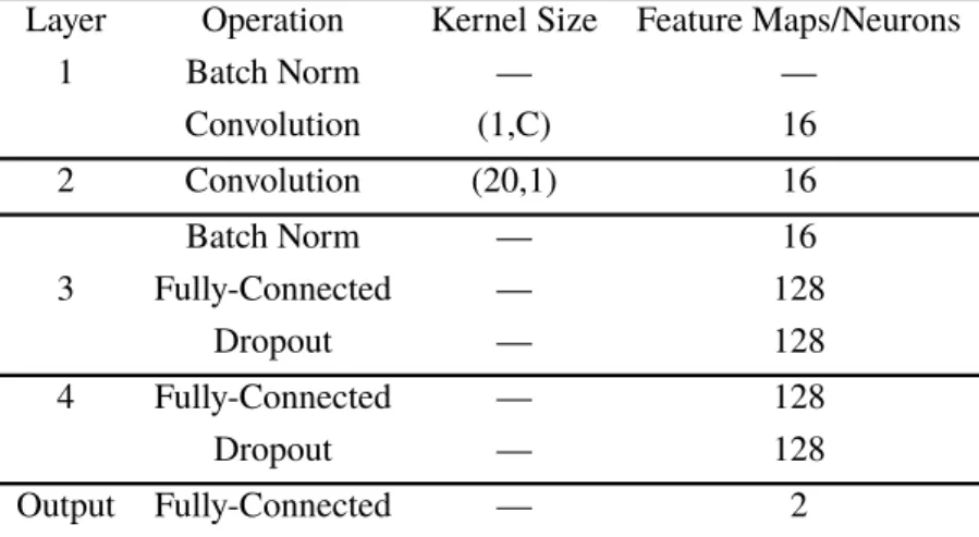
3.4 OCLNN architecture. . . 46
3.5 Complexity comparison of different CNNs. . . 49
3.6 P300 signal detection accuracy of different CNNs on Dataset II, III-A and III-B. . . 50
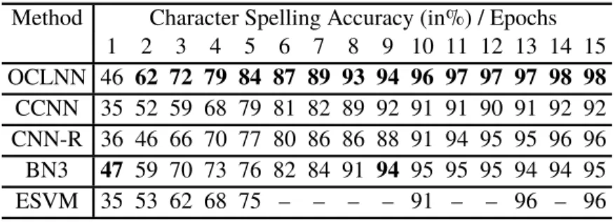
3.7 Spelling accuracy achieved by different methods on Dataset II. . . . 51
3.8 Spelling accuracy achieved by different methods on Dataset III-A. . 51
3.9 Spelling accuracy achieved by different methods on Dataset III-B. . 51
3.10 Spelling accuracy achieved by OCLNN when using and not using the Batch Normalization operation on Dataset II. . . 53
3.11 Spelling accuracy achieved by OCLNN when using and not using the Batch Normalization operation on Dataset III-A. . . 53
3.12 Spelling accuracy achieved by OCLNN when using and not using the Batch Normalization operation on Dataset III-B. . . 53
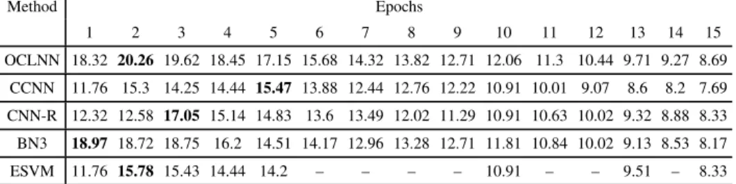
3.13 The ITR of the P300 speller based on different methods on Dataset II. 54 3.14 The ITR of the P300 speller based on different methods on Dataset III-A. . . 54
3.15 The ITR of the P300 speller based on different methods on Dataset III-B. . . 54
4.1 OSLN architecture. . . 60
4.2 OTLN architecture. . . 60
4.3 Complexity of different CNNs. . . 63
4.5 Spelling accuracy achieved by different methods on Dataset II. . . . 65
4.6 Spelling accuracy achieved by different methods on Dataset III-A. . 65 4.7 Spelling accuracy achieved by different methods on Dataset III-B. . 66
4.8 The ITR of the P300 speller based on different methods on Dataset II. 67
4.9 The ITR of the P300 speller based on different methods on Dataset III-A. . . 67
4.10 The ITR of the P300 speller based on different methods on Dataset III-B. . . 68
4.11 Spelling accuracy achieved by OTLN, OSLN and EoCNN on Dataset III-A. . . 70
4.12 Spelling accuracy achieved by EoCNN after removing a separate CNN. 71
5.1 The symbols used in Algorithm 1. . . 79
5.2 OSLN(S)architecture. . . 81
5.3 Methods compared with SLES. . . 83 5.4 Minimal number of sensors selected by different methods for Dataset
II. The P300 speller is implemented using the CNN-based classifier OCLNN. . . 85
5.5 Minimal number of sensors selected by different methods for Dataset III-A. The P300 speller is implemented using the CNN-based classi-fier OCLNN. . . 86
5.6 Minimal number of sensors selected by different methods for Dataset III-B. The P300 speller is implemented using the CNN-based classi-fier OCLNN. . . 87 5.7 Minimal number of sensors selected by different methods for Dataset
II. The P300 speller is implemented using the CNN-based classifier EoCNN. . . 88
5.8 Minimal number of sensors selected by different methods for Dataset III-A. The P300 speller is implemented using the CNN-based classi-fier EoCNN. . . 89
5.9 Minimal number of sensors selected by different methods for Dataset III-B. The P300 speller is implemented using the CNN-based classi-fier EoCNN. . . 90 5.10 Minimal number of sensors selected by different methods for Dataset
II, The P300 speller is implemented using the SVM-based classifier ESVM [RG08]. . . 91
5.12 Minimal number of sensors selected by different methods for Dataset III-B, The P300 speller is implemented using the SVM-based classi-fier ESVM [RG08]. . . 93 5.13 Minimal number of sensors selected by SLES with differentEs
con-figurations. . . 94 5.14 Minimal number of sensors selected by analysing different CNNs. . 94
6.1 Minimal number of sensors needed to acquire EEG signals in the P300 speller based on different CNNs without losing the state-of-the-art spelling accuracy of the P300 speller on Dataset II. . . 105 6.2 Minimal number of sensors needed to acquire EEG signals in the
P300 speller based on different CNNs without losing the state-of-the-art spelling accuracy of the P300 speller on Dataset III-A. . . 106 6.3 Minimal number of sensors needed to acquire EEG signals in the
P300 speller based on different CNNs without losing the state-of-the-art spelling accuracy of the P300 speller on Dataset III-B. . . 106 6.4 Minimal number of sensors needed to acquire EEG signals in the
1.1 Workflow of a typical BCI. . . 1
1.2 An example of a traditional P300-based BCI system. . . 5
1.3 An example of an efficient P300-based BCI system. . . 5
2.1 The workflow of machine learning. . . 17
2.2 The model of a neuron. . . 18
2.3 Architectural graph to model a neuron. . . 20
2.4 An example of a single-layer neural network. . . 21
2.5 An example of a multi-layer neural network with one hidden layer and one output layer. . . 21
2.6 An example of a cost functionCwith two parametersv1andv2. . . 23
2.7 The analogy of using gradient descent to minimize a cost function. . 24
2.8 An example of the architecture of a CNN used for the handwritten digit recognition. . . 31
2.9 P300 signal. . . 32
2.10 P300 speller character matrix. . . 33
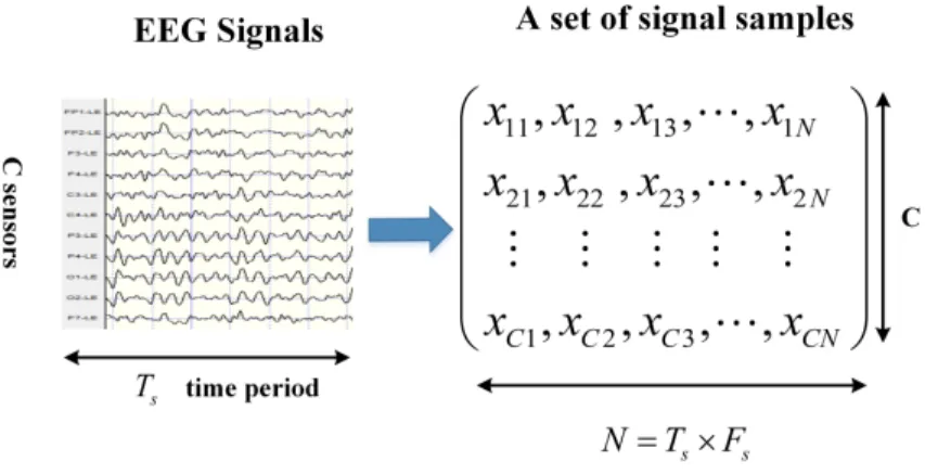
2.11 An example of a set of signal samples, whereFsis the signal sampling frequency . . . 36
3.1 Abstraction of the raw signals in the spatial convolution layer in cur-rent CNNs. xdenotes a signal sample in the input tensor. fdenotes a datum in a feature map. Every column in the input tensor contains a set ofCsignal samples. These samples come fromCsensor at a cer-tain sampling time point. The spatial convolution operation converts each column of spatial data (receptive field) from the input tensor into an abstract datum in a feature map. . . 42
3.2 Input tensor for our proposed OCLNN. . . 45
3.3 Illustration of OCLNN for P300 signal detection. . . 46
4.2 Spelling accuracy achieved by OTLN, OTLN-3l and OTLN-6l on Dataset III-A. . . 70 4.3 Spelling accuracy achieved by networks in set RAW_networks and
networks in set unRAW_networks on Dataset III-A. . . 72
5.1 Input tensor toOSLN(S), wheresj ∈S. . . 80 6.1 Spelling accuracy of different P300 speller implementations when
different number of sensorsmis used to acquire EEG signals. . . . 99 6.2 max-ITR of different P300 speller implementations when different
number of sensorsmis used to acquire EEG signals. . . 99 7.1 Overview of how each chapter’s contributions improve the
ALS Amyotrophic Lateral Sclerosis AP Action Potential
AUC Area Under the Receiver Operating Characteristic BCI Brain Computer Interface
CNN Convolutional Neural Network CWT Continuous Wavelet Transform DWT Discrete Wavelet Transform ECoG Electrocorticography EEG Electroencephalography
EoCNN Ensemble of Convolutional Neural Networks ERD Event Related Desynchronization
ERP Event-Related Potential FLD Fisher’s Linear Discriminants ITR Information Transfer Rate LDA Linear Discriminant Analysis LFP Local Field Potential
max-ITR maximum ITR MSE Mean Squared Error NN Neural Network
OCLNN One Convolution Layer Neural Network OSLN One Spatial Layer Network
OTLN One Temporal Layer Network
SAE Stacked Autoencoder SGD Stochastic Gradient Descent
SLES Spatial Learning based Elimination Selection SMAC Sequential Model-based Algorithm Configuration SNR Signal to Noise Ratio
SSNR Signal to Signal and Noise Ratio SSVEP Steady State Visual Evoked Potential SVM Support Vector Machine
SWLDA Stepwise Linear Discriminant Analysis II BCI Competition II - Data set IIb
Introduction
A
Brain Computer Interface (BCI), also known as mind-machine interface, trans-lates brain signals into computer commands, thereby building communication between the human brain and outside devices. In this way, human-beings can use only the brain to express their thoughts without any real movement. As a result, BCIs become an important communication pathway for the people who lose motor ability, such as patients with Amyotrophic Lateral Sclerosis (ALS) [SD06] or spinal-cord in-jury. In recent years, BCIs have also been popularly developed for healthy people, in application domains such as entertainments [GP+13], mental state monitoring [LTK13], virtual reality [CBJ16] as well as in IoT services [LL+14].A BCI system consists of three components, as shown in Figure 1.1. The first component is the brain signal acquisition. In this component, the brain signals of a subject (person) are recorded by using a brain headset equipped with a number of sensors. The acquired brain signals are sent to the second component for brain signal processing and translation. In this component, a hardware/software platform is used to process and translate brain signals into computer commands. Then, in the last component, the translated commands, i.e., the control signals, are used to control the outside devices, e.g., a prosthesis [MPP08], a computer mouse [Spü15], a mobile phone [CCH+10], or a robot [BFL13].
Figure 1.1: Workflow of a typical BCI.
sig-nals in the brain headset, BCI systems can be categorized as invasive BCIs, semi-invasive BCIs, and non-semi-invasive BCIs [Wal16]. In semi-invasive BCIs, micro-sensor arrays are placed directly into the cortex [PHP10] to measure action potentials (APs) and lo-cal field potentials (LFPs). In semi-invasive BCIs, sensors are placed on the exposed surface of the brain in order to measure electrocorticography (ECoG) signals [SL11]. In non-invasive BCIs, sensors are placed on the scalp in order to acquire electroen-cephalography (EEG) signals [GS06]. In recent decades, EEG-based BCIs attract most of the BCI research due to their non-invasive, easy, and safe way of acquiring brain signals. EEG-based BCIs can be divided in four main categories [FRAG+12], namely P300-based BCIs [FD88], steady state visual evoked potential (SSVEP)-based BCIs [Her01], event related desynchronization (ERD)-based BCIs [PN01], and slow cortical potential-based BCIs [BKG+00]. Compared with the other categories of EEG-based BCIs, the based BCIs have the following advantages. The P300-based BCIs are effective for almost every BCI user because the P300 signal, which is the target signal used in the P300-based BCIs, can be evoked in the brain of almost every human being [Els09]. In addition, the P300-based BCIs are relatively fast and straightforward to use. Moreover, the P300 signals work outstandingly well for BCI character spelling applications [GDS+09]. Therefore, the P300-based BCIs have at-tracted a lot of BCI researchers. As the benchmark for a P300-based BCI [FRAG+12], the P300 speller [FD88] has been the most-commonly investigated application of the P300-based BCI [FRAG+12]. Thus, this dissertation takes the P300 speller as the target BCI application.
1.1
Development Trends in P300-based Brain Computer
In-terface Systems
P300-based BCIs are still not used in human’s daily life and remain in an experimental stage at research labs. In order to bring P300-based BCIs into practical use, currently, there are two development trends for P300-based BCI systems, i.e., to design high per-formance P300-based BCI systems and to design efficient P300-based BCI systems.
1.1.1 High Performance P300-based Brain Computer Interface Systems
the P300 signals have a very low Signal to Noise Ratio (SNR). This makes it difficult to detect P300 signals evoked in the human’s brain, resulting in a low communication accuracy and speed of the P300-based BCI systems. P300-based BCI systems with such low performance are not acceptable for BCI users in their daily life. We take the P300 speller, the most-widely used application of the P300-based BCIs, as an exam-ple. Guy [GSB+18] explored the usability of the current P300 spellers for disabled people with amyotrophic lateral sclerosis. This report shows that when using a cur-rent P300 speller, half of the subjects (persons) cannot spell characters with accuracy that is higher than 90%. To promote P300 spellers to be used in people’s daily life, we should try our best to make the subjects spell characters with a P300 speller like the healthy people spell characters with their mouth. This means that we should try to make the subjects who use a P300 speller to achieve the character spelling accuracy that is (or close to) 100%. A P300 speller with accuracy that is much lower than 100% cannot be used in people’s daily life. In addition, Guy’s report [GSB+18] also shows that when using the current P300 spellers, the mean number of characters correctly spelled by the subjects is 3.6 characters per minute. However, a healthy person is able to speak with around 120 characters per minute. Compared with 120 characters per minute, the communication speed of the current P300 spellers, i.e., 3.6 characters per minute, is far from what is needed to be used in people’s daily life. Therefore, in-creasing the performance of the P300-based BCIs is a must in order to promote the P300-based BCIs into people’s daily life.
To increase the performance of a P300-based BCI system, efforts are focused on the signal acquisition part and on the signal processing and translation part of a BCI system. In the signal acquisition part, researchers try to improve the recording quality of the EEG signals such that the signals, that contain P300 evoked potentials, have less noise. For example, Koka [KB07] has developed tripolar concentric sensors. These sensors use advanced engineering techniques to enhance the recording capability for brain signals. Unfortunately, the current signal recording techniques cannot provide high enough SNR for P300 signals, thereby not guaranteeing alone very good perfor-mance of a P300-based BCI system.
ex-tract P300-related features. Researchers also try to remove artifacts in order to reduce the noise. For example, Gao [GZW10], Mennes [MWV+10], and Gwin [GG+10] propose signal processing methods to remove the artifacts caused by the muscle con-traction, the eye movement, and the body movement, respectively. In terms of classifi-cation methods for P300-based BCIs, researchers have tried different classifiers, such as Support Vector Machine (SVM) [KMG+04, RG08], Linear Discriminant Analy-sis (LDA) [JAB+10], Fisher’s Linear Discriminants (FLD) [SS09], Stepwise Linear Discriminant Analysis (SWLDA) [JK09], and neural networks (NN) [CG11, MG15, LWG+18, SLS18], in order to improve the accuracy of detecting P300 signals. The rapid development of machine learning algorithms for P300-based BCIs boosts the performance improvement for P300-based BCI systems.
1.1.2 Efficient P300-based Brain Computer Interface Systems
P300-based BCI systems have been in an experimental stage at research labs for a long time. Traditional P300-based BCI systems, as shown in Figure 1.2, use a complex EEG headset which utilizes a large number of sensors for brain signal acquisition as well as they use a cumbersome computer for signal processing and translation. Even though such BCI systems may achieve high enough performance in some cases, such complex systems for P300-based BCIs cannot be used in people’s daily life. This is because it is impossible for people who wear such complex headset and need such cumbersome computer to move freely everywhere they want. In order to bring P300-based BCIs into practical use, in recent years, researchers have been trying to develop efficient P300-based BCI systems. As shown in Figure 1.31, an efficient P300-based BCI uses a wireless EEG headset for signal acquisition. This headset utilizes a small number of sensors. In addition, such efficient BCI system uses a small mobile platform (e.g., mobile phone) for signal processing and translation. Since nowadays people use mobile phones almost every day and everywhere, it brings BCI users much conve-nience to use a mobile phone to process brain signals. Therefore, in recent years, a lot of research has been done for efficient P300-based BCI systems that use a wireless EEG headset for signal acquisition and a mobile phone for signal processing.
Concerning the wireless EEG headset, researchers have performed investigations to figure out the type of sensors as well as the number and the position of the sensors placed in the headset in order to build efficient P300-based BCI systems. Regarding the type of the sensors, traditional headsets, used in P300-based BCI systems, utilize wet sensors that operate with specially made conductive gels. The use of gels provides stable and high quality signal recording during a long-term use of a P300-based BCI system. However, the gels are sticky, which makes the BCI users’ hair dirty and also
1
Figure 1.2: An example of a traditional P300-based BCI system.
Figure 1.3: An example of an efficient P300-based BCI system.
sensors may impair the performance of the P300-based BCI systems because com-pared with wet sensors, dry sensors cannot provide the same high quality of recorded EEG signals, and non-contact sensors provide even lower quality of recorded EEG signals because non-contact sensors output a very small signal amplitude and they are very sensitive to artifacts [IS16].
In addition to the development of the aforementioned types of sensors, researchers also focus on reducing the number of sensors used in a P300-based BCI system while keeping the performance of this system acceptable [RG08, RS+09, RCP+10, CRC+10, CR+11, RCS+11, RCMM12, CRT+14]. These studies propose sensor selection meth-ods which select an appropriate sensor subset from an initial large set of sensors while keeping an acceptable BCI system performance. Such methods enable substantial re-duction of the sensors needed to acquire EEG signals. The rere-duction of the number of sensors in a P300-based BCI system decreases the price of the EEG headset signif-icantly, reduces the installation time of the P300-based BCI system, and also makes the users feel more comfortable. These advantages of the reduction of the sensors help promoting P300-based BCIs to be used in people’s daily life.
After acquiring EEG signals from a wireless EEG headset, an efficient P300-based system uses a small mobile platform, such as a mobile phone, to process these sig-nals. The mobile phone is an example of an embedded resource-constrained com-puting platform. Thus, the battery and memory of such platform are limited. As a result, the mobile phone cannot support the execution of signal processing algo-rithms with high complexity because such complex algoalgo-rithms consume too much energy and memory where the amount of this consumption exceeds the limits of a mobile phone. Therefore, in order to build efficient P300-based BCI systems, sig-nal processing algorithms with low complexity and acceptable performance are in urgent need. Such algorithms should be able to run on a mobile phone and con-sume a small amount of energy while keeping the system performance acceptable. In addition, in order to build energy-efficient P300-based BCI systems, techniques developed in the embedded system field can be used. Such techniques for energy-efficient task scheduling [LSWS16, CS16, NS17] and energy-energy-efficient application mapping [LSCS15, SLS16] help the mobile phone to work energy-efficiently when used in a P300-based BCI system.
1.2
Problem Statement
efficiency of the P300-based BCI systems. The specific problems, we address in this dissertation, are formulated as follows.
1.2.1 Problem 1
As discussed in Section 1.1.1, the performance of the P300-based BCI systems is very important to bring these BCIs into people’s daily life. Since the P300 speller is the benchmark and the most-commonly investigated application of the P300-based BCIs, we focus on how to improve the performance of the P300 speller. In order to improve the performance of the P300 speller, previous research on P300 spellers uses traditional machine learning methods for the detection of P300 signals and the inference of characters in the P300 speller. The traditional machine learning meth-ods use manually-designed signal processing techniques for feature extraction as well as classifiers like Support Vector Machine (SVM) and Linear Discriminant Analysis (LDA). Unfortunately, manually-designed feature extraction and traditional classifi-cation techniques have the following problems: 1) they can only learn the features that researchers are focusing on but lose or remove other underlying features; 2) brain signals have subject-to-subject variability, which makes it possible that methods per-forming well on certain subjects (with similar age or occupation) may not give a sat-isfactory performance on others. These problems limit the potential of manually-designed feature extraction and traditional classification techniques for further P300 detection accuracy, character spelling accuracy, and Information Transfer Rate (ITR)2 improvements for the P300 speller.
Convolutional Neural Networks (CNNs) have the advantage of automatically ex-tracting P300-related features from raw EEG signals. Thus, they can learn not only some features we know but also some features which are important and unknown to us. Automatically learning from raw EEG signals has better ability to achieve good re-sults which are invariant to different subjects (persons). Thus, CNNs are able to boost the full potential of recognizing P300 signals, thereby overcoming the aforementioned shortcomings of traditional machine learning methods.
Therefore, in recent years, researchers have started to design (deep) CNNs for P300-based BCIs [CG11, MG15, LWG+18] and achieved better P300 detection, accu-racy, character spelling accuaccu-racy, and ITR than traditional techniques. However, these CNNs have some limitations in increasing the P300 detection accuracy, the character spelling accuracy, and ITR for the P300 speller. These CNNs first use a spatial con-volution layer to learn P300-related spatial features from raw signals. Then, they use several temporal convolution layers to learn P300-related temporal features from the abstract temporal signals generated by the spatial convolution layer (the first layer).
2
In this way, the input to the temporal convolution layers is the abstract temporal sig-nals instead of raw temporal sigsig-nals. These abstract temporal sigsig-nals in the feature maps lose raw temporal information. Losing raw temporal information means losing important temporal features because the nature of P300 signals is the positive voltage potential in raw temporal information, see Figure 2.9 explained in Section 2.4.1, as well as many important P300-related features are also embodied in raw temporal in-formation [Pol07]. As a result, these CNNs cannot learn temporal features well. This leads to issues such as: 1) these CNNs prevent further P300 detection accuracy, char-acter spelling accuracy, and ITR improvements for the P300 speller, thereby impairing the performance of the P300 speller; 2) these CNNs have high network complexity to achieve competitive P300 detection accuracy, character spelling accuracy, and ITR for the P300 speller, thereby impairing the efficiency of the P300 speller. Thus, the first problem addressed in this dissertation is:
Problem 1: How can we design a CNN which achieves high P300 detection ac-curacy, character spelling acac-curacy, and ITR for the P300 speller and has low network complexity?
1.2.2 Problem 2
P300 spellers have been in an experimental stage at research labs for a long time. As discussed in Section 1.1.2, P300 spellers are still not used in people’s daily life because the efficiency of these P300-based BCI systems is low, even though these systems may achieve high enough performance in some cases. Some reasons for this low efficiency are: 1) Current popular EEG headsets in the BCI systems used for the P300 speller utilize a large number of sensors to achieve high spelling accuracy. The price of the EEG headset is significantly high when the number of sensors is large because a lot of sensors require a complicated electrode cap and a lot of amplifier channels. 2) Utilizing a large number of sensors makes the P300 speller to consume a lot of energy, which is unacceptable for a battery-powered mobile BCI system. Such system utilizes a wireless EEG headset and a resource-constrained hardware platform for data processing. A large number of sensors increases the amount of the data needed to be recorded and processed, thereby increasing the energy consumption of the wireless EEG headset and the hardware platform. This does not allow a mobile P300 speller to work for a long time period on a single battery charge; 3) Utilizing a large number of sensors strengthens the user’s discomfort and increases the installation time of the P300 speller.
the sensors needed to acquire brain signals. Therefore, good sensor selection meth-ods are in urgent need for designing comfortable, cheap, and energy-efficient P300 spellers and for promoting such P300 spellers into the human’s daily life. Sensor selection methods for the P300 speller have been studied in recent years. For exam-ple, [RG08, RSG+09, CRC+10, CR+11] utilize a backward elimination algorithm as a sensor selection strategy. These works propose different ranking functions to evaluate and eliminate sensors such as the P300 signal detection accuracy, the P300 spelling accuracy [CR+11], theCcs score [RG08], the Signal to Signal and Noise Ratio (SSNR) [RSG+09, CRC+10, CR+11], the Area Under the Receiver Operating Characteristic (AUC) [CRT+14]. Alternatively, [CG11] and [LWG+18] directly se-lect the important sensors for a given user by analyzing the weights of a trained CNN. Unfortunately, the aforementioned sensor selection methods cannot select an appro-priate sensor subset such that they can further reduce the number of sensors used to acquire EEG signals while keeping the spelling accuracy the same as the accuracy achieved when the initial large sensor set is used. As a consequence, the cost, energy consumption, and discomfort of a P300 speller are still unacceptably high when using the aforementioned sensor selection methods to design and configure P300 spellers. Therefore, the second problem addressed in this dissertation is:
Problem 2: How can we design a sensor selection method which is able to further reduce the number of sensors needed to acquire EEG signals while keeping the character spelling accuracy the same as the accuracy achieved when the initial large sensor set is used?
1.3
Research Contributions
In this section, we summarize the research contributions of this dissertation by ad-dressing the research problems outlined in Section 1.2.
Contribution 1: Proposing a CNN architecture which has low complexity and achieves high P300 detection accuracy, character spelling accuracy, and ITR for the P300 speller.
datasets and compare our results with those in previous research works that report the best results. The comparison shows that our proposed CNN can increase the P300 sig-nal detection accuracy with up to 14.23% and the character spelling accuracy with up to 35.49%. The comparison also shows that our proposed CNN achieves comparable ITR with the related BN3 method [LWG+18]. Moreover, our CNN achieves higher ITR compared to other state-of-the-art related methods [CG11, MG15, RG08, Bos04]. However, our OCLNN still has certain limitations to extract some important features related to P300 signals. OCLNN extracts P300-related spatial and temporal features at the same time in its single convolution layer, thereby extracting only P300-related joint spatial-temporal features through the spatial-temporal convolution. OCLNN does not extract P300-related separate temporal features and separate spatial features. These separate temporal features and separate spatial features have proven to be very impor-tant for the P300 speller [FTM+88, Pol07, PNCB11, HVE06].
Contribution 2: Proposing an ensemble of different CNNs, we have devised, for the P300 speller.
uses the ensemble of OSLN and OTLN together with OCLNN, thereby extracting more useful P300-related features than OCLNN alone. As a result, our EoCNN can achieve higher P300 signal detection accuracy, character spelling accuracy, and ITR for P300 speller than OCLNN. Experimental results on three benchmark datasets show that our proposed EoCNN is able to increase the P300 signal detection accuracy, the character spelling accuracy, and the ITR achieved by OCLNN with up to 4.32%, 5%, and 6.05 bits/min, respectively. Also, our proposed EoCNN outperforms other re-lated methods with a significant P300 signal detection accuracy improvement up to 18.55%, a significant character spelling accuracy improvement up to 38.72%, and a significant ITR improvement up to 21.75 bits/min. In terms of network complexity, the complexity of our EoCNN is lower than the complexity of the CNN in [MG15], and higher than the complexity of OCLNN and the CNNs in [CG11, LWG+18].
Contribution 3: Proposing a CNN-based method for sensor reduction in the P300 speller.
To address Problem 2 in Section 1.2.2, we propose a novel CNN-based sensor selection method, called Spatial Learning based Elimination Selection (SLES). Com-pared with the state-of-the-art sensor selection methods [RG08, RS+09, RCP+10, CRC+10, CR+11, RCS+11, RCMM12, CRT+14], our SLES is able to further re-duce the number of sensors needed to acquire EEG signals in the P300 speller while keeping the character spelling accuracy the same as the accuracy achieved when an initial large set of sensors is used. Our SLES uses a novel parameterized CNN, we have devised, to evaluate and rank the sensors during the sensor selection process. This method features an iterative, parameterized, backward elimination algorithm to eliminate and select sensors. The parameter configured in this algorithm controls the training frequency of the CNN and the number of sensors to eliminate in every itera-tion. We perform experiments on three benchmark datasets and compare the minimal number of sensors selected by our SLES method and other selection methods needed to acquire brain signals while keeping the spelling accuracy the same as the accuracy achieved when the initial large set of sensors is used. The results show that, com-pared with the minimal number of sensors selected by other methods, our method can reduce this number with up to 44 sensors.
Contribution 4: Proposing an improved ensemble of CNNs for the P300 speller with a small number of sensors.
to acquire EEG signals in a EoCNN-based P300 speller while keeping the character spelling accuracy and the ITR the same as the character spelling accuracy and the ITR achieved by EoCNN when an initial large set of sensors is used in the P300 speller. We call the character spelling accuracy and the ITR, achieved by EoCNN for the P300 speller with a large number of sensors (e.g., 64 sensors), the state-of-the-art character spelling accuracy and ITR of the P300 speller. The experimental results mentioned inContribution 3 also show that in most cases, in order to preserve the state-of-the-art character spelling accuracy and ITR, we need to use more than 16 sensors to acquire EEG signals in the EoCNN-based P300 speller. Unfortunately, popular low-complexity and relatively cheap (affordable) BCI systems utilize a small number of sensors for the acquisition of EEG signals. Typically, such small number of sensors is less than or equal to 16 sensors. For example, BCI systems such as MUSE [MUS], EMOTIV Insight [Ins], Quick-8 [Qui], B-Alert X10 [B-A], EMOTIV EPOC+ [EMO], and OPEN BCI Mark IV [Mar] utilize only 4, 5, 8, 10, 14, and 16 sensors, respectively. Therefore, it is a challenge to achieve the state-of-the-art character spelling accuracy and ITR of the P300 speller with popular low-complexity and relatively cheap BCI systems that use a small number of sensors, i.e., less than or equal to 16 sensors, to acquire EEG signals.
1.4
Dissertation Outline
In this section, we give an outline of this dissertation:
Chapter 2 introduces some background information on Convolutional Neural Networks (CNNs), the P300 signal, the P300 speller, the Information Transfer Rate (ITR), and the datasets used in this dissertation.
Chapter 3 - 6describe in details the contributions introduced in Section 1.3. Each chapter is organized in a self-contained way. That is, each chapter has its specific in-troduction, related work, proposed method, experimental evaluation, and conclusions. Chapter 3presents our proposed simple, yet effective, CNN architecture for the P300 signal detection and P300-based character spelling. This chapter is based on the following publication:
• Hongchang Shan, Yu Liu, and Todor Stefanov,
"A Simple Convolutional Neural Network for Accurate P300 Detection and Character Spelling in Brain Computer Interface",
InProceedings of the 27th International Joint Conference on Artificial Intelli-gence (IJCAI’18), pp. 1604-1610, Stockholm, Sweeden, July 13-19, 2018. Chapter 4presents our proposed ensemble of CNNs for the P300 signal detection and P300-based character spelling. This chapter is based on the following publication:
• Hongchang Shan, Yu Liu, and Todor Stefanov,
"Ensemble of Convolutional Neural Networks for P300 Speller in Brain Com-puter Interface",
InProceedings of the 28th International Conference on Artificial Neural Net-works (ICANN’19), pp. 376-394, Munich, Germany, September 17-19, 2019. Chapter 5presents our proposed sensor reduction method for the P300 speller. This chapter is based on the following publications:
• Hongchang Shan, and Todor Stefanov,
"SLES: A Novel CNN-based Method for Sensor Reduction in P300 Speller," InProceedings of the 41st Annual International Conference of the IEEE Engi-neering in Medicine and Biology Society (EMBC’19), pp. 3026-3031, Berlin, Germany, July 23-27, 2019.
• Hongchang Shan, and Todor Stefanov,
"A Novel Sensor Selection Method based on Convolutional Neural Network for P300 Speller in Brain Computer Interface",
Chapter 6presents our proposed improved ensemble of CNNs for a P300 Speller with a small number of sensors. This chapter is based on the following publication:
• Hongchang Shan, Yu Liu, and Todor Stefanov,
"An Empirical Study on Sensor-aware Design of Convolutional Neural Net-works for P300 Speller in Brain Computer Interface,"
InProceedings of "12th IEEE International Conference on Human System In-teraction (IEEE HSI’19)", pp. 5-11, Richmond, Virginia, USA, June 25-27, 2019
Background
I
n this chapter, to better understand the contributions of this dissertation, we intro-duce some background information on machine learning, neural networks, Con-volutional Neural Networks (CNNs), P300 signals, P300 spellers, the performance assessment of a P300 speller, and the datasets used in this dissertation.In this dissertation, our proposed methods for P300-based BCIs are mainly based on CNNs. A CNN is a specific kind of a neural network. A neural network is a specific machine learning model in the machine learning field. Thus, first, we briefly introduce what machine learning is in Section 2.1. Then, we describe how a neural network works in Section 2.2. After that, we introduce what a CNN is in Section 2.3. The introductory text of each of the aforementioned sections is excerpts from well-known books with small modifications. For example, Section 2.1 is based on [Qiu], Section 2.2.1 and Section 2.2.2 are based on [Hay94], Section 2.2.3 and Section 2.3 are based on [Nie15].
The aim of this dissertation is to research and develop high performance and effi-cient P300-based BCI systems. Thus, we also introduce some background information on P300-based BCIs in Section 2.4.
Finally, in Section 2.5, we describe the datasets used in the dissertation to assess the performance of our proposed methods for P300-based BCIs.
2.1
Machine Learning
Machine learning is a subfield of artificial intelligence. Machine learning is the sci-ence of getting computers to learn from data in an autonomous manner [Sam67, M+97].
need to select good apples in a fruit market. How does the machine learning works to select good apples?
First, we takes some apples from the market. We list 3 features: color, shape, and size of each apple. The color, shape, and size are called the features that are related to apples. Then, we mark each apple with labels. For example, the label for each apple can be the label "good" or the label "bad". Labeled features and their corresponding labels constitute a dataset. Typically, there are two kinds of dataset, i.e., training dataset and test dataset. A machine learning method learns from the training dataset. The test dataset is used to assess the performance of this machine learning method.
We use a 3-dimension vectorX = [x1, x2, x3]to denote a vector constructed by the aforementioned apple’s features, wherex1,x2, andx3denote the color, shape, and size of an apple, respectively. HereXis called a feature vector. We use a 2-dimension vectory= [y1, y2]to denote a vector constructed by the aforementioned labels for an apple, wherey1 denotes the label "good" and y2 denotes the label "bad". We use
Dto denote a training dataset. Dis shown in Equation (2.1), whereF denotes that there are in totalF apples, which means there areF feature vectors in the training dataset;X(i), i∈ {1, ..., F}denotes theith feature vector in the training dataset, and
y(i), i∈ {1, ..., F}denotes the corresponding label forX(i).
D={(X(1), y(1)),(X(2), y(2)), ...,(X(F), y(F))} (2.1) For the given training datasetD, we want to get a computer to automatically find a functionf(X, θ)to build a mapping from the feature vectorXto the labely, where
θis a set of parameters of the functionf(·). The functionf(X, θ)is called a machine learning model. By using an algorithmA, we can find a set of parametersθ∗that is able to make the functionf(X, θ∗) build the mapping from the feature vectorX to the labelyfrom the training datasetD. This process is called learning or training. The algorithmAused in the learning or training process to findθ∗is called a learning algorithm.
After we findf(X, θ∗)from the training dataset, when we buy new apples next time, based on the features (that constitute the feature vector) of the new applesX∗, we can use the aforementioned trained modelf(X, θ∗)to predict the labels (i.e., good apples or bad apples) for these new applesX∗.
To summarize the aforementioned introduction to the machine learning, we show the workflow of a machine learning method in Figure 2.1. This figure shows that the input to a machine learning method is a feature vectorX, the output of this machine learning method is the label y. A machine learning model f(X, θ) is used in the machine learning method. By using a learning algorithmAand the training dataset
f(X, θ∗)build the mapping from the feature vectorXto the labely. After this, the machine learning method gets a trained modelf(X, θ∗). Then, for a new inputX∗, the trained modelf(X, θ∗)can predict a label for this new inputX∗.
Figure 2.1: The workflow of machine learning.
2.2
Neural Network
A neural network is a specific machine learning model used in the machine learning method (introduced in Section 2.1). A neural network is made up of neurons . There-fore, we first introduce what a neuron is in a neural network in Section 2.2.1. Then, we describe how neurons constitute a neural network in Section 2.2.2. Finally, we introduce the learning algorithm used for neural networks.
2.2.1 Neurons
In this section, we introduce how a neuron works. First, we describe the model of a neuron in Section 2.2.1.1. Then, we introduce some functions used in the model of the neuron in Section 2.2.1.2.
2.2.1.1 Model of a Neuron
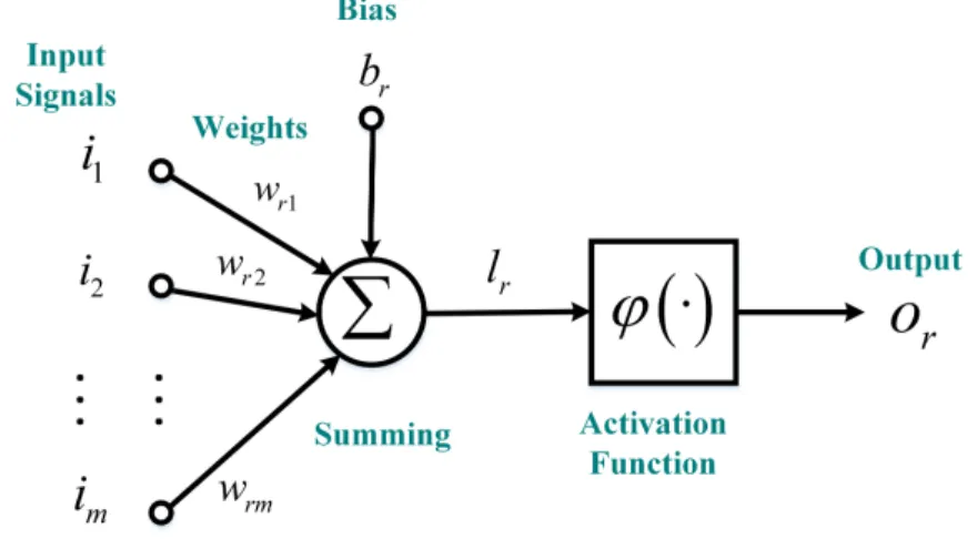
A neuron is an information processing unit which is fundamental to the operation of a neural network. Figure 2.2 shows the model of a neuron. We call this neuron neuronr since a neural network is constructed by many neurons (see Figure 2.4 and Figure 2.5 in Section 2.2.2). In Figure 2.2, neuronrtakes several signals, namely,i1,i2, ...,im
1) A set of connecting links. Each of these links is characterized by a weightwrj,
j∈[1, m]. An input signalijis connected to neuronrby multiplying the weightwrj; 2) An adder. This adder sums the input signals (i1,i2, ...,im), weighted by the corresponding weights mentioned above;
3) An activation function. This activation function limits the amplitude of the output signalorto be in a certain range. Typically, the range of the output of a neuron is limited to[0,1]or[−1,1].
Figure 2.2: The model of a neuron.
Figure 2.2 shows that the model of a neuron also includes an externally applied parameter called bias. The bias is denoted bybrin this model of neuronr. The bias
bris used to increase or decrease the input of the activation function.
In mathematical terms, we can model neuronrby using Equations (2.2), (2.3) and (2.4), wherei1,i2, ...,imare the input signals to neuronr;wr1,wr2, ...,wrmare the weights of neuronr;bris the bias;ϕ(·)is the activation function; andoris the output of neuronr.
ur= m X
j=1
wrjij (2.2)
lr=ur+br (2.3)
2.2.1.2 Types of Activation Functions
The aforementioned activation function, denoted byϕ(·), defines the output of neuron
r. Here, we introduce some basic activation functions:
1) Threshold Function. The threshold function is given by Equation (2.5), where
ϕ(·)denotes the activation function; andlrdenotes the input to the activation function
ϕ(·), andlris defined using Equation (2.3).
ϕ(lr) =
1 if lr≥0
0 if lr<0
(2.5)
2) Sigmoid Function. The sigmoid activation function is given by Equation (2.6), whereais used to control the output of the sigmoid function. Note that the output of a sigmoid function is in a continuous range[0,1]while the output of the threshold function is ether 1 or 0.
ϕ(lr) =
1
1 +exp(−alr) (2.6)
3) Rectified Linear Unit (ReLU) Function. The ReLU function is given by Equa-tion (2.7). ReLU is by far the most commonly used activaEqua-tion funcEqua-tion in CNNs.
ϕ(lr) =max(0, lr) (2.7) 4) Softmax Function. The Softmax function is given by Equation (2.8), wherep denotes that there arepneurons in total in a layer of a neural network. The layer of a neural network is described in Section 2.2.2.
ϕ(lr) =
elr
Pp n=1eln
(2.8)
2.2.2 The Architecture of a Neural Network
Figure 2.3: Architectural graph to model a neuron.
...,imand an outputor. How neuronrworks in this graph is given by Equations (2.2), (2.3) and (2.4) (For details please see Section 2.2.1.1).
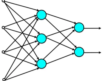
In a neural network, the neurons are organized in the form of layers. In the simplest form of a neural network, we have an input layer of input signals that projects onto an output layer of neurons. We call this neural network the single-layer neural network. Here "single-layer" refers to the output layer of the network. We do not count the input layer of this network because there is no computation performed in the input layer. Figure 2.4 shows an example of a single-layer neural network. In this example, this single-layer neural network has four input signals and has one output layer of two neurons that produce outputs.
preceding layer only. The neural network shown in Figure 2.5 is also called a fully-connected neural network in the sense that every node in each layer of the network is connected to every other node in the adjacent forward layer. Here a node denotes an input signal or a neuron in the graph shown in this figure.
Figure 2.4: An example of a single-layer neural network.
2.2.3 Learning Process of a Neural Network
As discussed in Section 2.1, when we use a neural network as a machine learning model, we need to use a learning algorithm to find a set of parameters, i.e., the weights and biases of all neurons in the neural network, that make this neural network be able to map inputXto labelyin the training dataset. However, the learning algorithm is not able to calculate the perfect weights and biases for a neural network. Instead, the learning process of a neural network is regarded as an optimization problem, where the learning algorithm is used to explore the space of possible sets of weights and biases for the neural network. We use a function to evaluate a candidate solution (i.e. a set of weights and biases for the neural network). This function is called a cost function or a loss function. For example, we can define a cost function as given in Equation (2.9). In this equation,X denotes the input vector in the training dataset andX(i)is theith input feature vector in the training dataset. y denotes the desired output of the network andy(i)is the desired output of the network when the input to the network isX(i).fN N(·)denotes the neural network. W denotes all the weights in the neural network.Bdenotes all the biases in the network. Fdenotes the total number of input feature vectors. This loss function is called the Mean Squared Error (MSE) cost function. From this cost function, we can see thatC(W, B)is non-negative. When the costC(W, B)becomes very small, i.e.,C(W, B)is close to 0,fN N(X, W, B)is approximately equal toy. This means that the learning algorithm has found very good weightsW and biasesB such that the neural network with these weights and biases approximately maps the input of this networkXto the desired output of the network
y. In contrast, when the costC(W, B)is large, this means thatfN N(X, W, B)is not equal toy, showing that our neural network with the weights W and the biasesB cannot map well the input of this networkXto the output of the networky. Now, the cost function that is commonly-used for a neural network is called the cross-entropy cost function. The cross-entropy cost function is given in Equation (2.10). In this equation,Edenotes that there areEneurons in the output layer of a neural network.
y(ji)denotes the desired output of thejth neuron in the output layer of a neural network when the input to the network isX(i). fN Nj(X
(i), W, B)
denotes the actual output of thejth neuron in the output layer of a neural network when the input to the network isX(i).
C(W, B) = 1
F
F X
i=1
ky(i)−fN N(X(i), W, B)k2 (2.9)
C(W, B) =−1
F F X i=1 E X j=1
[yj(i)log(fN Nj(X
(i), W, B)) + (1−y(i)
j )log(1−fN Nj(X
(i), W, B))]
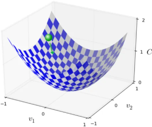
From the aforementioned description, we can see that the objective of the learning algorithm is to minimize the costC(W, B). More specifically, we seek to find a set of weightsW and biasesB that minimize this cost as much as possible. For better readability, we useC(v) to denote a cost function. C(v)can be a function of many parameters such asv =v1, v2, ...,vh. SupposeC is a function of just two parame-tersv1,v2. Figure 2.6 shows an example of functionC withv1 andv2. Our object is to findv1, v2 whereC achieves its minimum. For the simple function shown in Figure 2.6, we can use calculus to try to find the minimum analytically. We could compute derivatives and then try using them to find places where C is an extremum. However, the cost function of a neural network can have many more parameters and be much more complex because a neural network contains much more parameters, i.e., the weights and biases of all neurons in the network. For example, very large neural networks have cost functions that depend on billions of weights and biases. It is impossible to use calculus to minimize the cost function.
direction and a small amount4v2 in thev2 direction by using Equation (2.11). We need to find4v1and4v2that make4Cnegative (negative4Cmeans that the ball is rolling down into the valley). We define that4vis equal to(4v1,4v2)T as shown in Equation (2.12), whereTis the transpose operation that turns row vectors into column vectors in a matrix. We define that the gradient ofC, denoted by5C, is equal to the vector of partial derivatives (∂v∂C1,
∂C ∂v2)
T
, as shown in Equation (2.13). With these definitions, Equation (2.11) can be rewritten to be Equation (2.14). In order to make
4Cnegative, we can make4vto be equal to−η5Cas shown in Equation (2.15), whereη is a small, positive parameter, called the learning rate. Then, by combing Equation (2.14) and Equation (2.15),4C=−η5C· 5C=−ηk 5Ck2. Because
k 5Ck2 ≥0
andη >0,4C ≤0. This means thatCwill always decrease and never increase. Thus, we use Equation (2.15) to define the rule of how to move the ball in the gradient descent algorithm. This means that we use Equation (2.15) to compute a value4vand then move the position of the ballvto a new positionv0by the amount of4v, as shown in Equation (2.16). Then we will use updated rule again to make another movement of the ball. By keeping doing this, we can decreaseC until we reach the (approximate) minimum of the cost functionC.
Figure 2.7: The analogy of using gradient descent to minimize a cost function.
4C≈ ∂C
∂v1
4v1+
∂C ∂v2
4v= (4v1,4v2)T (2.12)
5C = (∂C
∂v1
, ∂C ∂v2
)T (2.13)
4C ≈ 5C· 4v (2.14)
4v =−η5C (2.15)
v→v0=v−η5C (2.16)
The aforementioned discussion describes how the gradient descent method works when the cost functionChas two parameters. WhenCis a function ofhparameters, i.e.,v1,v2, ...,vh,5Cis calculated using Equation (2.17). We repeatedly apply the rule shown in Equation (2.18) until we reach the (approximate) minimum of the cost functionC.
5C= (∂C
∂v1
,∂C ∂v2
, ..., ∂C ∂vh
)T (2.17)
v→v0=v−η5C (2.18)
5CW = (
∂C ∂w1
, ∂C ∂w2
, ..., ∂C ∂wd
)T (2.19)
W →W0 =W −η5CW (2.20)
5CB= (
∂C ∂b1
,∂C ∂b2
, ...,∂C ∂bg
)T (2.21)
B →B0=B−η5CB (2.22)
Now, researchers often use the gradient descent method with momentum, which is called the momentum-based gradient descent method. The momentum technique modifies the gradient descent method in two ways. Firstly, the momentum technique introduces a notion of “velocity” for the parameters we optimize. The gradient descent method changes the “velocity” of the parameters, not (directly) the “position” of the parameters, and only indirectly affects the “position” of the parameters. Secondly, the momentum technique introduces a friction term, which can gradually reduce the “velocity” of the parameters. In mathematical terms, the momentum-based gradient descent method replaces the updating rule forW (given in Equation (2.20) used in the gradient descent method without momentum) with a new updating rule given in Equation (2.23), and (2.24), whereVwdenotes the aforementioned “velocity” forW, andµdenotes the aforementioned friction term and is called the momentum param-eter. Also, the momentum-based gradient descent method replaces the updating rule forB(given in Equation (2.22) used in the gradient descent method without momen-tum) with a new updating rule given in Equation (2.25), and (2.26), whereVbdenotes the aforementioned “velocity” forB.
Vw →Vw0 =µVw−η5CW (2.23)
W →W0=W +Vw0 (2.24)
B →B0 =B+Vb0 (2.26) One problem of the learning process of a neural network is called overfitting. Overfitting happens when a neural network learns the details of the training data to the extent that it negatively impacts the performance of this neural network on new data. This means that random fluctuations in the training data is learned by the neural network. Unfortunately, the learned random fluctuations cannot apply on new data, thereby negatively impacting the generalizing ability of the network.
In order to reduce the overfitting, one commonly-used technique, called weight decay, is utilized. The weigh decay technique modifies the updating rule for weights
W and does not change the updating rule for biasesBin the gradient descent method. The gradient descent method with weight decay replace the updating rule forW (given in Equation (2.20) used in the gradient descent method without weight decay) with a new updating rule given in Equation (2.27). In Equation (2.27), λ is called the weight decay parameter;F denotes the total number of input feature vectors andηis the learning rate. The updating rule forB used in the gradient descent method with weight decay is the same as the updating rule forB (given in Equation (2.22)) used in the gradient descent method without weight decay.
W →W0 = (1− ηλ
F )W −η5CW (2.27)
2.3
Convolutional Neural Network
Convolutional Neural Network (CNN) is a specific kind of neural network. In re-cent years, CNNs have been the most commonly-used neural networks to recognize images.
a tensor and denotes the inputs to the neural network. For example, ifXis an image with 640×480 pixels, we callXa (640×480) tensor. We train this neural network
fN N(·)with the training dataset that consists of handwritten digits with their corre-sponding labels (e.g., 1, 3, 6). As introduced in Section 2.2.3, the gradient descent is used to find the weightsW and biasesBthat make the neural networkfN N(X, W, B)
build the (approximate) mapping from the handwritten digits to the labels. Then, for a new handwritten digit, the trained neural network can predict a label for this new handwritten digit.
Up to this point, we have known how to use a neural network to recognize images of handwritten digits. Now let us introduce the reason of why the fully-connected neural network has the problem of using a large number of parameters to recognize images. In the aforementioned example of the handwritten digit recognition, the input is an image of a handwritten digit. This image is 28×28 pixel image. This means that the number of the input signals in the input layer of a fully-connected neural network is 784 = 28×28. Suppose a simple fully-connected neural network which architec-ture is a 2-layer network with one hidden layers and one output layer. We suppose that each hidden layer has 10 neurons and the output layer of this neural network has 10 neurons. The number of parameters (i.e., all weights and biases) of this neural network is (784×10+10) + (10×10 + 10) = 7960. Unfortunately, such simple fully-connected neural network cannot work well to recognize handwritten digits. Suppose a more complex fully-connected neural network which architecture is a 3-layer net-work with two hidden layers and one output layer. Each hidden layer of this netnet-work has 50 neurons, and the output layer still has 10 neurons. The number of parameters of this network is 42290. From this example, we can see that with the increase of the number of hidden neurons and hidden layers, the number of the parameters of a fully-connected layer is dramatically increased. This means that when we design a fully-connected neural network that can be useful for image recognition, the number of the parameters of such network will be large. The large number of parameters dra-matically increases the time of training such fully-connected neural network because in the training process, the gradient descent algorithm will need quite a long time to find a large number of parameters that make this network (approximately) maps the handwritten digits to the labels (For details of the training process of a neural network, please see Section 2.2.3).
2.3.1 The Convolution Operation
The convolution operation is an important operation in analytical mathematics. In this section, we introduce the 2-dimension convolution operation because the 2-dimension convolution operation is widely used for image recognition and also used in our pro-posed CNN-based methods for P300-based BCIs in this dissertation.
The 2-dimension convolution operation is defined by Equation (2.28), where⊗ denotes the convolution operation.Z,X, andKare 2-dimension matrices.Xdenotes the input matrix to the convolution operation;Zdenotes the outputs of the convolution operation;K is called the kernel of the convolution operation. (k1,k2) is called the kernel size. (s1,s2) is called the stride. In Equation (2.28),Z(i, j)denotes the datum in theith row and thejth column of the matrixZ;X(i, j)denotes the datum in the
ith row and thejth column of the matrixX; andK(m, n)denotes the datum in the
mth row and thenth column of the matrixK.
Z(i, j) = (X⊗K)(i, j) =
k1−1
X
m=0
k2−1
X
n=0
X((i−1)s1+ 1 +m,(j−1)s2+ 1 +n)K(m, n)
(2.28)
2.3.2 The Characteristics of Convolutional Neural Network
to connect to the second hidden neuron in the first hidden layer. For each receptive field, there is a corresponding hidden neuron connected with this receptive field in the hidden layer. In this way, we build a hidden layer, and this hidden layer is called a feature map.
2) Parameter Sharing. Secondly, we introduce the parameter sharing in the CNN. Here, the parameter denotes the weights and biases used in a CNN. As described above, each hidden neuron in the hidden layer uses one biases and some wights that are connected to the corresponding receptive field. The parameter sharing means that all the neurons in a hidden layer of a CNN use the same weights and bias. The char-acteristic of parameter sharing in CNN is able to significantly reduce the number of parameters. Thus, the parameter sharing can solve the problem in the fully-connected neural networks, i.e., the fully-connected neural networks use a large number of pa-rameters when used to recognize a image.
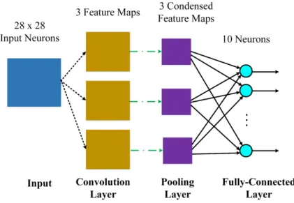
3)Pooling Layers. Finally, we introduce the pooling layers in the CNN. Pooling layers are often used after the convolution layers. The pooling operation in a pooling layer converts each feature map from the convolution layer into a condensed feature map by summarizing a region of neurons in the feature map. For example, the pooling operation, called max-pooling, takes the maximum in a region of neurons as a unit in the pooling layer. A CNN often uses more than one feature map, and the pooling operation is applied to each feature map, separately. Thus, if there are 5 feature maps, the pooling layer will output 5 condensed feature maps.
2.3.3 The Architecture of Convolutional Neural Network
Figure 2.8: An example of the architecture of a CNN used for the handwritten digit recognition.
2.4
P300-based Brain Computer Interface
In this dissertation, we focus on P300-based BCIs. The P300 signal is the target sig-nal used in a P300-based BCI and the P300 speller is the benchmark and the most commonly-used application of a P300-based BCI. First, we introduce some back-ground information on the P300 signal and the P300 speller in Section 2.4.1 and Sec-tion 2.4.2, respectively. Then, we describe the metrics to assess the performance of the P300 speller in Section 2.4.3.
2.4.1 P300 Signal
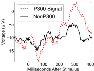
Figure 2.9: P300 signal.
The subject in this paradigm is detecting a rare target stimulus among the non-target stimuli. The P300 signal is only able to be evoked in the subject’s brain when this subject detects the rare target stimulus.
The P300 signal is typically measured most strongly by the electrodes covering the parietal lobe. The amplitude of a P300 signal varies with the rareness of the target stimulus. The latency of a P300 signal varies with the difficulty of discriminating the target stimulus from the non-target stimuli. For example, the typical latency of a P300 signal evoked in a young healthy adult is about 300ms while the latency of a P300 signal evoked in subjects (persons) with decreased cognitive ability is longer than 300ms. Due to its reproducibility and ubiquity, the P300 signal is a common choice for psychological tests in both the clinic and laboratory.
of not having a P300 signal in this time period.
E(X) =
1 if P1 > P0
0 otherwise (2.29)
2.4.2 P300 Speller
Farwell and Donchin developed the first P300-based BCI character speller in 1988 [FD88]. The subject in the experiment is presented with a 6 by 6 character matrix (see Figure 2.10) and he focuses his attention on a target character he wants to spell. All rows and columns in this matrix are intensified successively and randomly but separately. Each row or column intensification lasts for time periodt1, followed by a blank time period of the matrixt2. Two out of twelve intensifications contain the target character, i.e., one target row and one target column. As a result, the target row/column intensification becomes a rare stimulus to the subject. A P300 signal is then evoked by this rare stimulus. By detecting the P300 signal, we can infer which row or column the subject is focused on. By combing the row and column positions, we can infer the target character position. After the inference of one character, the matrix is blank for time periodt3 to inform the subject that the current character is completed and to focus on the next character.
Figure 2.10: P300 speller character matrix.
result, in practice, experimenters use many epochs to help the subject spell one char-acter. The detailed calculation for determining the position of the target character is given in Equations (2.30), (2.31), and (2.32), whereP(1i,j)denotes the probability of
the presence of a P300 signal in the jth intensification and the ith epoch, Sum(j)
denotes the sum of the probabilities for thejth intensification when usingkepochs,
indexcoldenotes the column index of the target character in the matrix in Figure 2.10, andindexrow denotes the row index of the target character. Whenj ∈ [1,6],j de-notes a column intensification. Whenj ∈ [7,12], j denotes a row intensification. Equation (2.30) cumulates the probabilities of having a P300 signal evoked by inten-sificationjoverkepochs. In Equation (2.31), we assign the index of the maximum
Sum(j) toindexcol when j ∈ [1,6]. This equation finds the index of the column intensification, with the maximum sum of probabilities, to have evoked a P300 sig-nal. This index is the column position of the target character when usingkepochs. In Equation (2.32), the row position of the target character when usingkepochs is calculated in the same way as in Equation (2.31). The position of the target character in the matrix in Figure 2.10 is the coordinate formed by the target row position and the target column position.
Sum(j) = k X
i=1
P(1i,j) (2.30)
indexcol =argmax 1≤j≤6
{Sum(j)} (2.31)
indexrow =argmax 7≤j≤12
{Sum(j)}
(2.32)
2.4.3 Performance Assessment of P300 Speller
As indicated in Chapter 1, in this dissertation, we use the P300 speller as the bench-mark application of a P300-based BCI. As the benchbench-mark application of a P300-based BCI, we need metrics to assess the performance of the P300 speller. More specifically, we need metrics to assess the communication accuracy and the communication speed of the P300 speller. As typically done in related research works for the P300 speller, we use the character spelling accuracy to assess the communication accuracy of the P300 speller as well as we use the Information Transfer Rate (ITR) to assess the com-munication speed of the P300 speller.
To calculate the character spelling accuracy of the P300 speller, we use Equa-tion (2.33). In this equaEqua-tion,accchar(k)denotes the character spelling accuracy when
correctly inferred characters when usingkepochs for each character, andScdenotes the number of all characters.
accchar(k)= Ntc(k)
Sc
(2.33)
In addition to using the character spelling accuracy to assess the communication accuracy of the P300 speller, we also use the Information Transfer Rate (ITR) for the assessment of the communication speed of the P300 speller. ITR has been the most commonly applied metric to assess the communication speed of P300-based BCIs [WW12, LWG16, NRS17, IKV18]. ITR has been introduced by Shannon and Weaver [SW49]. It is calculated by Equation (2.34) [WRMP98], whereaccchar(k)is calculated using Equation (2.33) andNclais the number of classes. Here, we have 36 characters to spell (see Figure 2.10), soNcla=36.Tkdenotes the time needed to spell a character when usingkepochs. Tk is calculated using Equation (2.35), wheret1,
t2, andt3 are the time periods described in the first paragraph of Section 2.4.2. For more detailed explanation of Equation (2.34), please refer to [WRMP98].
IT Rk=
60(accchar(k)log2(accchar(k)) + (1−accchar(k)) log2(
1−accchar(k)
Ncla−1 ) + log2(Ncla)) Tk
(2.34)
Tk=t3+ 12×(t1+t2)×k 1≤k≤15 (2.35) Here, we calculate the theoretical maximum ITR when the datasets described in Section 2.5 are used in this dissertation because we want to compare the ITR achieved by our methods with the theoretical maximum ITR. When using the datasets described in Section 2.5,Ncla=36,t1=100ms,t2=75ms, andt3=2.5s (for details please refer to Section 2.5). The theoretical maximum ITR is achieved when we use the least time to spell a character and achieve the highest spelling accuracy. The least time to spell a character means that we use only one epoch to spell a character. i.e.,k=1. Thus, the least time we use to spell a character isT1= 2.5s + 12×(0.1s+0.075s) = 4.6s. The highest spelling accuracy is 100% (i.e.,accchar(1) = 1). As a result, the theoretical
maximum ITR when using the datasets described in Section 2.5 is 60 log4.26(36)bits/min = 67.43 bits/min.