T-CYCLE EPR Development at 275 GHz for the study of reaction kinetics & intermediates

(1)

The handle

http://hdl.handle.net/1887/68233

ho

lds various files of this Leiden University

dissertation.

Author: Panarelli, E.G.

Title:

T-CYCLE EPR Development at 275 GHz for the study of reaction kinetics &

intermediates

(2)

T-CYCLE EPR

Development at 275 GHz for the study

of reaction kinetics & intermediates.

Proefschrift

ter verkrijging van

de graad van Doctor aan de Universiteit Leiden,

op gezag van Rector Magnificus prof.mr. C.J.J.M. Stolker,

volgens besluit van het College voor Promoties

te verdedigen op maandag 10 december 2018

klokke 16.15 uur

door

Enzo Gabriele Panarelli

geboren te Cuneo (Itali¨e)

(3)

Co-promotor: Dr. P. Gast

Promotiecommissie: Prof. dr. W. J. Buma (Universiteit van Amsterdam)

Prof. dr. E. Giamello (Universit`a di Torino, Turijn, Itali¨e)

Prof. dr. H. J. Steinhoff (Universität Osnabrück, Osnabrück, Duitsland)

Prof. dr. E. R. Eliel

Prof. dr. M. A. G. J. Orrit

Casimir PhD series, Delft-Leiden 2018-43

ISBN 978-90-85933731

An electronic version of this thesis can be found at https://openaccess.leidenuniv.nl

(4)

(5)

(6)

A−−→k1 I−−→k2 P, with A being the reagent (plotted in red), I the intermediate (plotted in green), and P the product (plotted in blue). Notice that in this example no equilibrium is considerered in between the elementary reactions. Furthermore, the second elementary reaction, generating the product from the intermediate, is faster than the first elementary reaction, beingk2= 5k1.

1.3 Rapid Freeze-Quench

One of the most commonly used techniques to trap reaction intermediates on time scales of

milliseconds is the so-called Rapid Freeze-Quench (RFQ), first implemented by Bray in 1961 [18]

and in use ever since. Owing to the relatively high time resolution of this technique (down to

mil-liseconds), and to the possibility to couple it to several spectroscopic detection methods, RFQ has

(16)

1. INTRODUCTION

Resonance (EPR). Chapter 2 of this thesis is devoted to the coupling of RFQ to high-frequency

EPR, and many details are provided there. Here, a brief introduction to the principles of RFQ is

provided.

RFQ consists of the rapid reaction quench of a mixture of two or more chemically reactive

samples, caused by the mixture’s fast freezing in a cryogenic bath. Prior to the freezing, the

reagents have first rapidly and homogeneously mixed and then reacted for a well-defined amount

of time. In the setup used for the experiments of Chapter 2 of this thesis, the two reactants (here

labeled A and B) are contained in two separate syringes that are mounted on a stage coupled

to a ram. The ram is connected to a console-controlled servo motor that can move the ram

upwards, thereby pushing the pistons of the syringes symmetrically and injecting equal volumes

of the solutions of reactants to the mixer, to which the syringes are connected by suitable plastic

tubes. The mixer is specifically designed to rapidly and homogeneously mix the two reactant

solutions before injecting them to a so-calledaging tube, whose length is one of the parameters

that determine the reaction time (tr) of the mixture. At the end of the aging tube is a nozzle

that sprays the mixture into a cryogenic bath (most commonly isopentane at a temperature of

about 140 K). The cold medium immediately freezes the droplets of mixture, thereby quenching

the reaction at a specifictr. The frozen droplets take the shape of particles that can be collected

in a sample holder for later measurements. Specifically in this thesis (see Chapter 2), the RFQ

particles were collected in EPR tubes and later transferred into smaller capillaries suitable for

high-frequency EPR.

In the RFQ setup used in Chapter 2, three parameters can be directly set in the ram-controlling

console, which will determine the reaction time of the mixture for a given length of the aging tube. These parameters are:

• theram velocity UR (between 0.8 and 8 cm s−1), which is the actual velocity of the ram;

• thetotal displacement dT (between 0.01 and 10 cm per experiment), which is the length

by which the ram moves per experiment;

• the delay factor, which sets one or more incubation times between consecutive ram dis-placements.

For the RFQ experiment designed in Chapter 2, only the first two settings were taken into

account. In what follows is shown how the ram velocity and the total displacement directly affect

(17)

aging tube. The flow rate in turn affects the reaction time, which is the time the mixture spends

in the aging tube, and thus the time amount by which the reaction has progressed. Notice that

the following equations were derived from [19], whose notation is reproduced here.

The flow rate (in mL s−1) is described by the continuity equation relating the ram velocity

(directly set from the console) and the flow velocity in the aging tube:

Q=AsUR=ArUx (1.9)

where As is the cross-sectional area of the syringe (in cm2),UR is the ram velocity (in cm

s−1_), _A

r is the cross-sectional area of the aging tube (in cm2), and Ux is the flow velocity in

the aging tube (in cm s−1). Since the cross-sectional area of the syringe is related to the total

volume of the syringe, being Vs =AsdT, it results from Equation 1.9 that Q= _dVs

TUR, which indicates that the flow rate is directly determined by the console-controlled ram velocity and

total displacement.

Since the flow velocity in the aging tube can be expressed asUx=lr/tr, the numerator being

the length of the aging tube and the denominator being the time the mixture spends in the

reaction tube (or reaction time), through Equation 1.9 it is possible to express the reaction time

as:

tr= lr Ux

=Ar As lr UR = _D r Ds 2 _l r UR (1.10)

where Dr and Ds are the diameters of the aging tube and of the syringe, respectively. In

the experiments described in Chapter 2 of this thesis, they have values of 0.05 cm and 0.7 cm,

respectively, while the ram velocity is set to 3.2 cm s−1. In this way, once the console parameters

are set, and the syringe volume and the aging tube diameter are known, Equation 1.10 allows

to calculate the reaction time per RFQ experiment only as a function of the length of the aging

tube.

A final important remark concerns the so-called dead time or – as is called in Chapter 2 – thefreezing timeof the RFQ setup. Owing to the connections between the tubes, the syringes,

and the mixer, any RFQ setup has an intrinsicdead volume that is filled by the mixture during the freezing time, which adds up to the actual reaction time. The temporal outcome of a RFQ

experiment is thus expressed in terms of an overall non-consistently definedaging time [20] or

(18)

1. INTRODUCTION

1.4 Laser-induced Temperature-jumps

The laser-induced Temperature-jump (T-jump) methodology was originally developed to study

the relaxation of (bio)chemical systems in equilibrium, following the perturbation of the

equi-librium induced by a heat source (such as an electrical discharge [22] or a near-infrared (NIR)

laser pulse [23]), which causes the system to quickly reach a higher temperature before going

back to the initial temperature after the heat source is turned off. Particularly in the case of a

laser-induced T-jump, the absorption of the NIR energy, typically by the solvent molecules (e.g.,

water), results in the heating of the sample volume, with a temperature difference (∆T) that

depends on:

• the heat conductivity and heat capacity of the solvent and sample holder; • the optical intensity of the laser pulse;

• the optical absorption of the solvent molecules at a specific excitation wavelength.

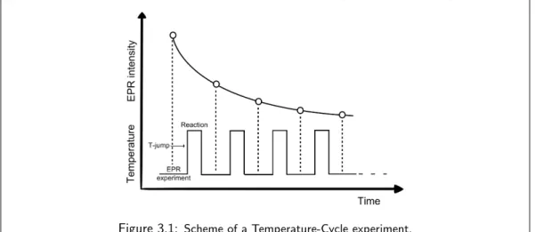
In this thesis, a laser-induced T-jump methodology was developed, in combination with

high-frequency Electron Paramagnetic Resonance (hence named T-Cycle EPR), for the investigation

of reaction kinetics between two chemically reactive species. The T-jump method developed here

has similarities with the one employed for relaxation studies. However, the important difference

with T-jump relaxation methodologies is that T-Cycle EPR involves the application of T-jumps

on a system that does not feature any chemical equilibrium, i.e., a frozen mixture of reactants

where no reaction is taking place. As such, the method is thus not developed with the aim of

observing the relaxation of the system back to its equilibrium state following a laser-induced

T-jump. Rather, the jumps applied here serve as ”heating shots” that warm up the system to

a temperature where a chemical reaction can take place for a certain amount of time, to which

follows the return of the system to a frozen state where no reaction occurs. This allows the

observation of the step-wise progress of a chemical reaction as a function of time, with no focus

whatsoever as regards the relaxation of the system.

An important aspect of the sample heating with a laser pulse for kinetic studies is that it

should take place homogeneously over the whole sample volume, so as to ensure a single,

well-defined reaction temperature of the sample – this being the equilibrium temperature between two

opposing driving forces, namely the heating by the laser pulse, and the cooling by the thermal

bath. To this end, a small sample volume is paramount, in order to maximize the rate of heat

(19)

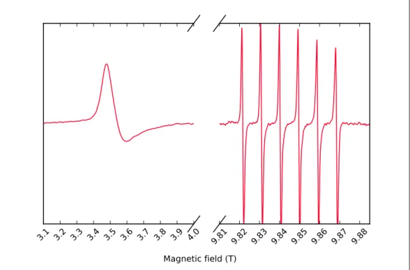
to high-frequency EPR, which makes use of relatively small sample volumes. Evidence of the

homogenous heating produced by the laser pulses used in the setup of T-Cycle EPR described in

this thesis is given in Figure 1.2, where the 275 GHz cw EPR spectra of a solution of TEMPOL

in a mixture of water and glycerol are shown as a function of the nominal laser power. To

record these spectra, the laser was turned on continuously, and a spectrum was recorded for

different laser powers, in increasing order. These spectra can be easily interpreted and simulated

by taking into account one single spectral component (as described in the Appendix to Chapter

3), which implies they are not the summation of many different spectra that originate from zones

of the sample at different temperatures. The homogenous heating of the sample produced by

the laser-induced T-jumps applied here is facilitated by the small sample volume (about 20 nL),

and is in agreement with what has been reported by Azarkh and Groenen in [24].

A key point to achieve fast and homogenous T-jumps is the efficient absorption of the NIR

energy by the solvent molecules. Water has a broad absorption in its NIR spectrum peaking

around 1450 nm, originating from the first overtone of the O—H bond stretching [25]. The

absorption coefficients at 1600 nm (i.e., about the wavelength of the laser used in Chapters 3

to 5, at 1550 nm) of pure water [26], pure glycerol [27], and mixtures of water and glycerol

1:1 in volume [27] are, respectively, 7.7, 11.6, and 9.8 cm−1. In particular, the mixture of water

and glycerol has an absorption increased by roughly 25% as compared to that of pure water, an

observation in agreement with the work by Azarkh and Groenen [24].

1.5 Electron Paramagnetic Resonance

Electron Paramagnetic Resonance (EPR) is a powerful spectroscopic technique useful for

struc-tural investigations of paramagnetic species such as organic radicals, metal ions, or defect centres

in solids. Similarly to the more common Nuclear Magnetic Resonance (NMR), where

radio-frequency-induced nuclear spin transitions are measured, in EPR microwave-induced transitions

between electron spin energy levels are detected. Since the energy of the spin levels of an electron

are very sensitively influenced by its environment, valuable information can be extracted from

an EPR spectrum when the quantum mechanical energy description of the electron – its spin

Hamiltonian – is known. Nowadays, alongside the traditional continuous-wave (cw) approach in

EPR, more and more sophisticated microwave pulse sequences are being developed to provide

ever more detailed information on the spin systems of interest. Moreover, the technical

achieve-ments in microwave technology made EPR at higher microwave frequencies feasible, making it

very accessible and widespread, allowing improved spectral resolution (both in EPR and

(20)

1. INTRODUCTION

9.80 9.81 9.82 9.83 9.84 9.85

Magnetic field (T)

Figure 1.2: 275 GHz cw EPR spectra of TEMPOL, at a concentration of 1 mM, in solution with

a mixture of water and glycerol 95:5 in volume. The spectra are recorded with the laser turned on continuously at increasing optical power (top blue @ 0.0 W, bottom red @ 2.0 W), from a cryostat temperature of -50°C.

spin Hamiltonian (like the zero-field splitting), and a higher absolute sensitivity owing to a large

Boltzmann factor [12], not to mention that in certain systems the only possibility to induce EPR

transitions is with microwave quanta of high frequency. Hereinafter is a general introduction to

the basic theory of EPR meant to understand the spin systems studied in this thesis. Complete

treatments of the subject can be found, for instance, in [28] and [29].

1.5.1 The electron Zeeman effect and the

g

-factor

To illustrate the principles of EPR, the simplest paramagnetic system is considered first, namely

an isolated electron having a spinS=1_/_{2. When a particle with non-zero spin is subject to an}

externally applied magnetic field, the energy levels associated to its spin will split as a function of

the magnetic field (Equation 1.11), a phenomenon first observed by the Dutch physicist Pieter

Zeeman and thus called Zeeman effect. Quantum mechanically, energy levels resulting from such

(21)

H=geµBS·B (1.11)

where ge = 2.0023 is the g-factor of an isolated electron in the vacuum, µB is the Bohr

magneton,Bis the external magnetic field, andSis the electron spin. SinceBis oriented along

one direction (conventionally, z), only the magnetic field magnitude B0 is taken into account,

and therefore only theSzcomponent of the spin operatorS. In particular for the case ofS=1/2,

the eigenvalues ofSz aremS =±1₂, and the eigenvalues of the spin Hamiltonian of Equation

1.11 (namely, the energy levels of the electron spin) can be written asE±=±12geµBB0, which

evidences the dependence of the energy splitting on the external magnetic field.

The energy splitting of the spin levels is thus proportional to the magnitude of the external

magnetic field, but also depends on theg-factor, a quantity that acts as a proportionality constant

and is very sensitive to the magnetic environment of the electrons. In general, theg-factor is a

tensorial entity,g, and is calledanisotropicwhen the diagonal componentsgx,gy, andgzof the

matrix representation in the eigenbasis of gare not equal. When this is the case, the splitting

of the spin levels is different in different spatial directions, and the EPR transition arising from

the spin Hamiltonian of Equation 1.11 will be observed at different values of the magnetic field,

each one associated to a direction ofg.

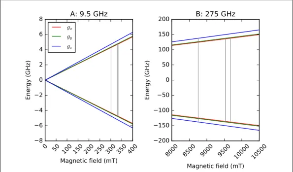
To better illustrate the Zeeman effect and the influence of an anisotropic g-factor, in Figure

1.3 are plotted the spin levels of an S = 1_/₂ _{system with a strongly anisotropic} _g _{(as is the}

case for the system described in Chapter 5 of this thesis) as a function of the externally applied

magnetic field. At zero field, the spin states are degenerate, and by increasing the magnitude of

the external magnetic field, such states are split anisotropically and proportionally to gx (red),

gy (green), orgz (blue). When operating at 9.5 GHz (Figure 1.3 A), one of the most common

frequencies in EPR, the three transitions (depicted as grey lines) associated to the three different

values ofgare observed between roughly 300 and 350 mT. In particular, the two at higher field

(corresponding to gx and gy) are separated by about 5 mT. When going to higher magnetic

field, a correspondingly higher microwave frequency is required to match the energy difference

between the spin levels and induce an EPR transition. Figure 1.3 B shows such situation at the

EPR frequency of 275 GHz, with the three transitions associated to the anisotropicgspreading

between about 8700 and 9600 mT, and the two at higher field separated by about 140 mT. This

simple example highlights a fundamental advantage of high-frequency (HF) EPR versus

low-frequency (LF) EPR, namely a better resolution in magnetic field even for slightly anisotropic

(22)

1. INTRODUCTION

0 50 100 150 200 250 300 350 400

Magnetic field (mT)

−8

−6

−4

−2

0

2

4

6

8 En

e g

y (

GHz

)

A: 9.5 GHz

gx

gy

gz

800

0

850

0

900

0

950

0 ₁₀₀

00 ₁₀₅

00 Magnetic field (mT)

−200

−150

−100

−50

0

50

100

150

200 En

e g

y (

GHz

)

B: 275 GHz

Figure 1.3: Simulated electron spin energy levels for anS=1_/₂_{system with anisotropic}_g_(whose

x, y, and z components are represented in red, green, and blue, respectively), subjected to the Zeeman effect in the presence of an external magnetic field. (A) EPR transitions at the microwave frequency of 9.5 GHz (gray lines). (B) EPR transitions at the microwave frequency of 275 GHz (gray lines). The g-valuesgx = 2.037, gy = 2.067, and gz = 2.25 are from [30]. Any other effect apart from the electron Zeeman is not included in the simulations, which are performed with EasySpin [31].

1.5.2 Electron spin – nuclear spin interaction: the hyperfine coupling

One of the most interesting properties of spins is their ability to interact with each other. The

interaction between electron spins and nuclear spins, called hyperfine coupling, provides a great

deal of information about the chemical environment of an electron. In the general case where one

electron with spinS =1_/₂_{interacts with one nucleus with spin}_I_{, the resulting spin Hamiltonian}

can be expressed as:

H=geµBS·B−gNµNI·B+S·A·I (1.12)

where the first term represents the electron Zeeman effect, the second term represents the

(23)

electron spin and the nuclear spin. Like for the electron Zeeman term, also the nuclear Zeeman

term contains a nuclearg-factor,gN, and the nuclear magneton,µN. The hyperfine interaction

is represented by the tensor A, which can be viewed as composed of anisotropic contribution and ananisotropicone (similarly to thegtensor), namely A=aiso+T.

The effect of the Zeeman term on the nuclear spin is similar to that on the electron spin,

namely it splits the energy levels of the nuclear spin as a function of the external magnetic

field. To understand how this works, Figure 1.4 schematically illustrates the energy splitting of

a system composed of one electron spin S = 1_/₂ _{with isotropic} _g_{-factor, interacting with one}

nuclear spinI = 1 (such as that of 14_{N). For simplicity, the terms of the spin Hamiltonian of}

Equation 1.12 are applied separately and sequentially in the scheme. When no external magnetic

field is applied, all the energy levels of this S=1_/₂_;_I_{= 1} _{system are collapsed on one and}

are thus degenerate (A). Upon applying a magnetic field, the electron spin levels are subject

to the Zeeman term (Figure 1.4 B) and are split according to the magnetic quantum numbers

mS = +1/2 andmS =−1/2, customarily labeled αandβ, respectively. Also the nuclear spin

is subject to the Zeeman term (Figure 1.4 C), so that each of the αand β states are further

split according to the magnetic quantum number of the nuclear spin, mI = +1, mI = 0, and

mI = −1. Lastly, the hyperfine coupling term applies on the aforesaid levels, shifting them

by an amount defined by the hyperfine tensor A (Figure 1.4 D). In the scheme of Figure 1.4,

only the isotropic component (aiso) of the hyperfine coupling is taken into account. It can be

appreciated how the single-line EPR signal arising from an isotropic g-factor and no hyperfine

coupling (Figure 1.4 B, bottom) is split into 2I+ 1 = 3 equally spaced lines (the spacing in

magnetic field being proportional toaiso) as a result of the hyperfine interaction with theI= 1

nucleus of14_{N (Figure 1.4 D, bottom).}

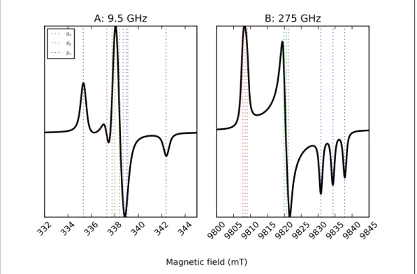
In real systems, it is often the case that both the hyperfine coupling and the g-factor are anisotropic. When the spectral resolution is not high enough, as in low-frequency EPR, it can

be arduous to discern the various contributions of the A andg tensors on the EPR spectrum.

At LF-EPR, such contributions might be hidden within the spectral linewidth, which is often

broader than the magnitude of the hyperfine coupling itself, for instance. This can be visualized

in Figure 1.5, where a spectral simulation is provided of a system such as a nitroxide radical

(like TEMPOL, see Chapters 3 and 4), which features an unpaired electron with spinS =1_/₂

interacting with a 14_{N nucleus with spin} _I _{= 1}_{. Both the} _g_{-factor and the hyperfine coupling}

are anisotropic, so that each of the three components of g is split into 2I + 1 = 3 lines, for

a total of in principle 9 lines. However, the 9.5 GHz spectrum of Figure 1.5 A shows a rather

(24)

1. INTRODUCTION

Figure 1.4: Energy diagram (not to scale) representing the effects of the spin Hamiltonian of Equation 1.12 for an electron spinS =1_/₂ _{interacting with a nuclear spin}_I _{= 1}_{. (A) When no}

external magnetic field is applied, the two spin statesms= +1/2andms=−1/2are degenerate. (B)

Upon application of a magnetic field, the electron Zeeman effect lifts the degeneracy of the electron

mS spin states. Here, the nuclear Zeeman effect is not taken into account yet, and the nuclearmI spin states are degenerate. When the g-factor is isotropic, a single transition arises (represented as a gray arrow), and a single-line EPR spectrum is observed (bottom). (C) A further splitting of the|mSmIispin states is caused by the nuclear Zeeman effect, which lifts the degeneracy of the nuclearmI spin states into 2I + 1 = 3 states. (D) As a result of the hyperfine coupling between the electron and the nuclear spin (here taken to be isotropic), the energy of the|mSmIispin states is shifted byaiso. Three transitions respecting the selection rules∆mS=±1and∆mI= 0arise (represented as red, green, and blue arrows), and the EPR spectrum will consist of 2I + 1 = 3 equally spaced lines (bottom).

splitting due to the Ax andAy components ofA are smaller than the spectral linewidth. The

red and green dotted lines indicate the field positions of, respectively, the transitions associated

to thegxcomponent and its Ax hyperfine component, and the transitions associated to thegy

(25)

to be discerned at 9.5 GHz, as shown by the peaks around 335 and 342 mT (the blue dotted line

represents the field positions of such transitions). All the other transitions are hidden within the

linewidth of the central peak around 339 mT, and cannot be resolved at the microwave frequency

of 9.5 GHz. However, going to HF-EPR offers a much clearer picture of the system under study.

In the spectrum of Figure 1.5 B, simulated for the microwave frequency of 275 GHz, the peaks

associated to the three transitions arising from the anisotropicg are clearly recognizable. The

hyperfine splitting of theAx andAy components is still too small as compared to the spectral

linewidth; however, theAzcomponent is large enough to give rise to three clearly separated lines

of thegz component around 9831, 9834, and 9837 mT. This example shows the advantages of

high-frequency EPR over low-frequency EPR also in determining the hyperfine components of a

paramagnetic system.

1.5.3 High-spin systems

So far, only the case of a single unpaired electron with spin S = 1_/₂ _{has been considered.}

However, it is fairly common to come across paramagnetic systems with spin higher than 1_/_2,

such as transition metal ions (like in Chapter 2), or several electron spins ferromagnetically

coupled (like in Chapter 5).

In a high-spin system such as a transition metal ion, the unpaired electrons of the d(or f)

orbitals are subject to a second-order effect of the spin-orbit coupling known as zero-field splitting

(ZFS), which is a term that adds to the system’s spin Hamiltonian and takes the following form:

HZF S =S·D·S (1.13)

where Drepresents the zero-field splitting tensor. The name originates from the fact that

such contribution does not depend on the external magnetic field, and an energy separation

between the spin levels is present even in the absence of an externally applied magnetic field,

being an intrinsic property of the system.

In Chapter 2 of this thesis, the paramagnetic system under study is ad5_{Fe(III) center, which}

turns from a high-spin (HS) S =5_/₂ _{state to a low-spin (LS)}_S ₌1_/₂_{state as a result of the}

replacement of its axial ligand, which induces a change in the strength of the crystal field. Figure

1.6 shows the zero-field splitting of the spin levels for HS-Fe(III). It can be noticed how, even

in the absence of an external magnetic field (B0 = 0), the spin levels (arranged in degenerate

(26)

1. INTRODUCTION

332 334 336 338 340 342 344

A: 9.5 GHz

gx

gy

gz

980

0

980

5

981

0

981

5

982

0

982

5

983

0

983

5

984

0

984

5 Magnetic field (mT)

B: 275 GHz

Figure 1.5: Simulated cw EPR spectra at 9.5 GHz (A) and 275 GHz (B) for an electron spin

S=1_/₂_{with anisotropic}_g_{-factor, with anisotropic hyperfine coupling with a}14_{N nucleus with spin}

I = 1. The colored dotted lines represent the field positions of the transitions associated to the

gx,gy, andgz components (in red, green, and blue respectively). Simulations are performed with EasySpin [31], with tensorsg= [2.0030,2.0058,2.0083]andA= [18,18,99]MHz set the same as for TEMPOL (see Chapters 3 and 4), and isotropic Voigtian linewidths (0.25 mT at 9.5 GHz and 0.5 mT at 275 GHz).

case, the zero-field splitting tensor is isotropic, and so large (D = 315 GHz [32]) that even at

room temperature only the lowest Kramers doublet (corresponding tomS±1/2) is populated,

and only transitions between themS = +1/2←→mS =−1/2levels can be observed.

Systems with spin higher than 1_/₂ _{can also be the result of separate electron spins at a}

distance such that they can interact with each other. The electron–electron interaction consists

of a classically-viewed dipolar contribution, and a quantum-mechanicalexchange contribution:

(27)

0 5 10 15 20 25 30 35 40 Magnetic field (T)

−4 −3 −2 −1 0 1 2 3 En er gy ( THz )

m

S = ±52

m

S = ±32

m

S = ±1 2

Figure 1.6: Simulated electron spin energy levels as a function of the external magnetic field for an

S=5_/₂_{system with isotropic}_g_{and isotropic}_D_{= 315 THz (from [32]). Simulations are performed}

with EasySpin [31] showing thexdirection.

where, in analogy to Equation 1.11, the first term is the electron Zeeman effect, the second

term is the dipolar coupling between the two electrons (D12being the dipolar coupling tensor),

and the third term is the exchange interaction between the two electrons (J12being the isotropic

exchange coupling). The subscripts refer to electron 1 or 2.

In Chapter 5 of this thesis, the paramagnetic intermediate of the enzyme under study is

suggested to be a triplet system composed of a Cu2+ ion interacting with a tyrosyl radical (an

organic radical), both with spin S =1_/_{2. Figure 1.7 shows the diagram of the magnetic field}

dependence of the spin levels of a simplified system, namely one where theg-factor is isotropic

and there is no hyperfine interaction with the spin of the copper nucleus. As a result of the

interaction of two spinsS=1_/_{2, an}_S _{= 0}_{and an}_S_{= 1}_{spin multiplicity are generated (named}

singlet and triplet, respectively), whose energy separation is proportional to the exchange coupling

J12. The mS = 1 state of the S = 1 spin multiplicity is further split from the mS = 0 and

mS =−1states by the dipolar coupling tensor D12 at zero field. Transitions are possible only

(28)

1. INTRODUCTION

0

20

40

60

80

100 Magnetic field (mT)

−10

−8

−6

−4

−2

0

2

4

6 En

erg

y (

GHz

)

S

= 1

S

= 0

m

S

=

+1

m

S

=

0

m

S

=

−1

Figure 1.7: Simulated electron spin energy levels as a function of the external magnetic field for a triplet system made of two interactingS=1_/₂_{electron spins, with isotropic}_g_{, isotropic exchange}

couplingJ12= 12 GHz, and anisotropicD12= [290,290,−580]MHz (from [30]). Simulations are

performed with EasySpin [31] showing thexdirection.

EPR transitions are called ”allowed” when they occur between spin levels with selection rule

∆mS = ±1. However, at LF-EPR, weaker transitions arise, called ”forbidden”, that deviate

from the aforementioned selection rule and, in the case of a triplet state, occur between spin

levels with ∆mS = ±2. These transitions, also called half-field transitions, occur when the

Zeeman terms of the spin Hamiltonians of Equations 1.13 and 1.14 (which are field-dependent)

are small in comparison to the ZFS or spin-spin interaction terms – in other words, when the

external magnetic field is low or, equivalently, when the EPR microwave frequency is low. Under

such circumstances, the spin levels are not well-defined by single magnetic quantum numbers,

but rather are a mix of them. The abundance of half-field transitions at LF-EPR makes the

resulting spectra extremely hard if not impossible to interpret, especially with systems with spin

S > 1. However, the spin levels of such systems are ”well-behaved” at high magnetic field,

namely when the Zeeman terms are bigger than the ZFS or spin-spin interaction terms, meaning

that the single spin levels can be correctly described by their magnetic quantum numbers, and

(29)

and interpretation of high-spin systems.

1.5.4 Slow-to-fast motion and rigid limit in EPR spectra

All the EPR spectra shown thus far originate from samples in the so-calledrigid limit, namely

samples whose paramagnetic species are not free to quickly rotate in any direction – a situation

proper of solids. When this is the case, the paramagnetic species in a solid matrix are bound

to a specific direction, and so are their electron spins. Such a rigid system is susceptible to

the orientation of the external magnetic field as compared to the orientations of its own

spin-Hamiltonian parameters, and the anisotropy (when present) is observable in the EPR spectra.

In particular, powders and frozen solutions (i.e., disordered glasses) can be seen as ensembles

of spins ranging all possible spatial directions – as opposed to single crystals, which have all

of their spins oriented in the same direction, thus giving rise to EPR spectra associated to one

specific spatial orientation. When the EPR spectrum of a powder is recorded (hence also called

powder spectrum), the spin transitions of all possible orientations are induced, and a continuous absorption is measured. In practice, however, the resulting powder spectrum does not look like

a continuous absorption as a result of the field modulation employed to record the spectrum,

which causes it to appear like a first-derivative spectrum. All the spectral simulations shown

before correspond to powder spectra.

The complete opposite case as that of a powder spectrum is when the paramagnetic species

are freely rotating in their medium, a situation that normally occurs with molecules in solutions,

and that is referred to asfast motion. Due to the fast rotational motion (or ”tumbling”) of the

paramagnetic species in the solution, all the anisotropic terms of the system’s spin Hamiltonian

average out. What is thus visible in the EPR spectrum of a paramagnetic species in a solution

is the mean value of thegtensor and the isotropic component (aiso) of the hyperfineAtensor.

The components of the D tensor average to zero in the fast-motion regime and the zero-field

splitting is thus not measurable.

An intermediate situation between the rigid-limit and the fast-motion regimes also exists,

namely when the medium containing the electron spins still allows rotational motion of the

paramagnetic species, but such motion is hindered by physical factors such as the high viscosity

of the solution (which is the case for the mixtures of water and glycerol described in Chapters 3

and 4) or steric effects (such as a spin label attached to a protein). As a result of these hindrance

effects, the rotational motion of the paramagnetic species is slowed down or, equivalently, their

rotational correlation time (τc) becomes longer, which affects the spin relaxation processes and

(30)

1. INTRODUCTION

rotates by one radian in a certain spatial direction, and it ranges from picoseconds for the

fast-motional regime, to nanoseconds up to microseconds for the slow-fast-motional regime. There are

several models to describe such slow-motion effects (like the Stokes-Einstein equation used in the

Appendix to Chapter 3 of this thesis), through which valuable information on the surroundings

of a spin system can be obtained, such as the temperature of a solution, or the conformation of

a spin-labeled protein.

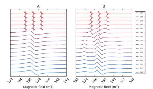
Nitroxide radicals such as TEMPOL exhibit important changes of the spectral line shape as a

function of their rotational correlation time. This is shown, as an example, in Figure 1.8, where

the spectral linewidth changes of solutions of TEMPOL are plotted as a function of the sample

temperature (in the range between 143 K and 293 K). A different dependence of the solution’s

viscosity on temperature affects the spectral shapes differently, so that a solution of TEMPOL

in pure water (A), and a solution of TEMPOL in a mixture of water and glycerol 1:1 in volume

(B) behave very differently as a function of temperature. Since the viscosity of liquid water does

not change much with temperature, the mobility of the molecules in the solution is fast and

roughly constant. This can be seen in the spectra of Figure 1.8 A in the temperature range

from 293 K down to 253 K, where the spectral line shape does not change much. The

three-line spectrum originates from the aiso component of the hyperfine interaction of the electron

with the 14_{N nucleus, as the anisotropic component is averaged to zero as a result of the fast}

rotational motion of the molecules in the solution. From 243 K down, the solution freezes and

a powder spectrum arises, which has however an unusual shape. This is due to the fact the

TEMPOL molecules, at a relatively high concentration, form clusters in the absence of glycerol

in solution, becoming close enough to each other for their spins to interact intermolecularly,

which results in a broadening of the line shape. Figure 1.8 B shows a rather different situation,

because the viscosity of water and glycerol solutions varies greatly with temperature, affecting

the rotational motion of the molecules and thus the spectral shape. A progressive spectral

broadening is visible in the temperature range between 263 and 233 K, this being the range

where the sample transitions from a fast-motion regime through a slow-motion regime, down to

a rigid-limit regime. The plot of Figure 1.8 B highlights the importance of glycerol added to the

solution, which has a ”de-clustering” effect on the TEMPOL molecules. As a result, the changes

in the spectral line shape of TEMPOL are easy to interpret and simulate, yielding information

(31)

332 334 336 338 340 342 344

Magnetic field (mT)

A

332 334 336 338 340 342 344

Magnetic field (mT)

B

293 K 283 K 273 K 263 K 253 K 243 K 233 K 223 K 213 K 203 K 193 K 183 K 173 K 163 K 153 K 143 K

Figure 1.8: 9.5 GHz cw EPR spectra of solutions of TEMPOL at a concentration of 2 mM, (A) in pure water and (B) in a mixture of water and glycerol 1:1 in volume. The spectra were recorded with a Bruker Biospin EMX 080 EPR spectrometer, in the temperature range between 143 K and 293 K, controlled by a nitrogen-flow cryostat ER4131VT temperature control system (Bruker).

1.5.5 Home-built 275 GHz EPR spectrometer

The EPR spectra at the microwave frequency of 275 GHz described in this thesis were performed

on a spectrometer built around 2000 by Blok and coworkers at Leiden University, and described

in great detail by the same authors in [34]. The construction of such spectrometer was driven

by ever-growing interest in HF-EPR, after spectrometers at frequencies such as 95 and 140 GHz

became commercially available.

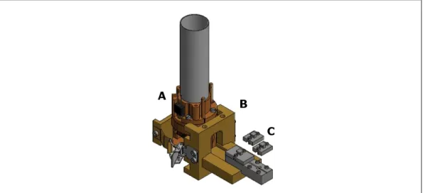
Here, a brief description of the setup is provided. A simplified block diagram of the home-built

275 GHz EPR spectrometer is shown in Figure 1.9, and consists of four main parts:

(A) Two microwave sources, producing two microwave beams at the frequencies of 91.9 GHz

and of 89.7 GHz, which are sent to diode triplers that return the frequencies of 275.7 GHz

and 269.1 GHz. The former is the frequency used to excite the sample, while the latter

(32)

1. INTRODUCTION

(B) A microwave bridge operating in reflection mode, suitable for both cw and pulsed

experi-ments. It transmits the incoming microwave frequencies to and from the resonant cavity

with a quasi-optical transmission setup, which allows the confined beams of

electromag-netic waves to travel in free space, thus making the transmission losses negligible – as

opposed to conventional waveguide technologies at such high frequencies.

(C) A single-mode, tunable resonant cavity which is located at the bottom of a

variable-temperature helium-gas flow cryostat placed at the center of a superconducting magnet.

The cavity is coupled to the microwave bridge through a corrugated circular waveguide

whose geometry maximizes the microwave coupling and minimizes the transmission losses.

The cavity has an absolute sensitivity as high as 108_{spins per mT. The cylindrical cavity}

has a diameter of 1.4 mm and a length between 0.8 and 1.4 mm that can be varied with

two plungers located at both sides, which move synchronously and symmetrically inward

and outward so as to allow the tuning of the cavity. Underneath the cavity is a coil that

generates the field modulation for cw experiments, and a grid that allows irradiation of

the sample from an external source.

(D) A superconducting solenoid magnet capable to reaching 14 T. The scan-to-scan field

stability is less than 0.1 mT, while the day-to-day field stability is less than 1 mT.

The microwave beam reflected from the resonant cavity, carrying the EPR signal, is

trans-mitted through the corrugated waveguide back to the bridge, where it reaches a Martin-Puplett

diplexer, which combines the EPR signal at 275.7 GHz with the local oscillator at 269.1 GHz,

giving both the same well-defined polarization. The coupled output signal is then directed to

a polarization-sensitive microwave mixer where a signal is produced at the so-called

intermedi-ate frequency (IF) of 275.7−269.1=6.6 GHz. The IF signal is finally amplified and fed to a

(33)

(34)

(35)

(36)

2

Effective coupling of Rapid

Freeze-Quench to High-Frequency

(37)

2.1 Introduction

Determination of reaction rates and detection of short-lived intermediates of fast chemical

reac-tions are an important goal in those fields that involve molecular chemistry, such as biochemistry,

pharmaceutics, medicine, environmental science, and material science, to name a few.

Kinet-ics and intermediates shed light on the mechanism of a reaction, which in turn yields broader

information about the chemical system under study.

One possible stratagem to investigate chemical kinetics is that of letting the reaction unfold

for controlled time steps and then ”freezing” it. In this way it is possible to follow the decay

and growth of reactants and products, or the evolution of reaction intermediates. One of the

most widely used techniques to attain this is called Rapid Freeze-Quench(RFQ), in use since 1961 [18], which is often coupled to Electron Paramagnetic Resonance (EPR) in view of the

paramagnetic nature of the intermediates of a great deal of chemical reactions.

The multi-frequency approach in EPR is of particular interest, namely when low-frequency

experiments (e.g. those at the standard frequency of 9.5 GHz, called X-band) are combined

with high-frequency ones (HF-EPR, e.g. those at microwave frequencies of 95 and 275 GHz).

Such approach offers a better and more complete characterization of the magnetic system under

study. However, collection of RFQ samples is – to say the least – problematic for applications in

HF-EPR, because the size of HF resonant cavities is hugely reduced as compared to the standard

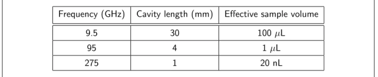
9.5 GHz EPR, thus making the sample holders and the sample volume dramatically small. In

Table 2.1 is shown a comparison of the typical sample volumes used for three EPR frequencies,

namely 9.5, 95, and 275 GHz. The sample volume downsizes by about 104_{times going from low}

to high frequency. It is therefore vital to develop a sample packing technique that guarantees

an efficient, homogeneous, and reproducible sample collection in the small capillaries used as

sample holders for HF-EPR.

Frequency (GHz) Cavity length (mm) Effective sample volume

9.5 30 100 µL

95 4 1µL

275 1 20 nL

(38)

2. EFFECTIVE COUPLING OF RFQ TO HIGH-FREQUENCY EPR

In the literature there have been endeavors to implement and standardize packing techniques

for RFQ-EPR applications [35] [36] [37] [38] [39] [40] [21].

Ballouet al.[35] and Oellerichet al.[36] are the earliest reported attempts to study a chemical reaction detected with X-band EPR on a timescale of less than 80 ms. Although of great interest

given the short timescale, both authors attribute the large inaccuracy on the reaction rates (errors

bigger than 10%) to the nonuniform and irreproducible packing of the RFQ particles. Indeed,

in both papers the authors report a rather low and nonhomogeneous packing efficiency, between

0.5 ÷ 0.7 the former, and between 0.4 ÷ 0.6 the latter. Oellerich even concludes that this

problem constitutes an ”intrinsic deficiency of freeze-quench EPR spectroscopy”, and indeed, as

described below, this is a serious issue not easily circumvented.

Namiet al.[37] propose an improved method to collect and pack RFQ particles from an

isopen-tane suspension, based on pumping said suspension through an EPR tube in which a filter has

been placed. The RFQ particles are trapped at the filter and the isopentane is easily removed.

The advantages of this method are its reproducibility and efficiency: the authors report a

pack-ing factor between 0.68÷0.76, which is indeed a considerable improvement, also compared to

previous studies (see below). A slightly modified version of this method is applied in this work.

Schuenemann et al.[38] are the first to report the application of RFQ to HF-EPR in a multi-frequency EPR study (at 9.6, 94, 190, and 285 GHz), on a timescale of up to 40 ms. Although

HF-EPR implies dealing with sample holders of reduced size, the method used by the authors

to pack the RFQ for HF-EPR is basically the same as for low frequency, i.e., compacting the

sample sprayed in a tube of the appropriate size by means of a metal rod. However, the authors’

focus is to detect the reaction intermediate of the reaction under study, rather than its reaction

rate, so that inhomogeneous sample packing is of no concern to them.

In the context of RFQ-HFEPR, Manzerova et al. [39] bring about an innovative method to

freeze-quench reactants, reduce them to fine particles, and collect them. They report a

technol-ogy based on rotating copper wheels kept at a temperature of 80 K, on which the mixture of the

reactants is sprayed through a home-built nozzle. The reactant mixture is thus freeze-quenched,

and the sample is then ”scraped” off the wheels and collected by tapping with a capillary suitable

for 130 GHz EPR. Although such approach introduces the advantage of not having to handle

static frozen particles floating in isopentane, the packing factor the authors report is 0.5, thus

being no improvement as compared to those from the aforementioned studies.

All of the aforesaid publications require a large amount of sample, which is often a disadvantage

when working with biological samples. Kaufmannet al. [40] and Pievo et al.[21] reported the development of, respectively, a micro-fluidic mixer (after its introduction by Cherepanov and de

(39)

for RFQ-HFEPR studies of biological samples. It is interesting that Kaufmann also implemented

a new way of collecting the RFQ samples, based on the idea of Manzerova [39]: they use a

rotating aluminum plate kept at a temperature of 80 K, on which the reagent mixture is sprayed

and freeze-quenched. The RFQ powder is then collected by tapping the capillary on it. However,

the packing efficiency is not mentioned, while in [21] a packing factor of 0.5÷0.6 is reported.

From the cited literature thus emerges a serious difficulty in RFQ-HFEPR when it comes to

collect RFQ particles and study them in a standardized, efficient, and reproducible way.

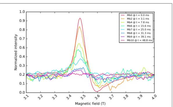
In the literature, a common and practical way of testing the performance of RFQ-HFEPR is

making use of the binding reaction of sodium azide to myoglobin. This reaction (Scheme 2.1)

is a well-understood model system that offers several advantages in EPR studies because of its

convenient spectral properties [35] [36] [21].

[Fe3+_HS—OH2] +N−3 →[Fe 3+

LS—N

−

3] +H2O (2.1)

Myoglobin (abbreviated Mb) is an iron- and oxygen-binding hemoprotein, similar to hemoglobin,

whose function is that of reversibly storing and transporting oxygen in the muscle tissues of many

vertebrates [41]. At neutral pH, the heme iron (Fe(III), ad5ion) of ferric myoglobin (also known

as met-myoglobin) exhibits an octahedral coordination environment with one of the axial po-sitions being occupied by variable ligands. The nature of such variable ligands determines the

energy splitting between the upper and lower groups ofd orbitals. Water can be one of these

ligands, and weakly binding to the heme-Fe(III), thus generating a high-spin (HS)S=5_/₂_state.

However, when an exogenous strong-binding ligand such as azide (N−₃) replaces the axial water

molecule, the stronger ligand-field effect induced on Fe(III) converts its spin state to low-spin

(LS) withS=1_/_{2. Scheme 2.1 illustrates the binding reaction of azide to myoglobin.}

The spectral features of HS- and LS-Fe(III) are completely different, the former having an

in-tense signal aroundg= 6, while the latter having a rhombic signal aroundg= 2. Such features

turn out to be so handy that the binding reaction of sodium azide to myoglobin has become a

standard when evaluating RFQ-EPR methods, both at low and high frequency [35] [36] [39] [21].

The present work originates from the premises cast by Nami in her PhD thesis [42], who

explored the feasibility of multi-frequency EPR coupled with RFQ making use of the binding

reaction of sodium azide to met-myoglobin, based on an improved method to pack and load

cap-illaries for HF-EPR [37]. However, her investigations at high-frequency EPR (95 and 275 GHz)

yielded unconvincing results, given the huge scatter of the data points. The two main limitations

(40)

• The reaction time scale selected for the study was very short, namely less than 10 ms for a reaction with a characteristic time twice as long;

• The manganese(II) ions introduced in the RFQ samples, used for internal calibration, were originally mixed in the sodium azide solution, rather than in the myoglobin solution. In this

way, theMb_/_Mn2+_{ratio is affected by possible irreproducible mixing of the RFQ apparatus,}

which results in an inconstant ratio for different RFQ samples.

For these two reasons, in this work it was chosen to select a longer time scale for the myoglobin

reaction of Scheme 2.1 (namely, up to∼50 ms), and to add MnCl2 to the myoglobin solution,

rather than to the sodium azide solution, prior to mixing in the RFQ apparatus.

Another critical aspect of this study is the packing of the RFQ samples in the sample holders

suitable for 275 GHz EPR, namely quartz capillaries with an inner diameter of 150µm, hosting

a sample volume of 20 nL in the resonant cavity. While the general procedure to prepare the

X-band RFQ samples is the same as described in [42], an improved method for sample preparation

for 275 GHz was devised.

2.2 Experimental

2.2.1 Materials

Equine-heart met-myoglobin, sodium azide (NaN3), and DMSO were purchased from

Sigma-Aldrich (cat. n. M1882-1G, 15,795-3, and 154938-1L respectively). MnCl2 was purchased from

Baker Chemicals (cat. n. 0173). Myoglobin was dissolved in phosphate buffer 100 mM at

pH 7.8, with the addition of 5% v/v DMSO and 50 µM of MnCl2, to form a solution with

concentration 2.4 mM. Sodium azide was dissolved in phosphate buffer 100 mM at pH 7.8 to

form a solution with concentration 24 mM. After RFQ mixing, the Mb:azide ratio is 1.2:12 mM.

The concentration of the myoglobin solution was determined spectrophotometrically using the

extinction coefficient505=9.7 mM−1 cm−1.

2.2.2 Sample preparation

Ten RFQ samples (named Mb1 to Mb10) were prepared with the same RFQ apparatus and

method described in [37] (2-mL syringes, ram velocity 3.2 cm s−1, displacement 3 mm), at a

(41)

ten samples were initially measured at 9.5 GHz, and later (about a year after), the same were

used for measurements at 275 GHz.

Table 2.2 summarizes, for each RFQ sample, the corresponding reaction time, that is calculated

from the parameters used in the RFQ setup, and not corrected by the so-calledfreezing time.

RFQ sample label Mb1 Mb2 Mb3 Mb4 Mb5 Mb6 Mb7 Mb8 Mb9 Mb10

Calculated reaction time (ms) 2.0 3.1 4.9 7.8 9.8 15.6 25.0 31.3 39.1 48.8

Table 2.2: Calculated reaction time of the RFQ samples.

In addition, two myoglobin solutions without any sodium azide were prepared (labeled Mb0),

meant to represent reaction 2.1 before it has started, namely at t = 0. For the spectra at

9.5 GHz, the Mb0 solution was prepared from the same batch used to prepare the RFQ samples.

However, for the spectra at 275 GHz, since about a year passed from the preparation of the RFQ

samples, the Mb0 solution was made from an independent batch, but with identical composition

as described in Subsection 2.2.1.

Sample packing for 9.5 GHz EPR

The preparation of RFQ samples for 9.5 GHz EPR is a procedure that was successfully

standard-ized by Nami [37]. With this procedure, the RFQ samples are straightforwardly packed in quartz

tubes, readily used as sample holders for 9.5 GHz EPR. The essential steps of this procedure,

conducted in a polystyrene box filled with dry ice pellets, are briefly reported below:

• The quartz tubes (10 cm long, 3 mm inner diameter) are open on both sides, and are cus-tomized by tapering them on one side. This allows the accommodation of a polypropylene

disk used as a filter.

• The tapered end is connected through a latex tubing to a hand-held 60-mL Norm-Jet disposable syringe used to create underpressure (instead of a water aspirator, as described

in the original procedure).

• While manually creating underpressure in the syringe, the other side of the quartz tube is dipped in cold isopentane contained in a vial in contact with dry ice. The isopentane is

(42)

• By maintaining the underpressure in the syringe, the pre-cooled quartz tube is quickly transferred into the vial containing the RFQ sample in cold isopentane. This vial has

previously been lain on dry ice to ensure thermal contact. By pushing the quartz tube

to the end of the sample vial (and making sure that the filter-containing tapered part is

always in contact with dry ice so as to prevent the sample from warming), the RFQ sample

is sucked up the tube and accumulates through it thanks to the filter. With the settings

of the RFQ apparatus described above, a 3-mm quartz tube is typically filled with roughly

4 to 5 cm of sample.

• When all the isopentane contained in the sample vial has been aspirated, the latex tubing is cut and the quartz tube is stored in liquid nitrogen. As opposed to the procedure described

in [42], the sample in the tube is not further packed more tightly with a steel rod because

of the relatively big amount of sample present in the tube, and because a tighter packing

would result in a more difficult handling for applications at 275 GHz (see 2.2.2).

The quartz tubes prepared in this way are ready to be measured with a 9.5 GHz EPR

spectrometer, and do not need further treatments.

Sample packing for 275 GHz EPR

The preparation of RFQ samples for 275 GHz EPR is by far more complicated than for 9.5 GHz

EPR. The minuscule size of the capillaries used as sample holders (150µm inner diameter) poses

a twofold problem. Firstly, accidental warming of the samples is easy and fast, in view of the

tiny volumes involved. For this reason, since the warming of the samples has to be avoided at

all costs, they have to be handled at cryogenic temperatures. This leads to the second issue,

which is the difficulty of handling such small capillaries in a cryogenic atmosphere, while wearing

cryoprotective gloves that reduce the user’s hand sensibility.

A successful sample packing in capillaries for 275 GHz EPR is thus a troublesome procedure

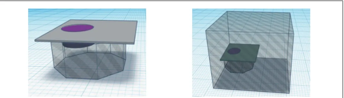
that requires a trained operator. Following is a description of the basic steps of this procedure

(as reported in essence in [42]), which is carried out in a polystyrene box half-filled with liquid

nitrogen. Thanks to a flow of cold nitrogen gas blowing on the surface of the liquid nitrogen,

the average temperature in the box within the first 10 cm from the liquid nitrogen surface is

kept below -100°C.

• A home-built stainless-steel plate (15×15 cm) is placed on top of an octagonal polystyrene box (14 ×14×6 cm). The plate has a central hole (6 cm diameter) that accommodates

an agate mortar (whose surface sits at the same height as the plate), tightened with

T-CYCLE EPR Development at 275 GHz for the study of reaction kinetics & intermediates

The handle

http://hdl.handle.net/1887/68233

ho

lds various files of this Leiden University

dissertation.

Author: Panarelli, E.G.

Title:

T-CYCLE EPR Development at 275 GHz for the study of reaction kinetics &

intermediates

T-CYCLE EPR

Development at 275 GHz for the study

of reaction kinetics & intermediates.

Proefschrift

Enzo Gabriele Panarelli

Contents

1

1.1

Motivation and scope

1.2

Chemical kinetics

Time

Co

nc

en

tra

tio

n

A

I

P

1.3

Rapid Freeze-Quench

1.4

Laser-induced Temperature-jumps

1.5

Electron Paramagnetic Resonance

1.5.1

The electron Zeeman effect and the

g

-factor

0 50 100 150 200 250 300 350 400

Magnetic field (mT)

−8

−6

−4

−2

0

2

4

6

8

En

e g

y (

GHz

)

A: 9.5 GHz

800

0

850

0

900

0

950

0

100

00

105

00

Magnetic field (mT)

−200

−150

−100

−50

0

50

100

150

200

₁₀₀

₁₀₅