Prepared for submission to JCAP
Testing Predictions of the Quantum
Landscape Multiverse 2: The
Exponential Inflationary Potential
Eleonora Di Valentino
1,2Laura Mersini-Houghton
31Institut d’ Astrophysique de Paris (UMR7095: CNRS & UPMC-Sorbonne Universities),
F-75014, Paris, France
2Sorbonne Universités, Institut Lagrange de Paris (ILP), F-75014, Paris, France
3Department of Physics and Astronomy, UNC-Chapel Hill, NC 27599, USA
Abstract. The 2015 Planck data release tightened the region of the allowed inflationary
models. Inflationary models with convex potentials have now been ruled out since they
produce a large tensor to scalar ratio. Meanwhile the same data offers interesting hints on possible deviations from the standard picture of CMB perturbations. Here we revisit the predictions of the theory of the origin of the universe from the landscape multiverse for the case of exponential inflation, for two reasons: firstly to check the status of the anomalies associated with this theory, in the light of the recent Planck data; secondly, to search for a counterexample whereby new physics modifications may bring convex inflationary potentials, thought to have been ruled out, back into the region of potentials allowed by data. Using the exponential inflation as an example of convex potentials, we find that the answer to both tests is positive: modifications to the perturbation spectrum and to the Newtonian potential of the universe originating from the quantum entanglement, bring the exponential potential, back within the allowed region of current data; and, the series of anomalies previously predicted in this theory, is still in good agreement with current data. Hence our finding for this convex potential comes at the price of allowing for additional thermal relic particles, equivalently dark radiation, in the early universe.
Contents
1 Introduction 1
2 Convex Potentials 2
2.1 Exponential Potential 3
3 Method 5
4 Results: Modified Exponential Inflation 7
5 Conclusions 11
1 Introduction
How were the initial conditions of the universe selected? Probing this fundamental questions is key to understanding the universe we inhabit. Fortunately, major advances in precision
cosmology, notably the Planck data [5,6] and SN1a data [8] recently, place us in an unusually
favorable position - for the first time we can test and falsify theories that extend physics beyond inflation and the standard model of cosmology.
In previous work [1–4], we developed a theory of the initial conditions of the universe
from a quantum multiverse. The selection of the initial states was derived from the quantum dynamics of gravity acting on the string landscape, which we took as our working example for the configuration space of initial states. Allowing the wavefunctional of the universe to propagate through the landscape vacua, enabled us to derive the most probable wavefunction
solution by means of the quantum cosmology formalism. The wavefunction operated on
a minisuperspace spanned by the scale factor a of 3-geometries and the landscape moduli
variables φ with the landscape vacua energy profile, the potential V(φ). The solutions we
found, with the decoherence among branches included [2] showed why high energy inflationary
states are natural.
Tracing out long wavelength modes of metric and matter fluctuations decohered the
wavefunction of the universe [2,3]. Since coherence and decoherence are closely related, the
latter induced a nonlocal entanglement among all surviving branches of the wavefunction, localized at various high energy landscape vacua, and which give rise to universes like ours. We calculated the strength of the entanglement of our branch with others for convex potentials
in [3], and for concave potentials in [4], and the modifications it induced on the Friedmann
equation and the gravitational potential of the universe. The energy of landscape vacua varies
across the landscape. This energy for each vacuum is denoted by the parameter b, which is
local since it differs from one vacuum to the next. Assuming that locally the vacuum states
may acquire their energy from SUSY breaking, we herein refer to the parameter b as the
’SUSY breaking parameter’. It is possible that vacua may acquire their energy b from some
other mechanisms instead of SUSY breaking. Therefore, b should be seen as a label of the
individual vacuum energies independently of the mechanism that produced them.
In this work we analyze the status with the predictions of this theory of the origin of
the universe from a quantum landscape multiverse [1–4], against the most recent Planck data
inflationary potentials was given in [7]. The modifications to the perturbation spectrum and the Newtonian potential of the universe, originating from quantum entanglement in this
theory, were derived in [3] for the case of exponential inflation. We review the main results
below. In its simplest and unmodified form, based on a 6 parameter model of standard cosmology, the exponential inflationary potential is already ruled out. In fact based on the 6 parameter model of the standard cosmology, Planck’s recent bounds on the tensor to scalar
ratio r rule out most of the convex potentials, since they predict larger’s.
The aim of our study here is two fold: firstly we aim to compare the predictions of the theory of the origin of the universe from the quantum multiverse against the recent measurements made by Planck for convex potential such as the exponential model; secondly, we wish to demonstrate that if the standard model of cosmology were extended to allow for new physics then convex inflationary potentials that in the simple picture were thought to be ruled out by data, may not in fact be ruled out in the extended picture. The analysis
of concave downard potentials, specifically the Starobinsky model, was done in [7]. The
point of choosing the exponential inflation as the object of our study of convex potentials, is not to advocate that this is how our universe started. Rather, we hope that by providing a counterexample to the standard interpretation of observations, in our case the chosen example is the exponential potential, may help to emphasize a key point, namely: data and our understanding of observational results are two different things. That is, ruling out models of inflation is not straightforward if we allow the 6 parameter standard model of cosmology to be extended to new physics realms.
The paper is organized as follows: in Section 2 we first review the main results of the
modified spectra, field solutions and Friedmann equation for the exponential potential of
[3], in the context of the theory of the origin of the universe from the quantum landascape,
since we need these expressions for the data analysis. In Section 3 we present the method
of analyzing the predictions of this theory against data, provide the results in Section 4, and
conclude in Section 5.
2 Convex Potentials
In contrast to concave downward inflationary potentials, studied in [4, 7] for the case of
Starobinsky potential, the exponential inflationary model is a convex potential with V00 >0
. In convex inflationary models like the exponential model, the mass term which drives
fluctuations is V00 = m2 > 0. Fluctuations are small and stable in these potentials when
expanded around the minimum. The correction to the Friedmann equation derived in [3]
for convex potentials, is: Vef f == V − 12 V
2
9M4F[b, V] = V +
1 2
V2
9M4|F[b, V]| in Eq. 2.1, since
F[b, V]<0and m2 =V”>0.
Einstein equations are modified accordingly since the inflaton potentialV is now replaced
by the modified inflationary potential Vef f, which besides its dependence on the field φ,
also depends on the landscape ’Susy breaking parameter’ b . Vef f encaptures the nonlocal
entanglement between our wavefunction branch and other branches. The energy correction term in Vef f
Vef f =V −f[b, V] =V +|f[b, V]| (2.1)
f(φ) = 1 2
V(φ) 3M2
P 2
F(φ) (2.2)
with b the landscape parameter describing the energy scale from ’SUSY breaking’ in
each vacua. The entanglement information contained in F[b, V] was derived in [3], and is
given by
F(φ) = 3 2
2 +m
2M2 P
V(φ)
Log
b2MP2 V(φ)
−1 2
1 +m
2
b2
e−
3b2MP2
V(φ) (2.3)
The Friedman equation of expansion becomes
3Mp2H2 =Vef f =V −f[b, V] (2.4)
for convex potentials. We apply these modifications to the exponential potential as an example of applying the quantum entanglement modifications in the theory of the origin of the universe from a quantum landscape to the convex types. The field solution is
modi-fied accordingly since the inflationary potentialV(φ) is replaced with the modified potential
Vef f(φ, b). The field solution is obtained from the field equation
3Hdφ/dt=−∂Vef f
∂dφ (2.5)
Using dφ/dt=Hdφ/dlnk,the field equation Eq. 2.5, from Eq.2.4, becomes
dN = Vef f
M2 pVef f0
dφ=−dlnk (2.6)
We assume the correction term is small compared to the leading term V i.e. slow
roll holds even with correction terms. Then we can approximate the integral in Eq.2.6 as:
R Vef f
V0
ef f
dφ'11−−df /dVf /V R V V0.
This last equation 2.6 gives us the field as a function of k, or equivalently the number
of efoldsdN. IntegratingdN from the start to the end of slow roll, allows us to get the total
number of efolds N.
2.1 Exponential Potential
Let us now apply these modifications to the exponential potential as an example of the mod-ified convex potentials reviewed above. The derivation of modifications to the perturbation spectrum and the Newtonian potential of the universe, and the series of predictions resulting
from these modifications were derived in [3]. However the only data available then was the
first release of WMAP data. One of our goals here is to check the status of the predictions
made in [3], and specifically the status of anomalies we predicted there over a decade ago, in
the light of the most recent Planck data release [5,6] and the new release of the SN1a data
of Riess et al. [8].
The pure unmodified exponential potential, introduced the first time by [9], is
V(φ) =V0e
−λφ
MP (2.7)
V0(φ) =−V0λ
MP
e− λφ
MP (2.8)
The curvature of the potential is positive and the mass squared term which drives the
fluctuations, is given by the curvature V00 evaluated at the start of slow roll. So far, the
expression for the effective potential and the correction termf(b, V)are provided with respect
to Mp which denotes the normal Planck mass.
The mass term that drives the fluctuations is
m2=V00(φin) =V0
λ MP
2
e−λφinMP ≈ V0λ
2
M2 (2.9)
The quantities we need for carrying out the data analysis in the next section, such as
the power spectrum, field solution, the tensor and scalar index, are calculated [3] from the
modified potential which includes the correction term Vef f. The derivative of the effective
potential is
Vef f0 (φ) =V0(φ)(1−df(φ)/dV) (2.10)
where
df
dV =
V
9M4 p
F[b, V] +V
2dF/dV
(2.11)
and
dF
dV =−
3
m2Mp2−M2(b2+m2)Exp[−3b2Mp2
V ]−2V −m2Mp2Log[
b2M2
p
V ]
2V2 (2.12)
The second derivative of the effective potential needed below is
Vef f00 (φ) =V00(φ)
1− df
dV
− d
2f
dV2V
02 (2.13)
where V00 = (λ/Mp)2V. The unmodified field solution for the exponential potential
obtained from integrating the field equation, gives
φ0(k) =λMPln
k k∗
(2.14)
In the presence of modifications, with the potentialVef f, the field satisfies the equation
Vef f
M2 pVef f0
dφ=−dLn(k) (2.15)
which is integrated to give the modified field solution
φ(k) =λMPln
k k∗
"V0 ef f(φ0)
V0(φ
0) #
V(φ0)
Vef f(φ0)
=φ0(k)
(1−df /dV)
(1−f /V) (2.16)
We assumed that slow roll holds in the presence of modification, i.e the condition
∆Vef f
less than 7orders of magnitude during the slow roll regime, which allows us to pull them out of the field integral and approximate f(b, V)andf0(b, V)with their value at the start of slow roll.
We can now put everything together to calculate the power spectrum and tensor to scalar ratio. Note that the expressions of the spectra are defined with respect to the reduced
Planck mass, obtained from the Planck mass by a rescaling of Mp with: Mp/
√
8π). Since in what follows our data analysis and spectra are estimated with respect to the reduced Planck
mass, then we can continue using the reduced Planck mass and equivalently rescale b by the
factor of √8π becausebalways enters in a ratiob/Mp in the above modifications.
Pζ(k) =
1 24π2M6
P "
Vef f(φ)3
Vef f0 (φ)2 #
' 1
24π2M6 P
V(φ)3
V0(φ)2
(1−f /V)3
(1−df /dV)2 (2.17)
All unmodified quantities are denoted by0, egφ0, r0, P0 etc, mean unmodified and they
are evaluated with respect to the unmodified fieldφ0[k]. All modified quantites are evaluated
with respect to the modified field solutionφ[k]. The modifed tensor to scalar ratio is
r[k] = 8Mp2 V 0
ef f(φ)
Vef f(φ) !2
(2.18)
To calculate P[k], r[k], n[k]we only need V0 andVef f0 which we calculated above. With the above reminder that the modified field solution must be used to estimate the modified quantities, we can approximately relate r[k] to r0[k] by r[k]≈ r0[k]((1(1−−df /dVf /V)))2, bearing in
mind that in the approximate relation of r[k] with r0[k]both are evaluated with respect to
φ, not φ0.
From the modified power spectrum we can then calculate the modified scalar index
n[k]−1 = dLog(P[k])/dLog(k) with P[k] given above. The unmodified scalar tensor is
n0[k]−1 = dLog(P0[k])/dLog(k) where the 0 notation means unmodified field and power
spectrum and scalar tensor.
3 Method
We explore the modified Exponential model, by considering the 8 cosmological parameters
listed in the following, that are explored within the range of the conservative flat priors
reported in Table 1. We vary the 4 standard parameters of theΛCDM, namely: the baryon
Ωbh2 and the cold dark matter energy densities Ωch2, the reionization optical depth τ and
the ratio between the sound horizon and the angular diameter distance at decoupling Θs.
Moreover, we consider3inflationary parameters: the effective inflationary potential parameter
λ (see eq. 2.7), the energy scale of the inflation 1010V0/M4, and the contribution of the
primordial gravitational waves with a tensor-to-scalar ratio of amplitude r at the pivot scale
k0 = 0.002hM pc−1. Finally, we have the natural logarithm log(
√
8πb[GeV]) of the
SUSY-breaking scale associated with the landscape effectsb. As a second step, we consider extensions
to these baseline model, by adding the effective number of relativistic degrees of freedomNeff.
In Fig. 1 we show the temperature and polarization CMB angular power spectra by
varying the SUSY-breaking scale bassociated with the landscape effects.
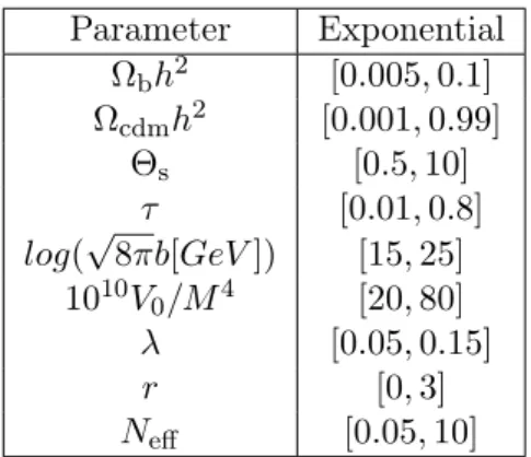
Parameter Exponential
Ωbh2 [0.005,0.1]
Ωcdmh2 [0.001,0.99]
Θs [0.5,10]
τ [0.01,0.8]
log(√8πb[GeV]) [15,25] 1010V0/M4 [20,80]
λ [0.05,0.15]
r [0,3]
Neff [0.05,10]
Table 1. External priors on the cosmological parameters assumed in this work.
100 101 102 103 104
` 0 1000 2000 3000 4000 5000 6000 7000 8000 D
TT `[
µK
2]
b=6×10⁷GeV
b=1×10⁸GeV
b=1.6×10⁸GeV
b=2×10⁸GeV
b=1×10⁹GeV
b=2×10¹⁰GeV
100 101
` 600 800 1000 1200 1400 D
TT `[µK
2]
b=6×10⁷GeV
b=1×10⁸GeV
b=1.6×10⁸GeV
b=2×10⁸GeV
b=1×10⁹GeV
b=2×10¹⁰GeV
0 500 1000 1500 2000 2500
` 0 10 20 30 40 50 60 D E E ` [ µK 2]
b=6×10⁷GeV
b=1×10⁸GeV
b=1.6×10⁸GeV
b=2×10⁸GeV
b=1×10⁹GeV
b=2×10¹⁰GeV
0 500 1000 1500 2000 2500
` 200 150 100 50 0 50 100 150 200 D TE ` [ µK 2]
b=6×10⁷GeV
b=1×10⁸GeV
b=1.6×10⁸GeV
b=2×10⁸GeV
b=1×10⁹GeV
b=2×10¹⁰GeV
Figure 1. Temperature and polarization CMB angular power spectra by varying the SUSY-breaking scaleb associated with the landscape effects, for the modified Exponential model.
Our baseline dataset consists of the “Planck TT + lowTEB” data provided by the Planck
collaboration [10]. This dataset includes the full range of the 2015 temperature power
spec-trum (2≤`≤2500) in combination with the low-` polarization power spectra in the
multi-poles range 2 ≤` ≤ 29. As a second step, we use the “Planck TTTEEE + lowTEB” data,
where we add the high multipoles Planck polarization spectra [10], in the range30≤`≤2500,
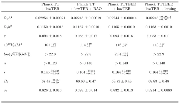
Planck TT Planck TT Planck TTTEEE Planck TTTEEE
+ lowTEB + lowTEB + BAO + lowTEB + lowTEB + lensing
Ωbh2 0.02254±0.00021 0.02243±0.00019 0.02244±0.00014 0.02245+0−0..0001400016
Ωch2 0.1150±0.0015 0.1167±0.0010 0.1165±0.0010 0.1163±0.0010
τ 0.094±0.018 0.088±0.017 0.094±0.016 0.083±0.011
1010V
0/M4 101+20−10 114 +10
−8 116 +10
−7 113 +10
−6
log(√8πb[GeV]) >22.8 >22.8 23.4+1.3
−0.8 >22.9
λ >0.128 >0.140 >0.140 >0.140
r 0.145+0−0..035018 0.164 +0.019
−0.013 0.164 +0.010
−0.018 0.164 +0.019
−0.009
H0 67.47+0−0..6579 68.68±0.47 68.72±0.48 68.83±0.48
σ8 0.826±0.015 0.828±0.014 0.832±0.013 0.8214±0.0083
Table 2. 68% c.l. constraints on cosmological parameters in our extendedΛCDM+r scenario from different combinations of datasets with a Exponential inflation.
TT + lowTEB” by the Planck collaboration. In order to check the robustness of our results, we also replace the lowTEB data with a gaussian prior on the reionization optical depth
τ = 0.055±0.009, that we call “tau055” as obtained from the Planck HFI measurements
in [11]. Afterwards, we consider the “lensing” dataset, i.e. the 2015 Planck CMB lensing
reconstruction power spectrumC`φφ[12]. Moreover, we use the "BAO" measurements. These
include the baryonic acoustic oscillation data from 6dFGS [13], SDSS-MGS [14], BOSSLOWZ
[15] and CMASS-DR11 [15] surveys as it has been done in [16]. Additionally, we consider
the CMB polarizationB modes constraints provided by the 2014 common analysis of Planck,
BICEP2 and Keck Array [17], that we call “BKP” dataset. Finally, by quoting the value
provided with direct measurements from SN1a in Riess et al. [8], we include a gaussian prior
on the Hubble constant H0= 73.2±1.7km/s/Mpc, that we call "H073p2".
In order to analyze statistically our model using these datasets, to include the corrected Exponential model, we have modified the June 2016 version of the publicly available
Monte-Carlo Markov Chain packagecosmomc[18], with a convergence diagnostic based on the Gelman
and Rubin statistic. As the original code, this version implements an efficient sampling of
the posterior distribution using the fast/slow parameter decorrelations [19], and it includes
the support for the Planck data release 2015 Likelihood Code [10] (seehttp://cosmologist.
info/cosmomc/).
4 Results: Modified Exponential Inflation
The results of our explorations are shown in Tables 2and 3, where we report the constraints
at 68% c.l. on the cosmological parameters. All the bounds that we will quote hereinafter
are at68% c.l., unless otherwise expressed. These Tables differ for the cosmological scenario
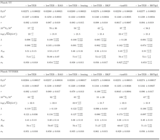
Planck TT
+ lowTEB + lowTEB + BAO + lowTEB + lensing + lowTEB + BKP +tau055 + lowTEB + H073p2
Ωbh2 0.02271±0.00022 0.02260±0.00021 0.02269±0.00021 0.02276±0.00020 0.02250±0.00020 0.02277±0.00021
Ωch2 0.1237±0.0034 0.1258±0.0033 0.1222±0.0033 0.1240±0.0034 0.1240±0.0035 0.1238±0.0034
τ 0.092±0.019 0.087±0.019 0.083±0.015 0.098±0.018 0.0617±0.0087 0.094±0.019
1010V
0/M4 57+10−30 70±30 59
+10
−40 42
+7
−20 97
+28
−15 <56.2
log(√8πb[GeV]) 22+3
−1 >21.9 >21.5 >21.4 22.4+2−1..21 >21.2
λ 0.098+0.019
−0.026 0.109−+00..028018 0.100+0−0..019029 0.085+0−0..012020 >0.126 0.091+0−0..015026
r 0.086+0.024
−0.049 0.105±0.039 0.091+0−0..025052 0.062+0−0..014029 0.162+0−0..030048 0.074+0−0..018043
Neff 3.51±0.15 3.53±0.17 3.46±0.16 3.56±0.14 3.43−+00..1517 3.55+0−0..1615
H0 71.6−+10..19 70.88±0.97 71.6 +1.2
−1.0 72.12 +0.88
−0.79 70.4 +0.8
−1.1 72.1 +1.0
−0.8
σ8 0.850±0.018 0.854+0−0..021018 0.838±0.011 0.856±0.017 0.827 +0.013
0.012 0.853
+0.17
−0.19
Planck TTTEEE
+ lowTEB + lowTEB + BAO + lowTEB + lensing + lowTEB + BKP +tau055 + lowTEB + H073p2
Ωbh2 0.02264±0.00017 0.02257±0.00016 0.02261±0.00017 0.02275±0.00016 0.02251±0.00015 0.02274±0.00017
Ωch2 0.1233±0.0027 0.1238±0.0027 0.1220±0.0026 0.1244±0.0028 0.1235±0.0026 0.1242±0.0027
τ 0.092±0.017 0.089±0.017 0.078±0.013 0.100+0.017
−0.016 0.0645±0.0084 0.096±0.017
1010V
0/M4 83+30−20 92+30−20 85−+3020 55±20 109+20−10 67+20−30
log(√8πb[GeV]) >22.3 >22.3 22.9+2.0
−0.7 >21.7 >22.3 >21.9
λ 0.119+0.024
−0.014 >0.119 0.122 +0.024
−0.011 0.096±0.018 >0.137 0.106 +0.023
−0.019
r 0.121±0.036 0.134+0.042
−0.030 0.127−+00..040033 0.080+0−0..023034 0.173+0−0..034018 0.097+0−0..033041
Neff 3.41±0.13 3.40±0.14 3.36±0.13 3.51±0.14 3.36±0.11 3.49±0.13
H0 70.4+0−1..90 70.07−+00..8196 70.4+0−1..09 71.27−+00..8877 69.67−+00..6074 71.15+0−0..9283
σ8 0.851±0.016 0.850±0.016 0.835±0.010 0.861±0.015 0.829±0.010 0.856±0.016
Table 3. 68% c.l. constraints on cosmological parameters in our extended ΛCDM+r+Neff scenario
from different combinations of datasets with a Exponential inflation.
Regarding the results of the Table2, we note that with respect to the minimal standard
cosmological model ΛCDM+r, with only 6 parameters, this modified version of the
Exponen-tial model does not improve the situation, in fact it may even provide a worse fit of the data,
increasing ∆ ¯χ2 = 9 when considering Planck TT+lowTEB, and increasing∆ ¯χ2 = 13, when
considering Planck TTTEEE+lowTEB data. As it is well known the Exponential model is
excluded from the current data since predicts a large r. We find that with the modifications
f[b, V]included, the parametersb, V0, λpreferred by data are such that the modification term
to Vef f becomes negligible. Therefore within the 6 parameter model of cosmology, the
ex-ponential model of inflation, is forced to converge towards its unmodified version, which is ruled out by data. Including our modifications to the Exponential model do not help bring it within the allowed region of best fit models.
However, there is grounds for optimism: as we now show this result does not hold in
a general ΛCDM scenario expanded beyond its minimal 6 parameter model to allow for
100 101 102 103 104
` 0
1000 2000 3000 4000 5000 6000
D
TT `[
µK
2]
Exponential LCDM
100 101
` 600
800 1000 1200 1400
D
TT `[
µK
2]
Exponential LCDM
0 500 1000 1500 2000 2500
` 20
10 0 10 20 30 40 50
D
E
E
`
[
µK
2]
Exponential LCDM
0 500 1000 1500 2000 2500
` 150
100 50 0 50 100 150
D
TE `[
µK
2]
Exponential LCDM
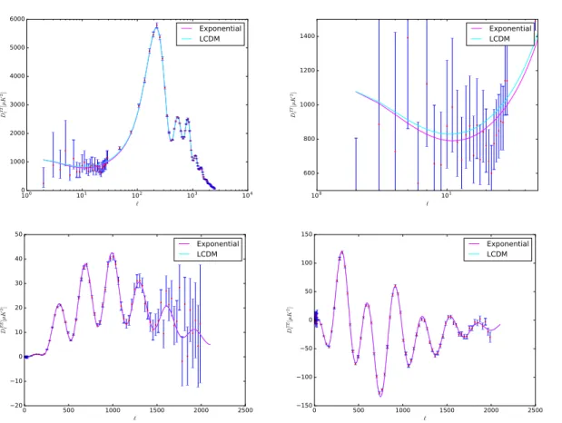
Figure 2. Comparison of the temperature and polarization CMB angular power spectra computed for the best-fit of our modified Exponential modelΛCDM+r+Neff (magenta) and the best-fit obtained
with a minimal standard cosmological model ΛCDM+r (cyan), with Planck 2015 TT+lowTEB data (points with error bars). The oly difference between the two models is at lower-`in the temperature power spectrum.
ruled out in the 6 parameter minimal standard model, we find that, also with the modifications included, the modified exponential model becomes in full agreement with Planck and SN1a data simultaneously.
And this is our important finding: from Table 3, we notice that allowing for a single
additional degree of freedom, in our case a free dark radiation component, then this model
produces a slightly better fit of the data by gaining about a ∆ ¯χ2 = 6.5, when considering
Planck TT+lowTEB, with respect to the ΛCDM+r model of the Table 2. All of this at the
price of a single additional degree of freedom to extend to a 7 parameter ΛCDM. So in
this case varying the effective number of relativistic degrees of freedom, which are degenerate
with the scalar spectral indexnS, allows the data to accommodate inflationary potentials that
are otherwise ruled out, such as the counterexample of the modified exponential inflation we analyzed in this work.
Introducing a dark radiation component Neff which is free to vary, to the modified
exponential model investigated here, where the modification are derived from the theory of the origin of the universe from the quantum landscape multiverse, we find all the cosmological
parameters with respect to ΛCDM+r model (see Table 2) shift. In particular Ωch2 shifts
3.0
3.3
3.6
3.9
N
eff
68
70
72
74
H
0
PlanckTT+lowP
PlanckTT+tau055
PlanckTTTEEE+lowP
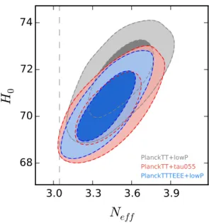
Figure 3. Constraints at 68% and95% confidence levels on the Neff vs H0 plane, in our extended
ΛCDM+r+Neff scenario. In our modified Exponential scenario, we have a robust indication at more
than2σfor an extra dark radiation component, that allows the Planck data to be in agreement with the Hubble constant value found by Riess at al. in [8].
shown in [20,21], introducing a Neff free to vary produces a value for this neutrino effective
number higher than its expected value3.045[22,23], and a shift of all the parameters that are
correlated with it. Also in our model of the modified exponential inflation, due to the strong
correlation existing between Neff and the Hubble constant H0 (see Fig. 3), by increasing the
neutrino effective number, we can relieve the tension between the constraints coming from
the Planck satellite [27] and [16] and the local measurements of the Hubble constant of Riess
at al. [28] and [8]1. For example, if we look at the results for Planck TT+lowTEB, we find
Neff = 3.51±0.15andH0 = 71.6+1−0..19, with the error bars reduced by a half with respect to the
minimal standard model. A Neff >3.045means the presence of dark radiation, that can be
explained by the existence of some extra relic component, as for example a sterile neutrino or
a thermal axion [21,24–26,31–35]. However, in contrast to the standard exponential scenario
[20,21] the constraints for our model, where the introduced modifications are derived from the
theory of the origin of the universe from the quantum landscape multiverse, are very robust.
In our case the inclusion of the high-`polarization data or the tau055 prior does not change
the constraints in a significant way with respect to Planck TT+lowTEB (see Figs. 3and 4),
even if the χ2 worsens as it happens without the modifications. Moreover, if we compute
the value of S8 =σ8
p
Ωm/0.3, we find S8 = 0.831±0.023 for Planck TT+lowTEB, which
significanlty reduces the existing tension, that becomes at 1.9σ, with KiDS-450 [36] for which
S8 = 0.745±0.039, but this increases again at2.3σ for Planck TTTEEE+lowTEB, for which
we find S8 = 0.845±0.018, as for the model without the modifications.
Since in our investigation we find a full consistency between the Planck data and the
value of the Hubble constant measured in [8], we can then safely add the priorH0 = 73.2±1.7
km/s/Mpc, to check the stability of our results. This prior confirms the results found in the
1
0.80
0.84
0.88
σ
8
68
70
72
74
H
0
PlanckTT+lowP
PlanckTT+tau055
PlanckTTTEEE+lowP
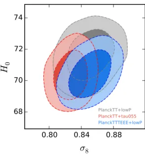
Figure 4. Constraints at 68% and 95% confidence levels on the σ8 vs H0 plane, in our extended
ΛCDM+r+Neff scenario. In our modified Exponential scenario, we don’t have the strong degeneracy
between them that is present without the entanglement corrections [21].
Planck TT+lowTEB and Planck TTTEEE+lowTEB cases, for which the S8 tension with
KiDS-450 is, respectively, at 1.8σ and 2.3σ.
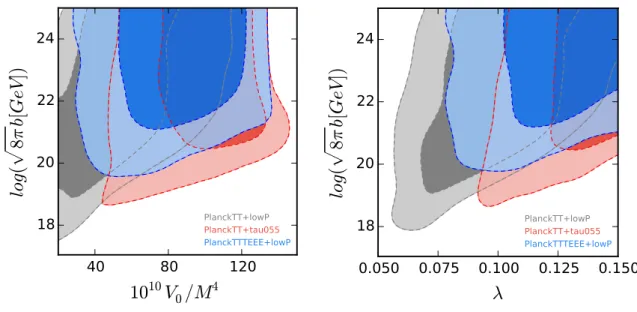
Regarding the inflationary parameters that describe the theory analyzed here, a
con-straint appears for the tensor-to-scalar ratio r, which is different from zero at more than 2
standard deviations. We find for example, that r= 0.086+0−0..024049 for Planck TT+lowTEB. In
Fig.5there are shown the constraints at68%and95%confidence levels in the1010V0/M4 vs
log(√8πb)andλvslog(√8πb)planes. We can see that the SUSY breaking scale is in between
2.6×10⁸< b <1.4×10¹⁰GeV andV0= 5.7+1−3..00×10
−9M4
P for Planck TT+lowTEB; and we
find λ= 0.098+0−0..019026.
5 Conclusions
If we insist in a 6 parameter standard model of cosmology, then the recent Planck datasets rule out convex potentials, including the exponential inflation we considered here as an illustration. This remains the case even in the presence of nonlocal modifications, like the one analyzed in this work, which is introduced by quantum entanglement in the theory of the origin of the universe from the quantum landscape. Meanwhile the friction between the findings of Planck
[16,27] and the recent SN1a measurements of the Hubble parameter of Riess et al [8] persists.
Our key finding is that if we allow for an extension beyond the 6 parameter standard
model, by introducing dark radiation Nef f > 3.045, then the exponential inflationary
po-tentials, modified by the theory analyzed here, produces a model that fits Planck datasets 2015 despite it being a convex potential, brings the Planck findings into agreement with the
SN1a results of [8] for the Hubble parameter and naturally removes the friction between these
datasets, without increasing the tension with weak lensing measurements, such as KiDS-450
[36] and CFHTLenS [37], and, for which all the predictions made from this theory in [3] for
40
80
120
10
10
V
0
/M
4
18
20
22
24
lo
g
(
p
8
π
b
[
G
eV
])
PlanckTT+lowP PlanckTT+tau055
PlanckTTTEEE+lowP
0.050 0.075 0.100 0.125 0.150
λ
18
20
22
24
lo
g
(
p
8
π
b
[
G
eV
])
PlanckTT+lowP PlanckTT+tau055
PlanckTTTEEE+lowP
Figure 5. Constraints at 68%and 95% confidence levels on the1010V
0/M4 vslog(
√
8πb) andλvs
log(√8πb)planes, in our extendedΛCDM+r+Neff scenario.
Our data analysis in the ΛCDM+r+Neff scenario, constrains, for Planck TT+lowTEB
dataset, the parameters b, λ and V0 to the following values for the 1σ and the 2σ allowed
regions respectively: 2.6×10⁸ < b < 1.4×10¹⁰GeV, λ= 0.098−+00..019026 and V0 = 5.7+1−3..00×
10−9MP4 at 68%c.l., andb >4.8×10⁷GeV,λ= 0.098−+00..040038 andV0<1.0×10⁻⁸MP4 at 95%
c.l.. The strength of modification for the 1σ value of parameters, shown in Fig. 6, is about
12%. As can be seen the modified scpetrum is more surpressed at lower multipoles than the
higher ones.
The energy modification termf(b, V)obtained from the analysis of the allowed
parame-ters for the1σ region, is up to20%of the inflaton potential for these parameters. Therefore,
the status of all the anomalies predicted in [3] as tests of this theory, are in perfect agreement
within the range observed by Planck 2015 [6]. Furthermore, as mentioned when using these
parameters to estimate the effective modified potential, we find that our model yields a ro-bust higher value for the Hubble parameter, thus removing the friction between Planck and SN1a datasets, and our model makes a robust prediction for the existence of dark radiation
Nef f = 3.51 ±0.15 at 68%c.l. which can be, for example, a light thermal axion in the form
of dark matter or a sterile neutrino species.
A key question remains: is the agreement of the modified exponential model due to the presence of additional dark radiation or is it due to the nonlocal quantum entanglement mod-ifications? A complete answer to this question would require a further comparison performed in terms of the Bayesian evidence. However, previously one of us analized the unmodified
exponential inflation in the presence of the additional dark radiation in [21], as previously
done by [20], by considering several combination of datasets. The authors found in [20] that
with additional degrees of freedom the exponential model is in agreement with the Planck
data and can solve the friction between the Planck and the SN1a [8] measurements of the
Hubble parameter H0. However, as it has been showed in [21] this extended model cannot
0.01 0.1 1 10 100 1000k 0.922
0.924 0.926 0.928
P•P0
0.01 0.1 1 10 100 1000k
1.094 1.096 1.098 1.100 1.102 1.104 1.106
Veff•V
0.01 0.1 1 10 100 1000k
0.0905 0.0910 0.0915 0.0920 r
0.01 0.1 1 10 100 1000k
0.9895 0.9896 0.9897 0.9898 0.9899 0.9900 0.9901 n
Figure 6. Shown are: the ratio of the modified spectrumP[k]over the unmodifiedP0[k]spectra;the ratio of the effective potential Vef f(φ[k])versus the unmodified exponential potentialV(φ0[k]); and
the tensor to scalar ratio r[k] and scalar index n[k], for the 1−σ parameters of this model b = 7×10⁸GeV, λ= 0.098, V
0= 5×10⁻⁹ for the modified Exponential model.
of S8, such as KiDS-450 [36] and CFHTLenS [37], and when the tau055 prior is considered,
the tension with H0 is restored. Comparing that previous analysis of the unmodified
expo-nential inflation with our very robust findings here, that do not change considering several combination of datasets, leads us to conclude that the agreement of the modified exponential inflation with all the data available, including the anomalies, the best fit region of inflationary
parameters and the Planck and SN1a data onH0 is due to the modifications. This fact makes
this model very interesting, because in a very robust way, the model fits the variety of data and can resolve the friction among various observational findings.
Acknowledgments
We would like to thank F. R. Bouchet and A. Melchiorri for stimulating discussions and we are grateful to the Planck Editorial Bord for taking the time to read the paper and approve it. This work has been done within the Labex ILP (reference ANR-10-LABX-63) part of the Idex SUPER, and received financial state aid managed by the Agence Nationale de la Recherche, as part of the programme Investissements d’avenir under the reference ANR-11-IDEX-0004-02. LMH acknowledges support from the Bahnson funds.
References
L. Mersini-Houghton, AIP Conf. Proc.861, 973 (2006) [hep-th/0512304].
[2] R. Holman and L. Mersini-Houghton, Phys. Rev. D74, 123510 (2006) [hep-th/0511102]; R. Holman and L. Mersini-Houghton, [hep-th/0512070]; L. Mersini-Houghton, AIP Conf. Proc.
878, 315 (2006) [hep-ph/0609157].
[3] R. Holman, L. Mersini-Houghton and T. Takahashi, Phys. Rev. D77, 063510 (2008) [hep-th/0611223]; R. Holman, L. Mersini-Houghton and T. Takahashi, Phys. Rev. D77, 063511 (2008) [hep-th/0612142]; L. Mersini-Houghton, arXiv:0809.3623 [hep-th];
L. Mersini-Houghton and R. Holman, JCAP0902, 006 (2009) [arXiv:0810.5388 [hep-th]]. [4] L. Mersini-Houghton, arXiv:1612.07129 [hep-th].
[5] P. A. R. Adeet al.[Planck Collaboration], “Planck 2015 results. XX. Constraints on inflation,” arXiv:1502.02114 [astro-ph.CO].
[6] P. A. R. Adeet al.[Planck Collaboration], “Planck 2015 results. XVI. Isotropy and statistics of the CMB,” arXiv:1506.07135 [astro-ph.CO].
[7] E. Di Valentino and L. Mersini-Houghton, ’Testing Predictions of the Quantum Landscape Multiverse 1: The Starobinsky Inflationary Potential’, Submitted to EPJC.
[8] A. G. Riesset al., arXiv:1604.01424 [astro-ph.CO].
[9] F. Lucchin and S. Matarrese, Phys. Rev. D32, 1316 (1985). doi:10.1103/PhysRevD.32.1316 [10] N. Aghanimet al.[Planck Collaboration], [arXiv:1507.02704 [astro-ph.CO]].
[11] N. Aghanimet al.[Planck Collaboration], arXiv:1605.02985 [astro-ph.CO]. [12] P. A. R. Adeet al.[Planck Collaboration], arXiv:1502.01591 [astro-ph.CO].
[13] F. Beutleret al., Mon. Not. Roy. Astron. Soc.416(2011) 3017 [arXiv:1106.3366 [astro-ph.CO]]. [14] A. J. Rosset al., Mon. Not. Roy. Astron. Soc.449(2015) 835 [arXiv:1409.3242 [astro-ph.CO]]. [15] L. Andersonet al. [BOSS Collaboration], Mon. Not. Roy. Astron. Soc.441(2014) 1, 24
[arXiv:1312.4877 [astro-ph.CO]].
[16] P. A. R. Adeet al.[Planck Collaboration], arXiv:1502.01589 [astro-ph.CO].
[17] P. A. R. Adeet al.[BICEP2 and Planck Collaborations], Phys. Rev. Lett.114(2015) 10, 101301 [arXiv:1502.00612 [astro-ph.CO]].
[18] A. Lewis and S. Bridle, Phys. Rev. D66, 103511 (2002) [astro-ph/0205436]. [19] A. Lewis, Phys. Rev. D87, no. 10, 103529 (2013) [arXiv:1304.4473 [astro-ph.CO]]. [20] T. Tram, R. Vallance and V. Vennin, arXiv:1606.09199 [astro-ph.CO].
[21] E. Di Valentino and F. R. Bouchet, arXiv:1609.00328 [astro-ph.CO].
[22] G. Mangano, G. Miele, S. Pastor, T. Pinto, O. Pisanti and P. D. Serpico, Nucl. Phys. B729, 221 (2005) [hep-ph/0506164].
[23] P. F. de Salas and S. Pastor, JCAP1607, no. 07, 051 (2016) [arXiv:1606.06986 [hep-ph]]. [24] A. Heavens, R. Jimenez and L. Verde, Phys. Rev. Lett.113(2014) no.24, 241302
[arXiv:1409.6217 [astro-ph.CO]];
[25] E. Di Valentino, E. Giusarma, O. Mena, A. Melchiorri and J. Silk, arXiv:1511.00975 [astro-ph.CO];
[26] M. Archidiacono, E. Giusarma, S. Hannestad and O. Mena, Adv. High Energy Phys.2013
(2013) 191047 [arXiv:1307.0637 [astro-ph.CO]].
[28] A. G. Riesset al., Astrophys. J.730(2011) 119 Erratum: [Astrophys. J.732(2011) 129] [arXiv:1103.2976 [astro-ph.CO]].
[29] E. Di Valentino, A. Melchiorri and J. Silk, arXiv:1606.00634 [astro-ph.CO].
[30] Q. G. Huang and K. Wang, Eur. Phys. J. C76, no. 9, 506 (2016) [arXiv:1606.05965 [astro-ph.CO]].
[31] E. Di Valentino, E. Giusarma, M. Lattanzi, O. Mena, A. Melchiorri and J. Silk, Phys. Lett. B
752, 182 (2016) doi:10.1016/j.physletb.2015.11.025 [arXiv:1507.08665 [astro-ph.CO]].
[32] E. Di Valentino, S. Gariazzo, M. Gerbino, E. Giusarma and O. Mena, Phys. Rev. D93, no. 8, 083523 (2016) doi:10.1103/PhysRevD.93.083523 [arXiv:1601.07557 [astro-ph.CO]].
[33] E. Giusarma, E. Di Valentino, M. Lattanzi, A. Melchiorri and O. Mena, Phys. Rev. D90, no. 4, 043507 (2014) doi:10.1103/PhysRevD.90.043507 [arXiv:1403.4852 [astro-ph.CO]].
[34] E. Di Valentino, A. Melchiorri and O. Mena, JCAP1311, 018 (2013) doi:10.1088/1475-7516/2013/11/018 [arXiv:1304.5981 [astro-ph.CO]].
[35] M. Archidiacono, E. Calabrese and A. Melchiorri, Phys. Rev. D84, 123008 (2011) doi:10.1103/PhysRevD.84.123008 [arXiv:1109.2767 [astro-ph.CO]].
[36] H. Hildebrandtet al., arXiv:1606.05338 [astro-ph.CO].
![Figure 6. Shown are: the ratio of the modified spectrum P [k] over the unmodified P 0[k] spectra;the ratio of the effective potential V ef f (φ[k]) versus the unmodified exponential potential V (φ 0 [k]); and the tensor to scalar ratio r[k] and scalar inde](https://thumb-us.123doks.com/thumbv2/123dok_us/8295594.2196870/14.892.139.772.120.537/modified-spectrum-unmodified-effective-potential-unmodified-exponential-potential.webp)
