TSClust Approach Using K-Means Method to Forecast Vegetable Food Commodities Inflation in DKI Jakarta

TSClust Approach Using K-Means Method to Forecast

Vegetable Food Commodities Inflation in DKI Jakarta

Emeylia Safitri*_{, I Made Sumertajaya}*_{, Muhammad Nur Aidi} * * _{Department of Statistics, IPB University}

DOI: 10.29322/IJSRP.9.09.2019.p9357

http://dx.doi.org/10.29322/IJSRP.9.09.2019.p9357

Abstract- Forecasting is used to measure uncertainty based on past information from a variable called a time series. One method for forecasting by modeling is Autoregressive Integrated Moving Average (ARIMA). In one case, when forecasting is done for many dependent variables, then modeling with ARIMA directly will produce many models so that it becomes inefficient. The clustering time series approach as pre-processing can be done with

K-Means methods. Individual level modeling is important because

this method requires the same dimensions for each object. Approach I is to model the object using the original model, while approach II is to model the object with the AR (p) model. Approach I produces the value of Sw / Sb and RMSE lower than approach II. That means approach I produces a cluster and a cluster level model that is better than approach II.DKI Jakarta's vegetable food commodities are clustered into 4 groups based on the results of K-Means with I approach which is the optimal group. Each group has a different model.

Index Terms: ARIMA, clustering time series, modelling, K-Means

method, inflation of vegetable food commodities DKI Jakarta

I. INTRODUCTION

National inflation is a reflection of regional inflation [1]. Monthly inflation of DKI Jakarta from 2012-2017 has a fluctuating pattern and is similar to the national inflation pattern. DKI Jakarta has an inflation weight of 20.15% of the national inflation [2]. It is the biggest weight compared to other cities in Indonesia, thus making this region the critical area of national inflations.

The foodstuffs group in DKI Jakarta often contributed significantly to inflation compared to other groups. Until 2017, the foodstuffs group experienced a fluctuating contribution but continued to dominate. One commodity that is always a concern in inflation from the foodstuffs group is agricultural food commodities. Food commodities from the agricultural sector often play an important role in inflation in DKI Jakarta such as red chili, shallots and others.

Forecasting the amount of commodity inflation included in the foodstuff category is becoming quite important. That is because commodities from the agricultural sector are related to food, which is a basic need for human resources. One of the method for forecasting using modeling is Autoregressive Integrated Moving Average (ARIMA) [3]. The ARIMA model uses the past and present values of a dependent variable to produce an accurate

For a time series data, the ARIMA model will produce a model that is used for forecasting. In one case, when forecasting is done for many dependent variables in the form of time series, and then modeling with ARIMA will directly produce many models. Direct ARIMA modeling for dependent variables becomes inefficient and ineffective. Handling of these problems is using the TSClust approach as pre-processing. Previous research by Utami [5] conducted the TSClust approach as pre-processing for forecasting the magnitude of inflation in sub-commodities in DKI Jakarta. Based on some studies the TSClust approach produces a cluster level model that is not much different from the individual level modeling of forecasting results.

One simple cluster analysis that can be used is K-Means [6]. There are two approaches taken for parameter preparation such as approach I with the original model and approach II with the AR (p) model [7]. Therefore, this study aims to forecast the inflation of Jakarta's vegetable food commodities using the K-Means method as pre-prosessing.

II. MATERIALS AND METHODS

2.1 Data

The real data used is sourced from the DKI Jakarta BPS publications, the Jakarta Consumer Price Index and Inflation. The real data that will be processed in this study is the monthly inflation data for DKI Jakarta vegetable food commodities from January 2012 to December 2018.

2.2 Data Analysis Procedure

The steps of analysis will be by the following: 1. Data Exploration

Data exploration was conducted on the real data of monthly inflation of agricultural food commodities in 2012-2018. At this stage, time series data movement patterns will be identified for each commodity.

2. Dividing data

The data divided into training data and test data. The data will be divided into 2 (two), which is 78 training data (January 2012-June 2018) and 6 test data (July 2018-December 2018). 3. Individual modeling for commodities is done by two

This process begins with checking the data stationarity, such as:

i. Examine the plot of time series data.

ii. Perform an Augmented Dickey-Fuller (ADF) test.

b. Estimating parameters.

Estimating the parameters of the ARIMA model. This step is carried out on all candidate models. In addition, the candidate model Bayesian information Criterion (BIC) value will be obtained with the following equation:

𝐵𝐵𝐵𝐵𝐵𝐵=−2 𝑙𝑙𝑙𝑙 (𝐿𝐿) +𝑘𝑘 ln (𝑙𝑙) (1)

With,

L = maximum value of the likelihood function; n = number of observations; k = p + q + 1, if the model contains the term intercept and k = p + q if otherwise, where p represents the number of parameters of the AR (p) model and q is the number of parameters for the MA (q) model.

c. Testing the residuals models obtained.

4. Compile data containing paremeters and variance-covariance matrix for all 43 commodities. Parameters preparation with approach I is illustrated in Table 1.

Table 1: Ilustration of parameters preparation with approach I (original model)

Objek Model Parameter

ф1 ф2 ... θ1 θ2 ... 1 AR(2) 0.8 0.2 0 0 0 0

2 MA(1) 0 0 0 0.4 0 0

... ... .... ... ... ... ... ...

5. Clustering time series with the K-Means method and calculate the value of Sw / Sb for values k = 2 to k = 10. Sw is the average standard deviation within the cluster; Sb is the average standard deviation between the clusters [8].

6. Identifying the optimum stable number of cluster based on Sw / Sb values.

7. Calculating cluster representatives.

Forming the average from t = 1 to t = 78 (number of series) [9].

8. Perform cluster level modelling with prototype. The steps are the same as stage 3.

9. Calculating RMSE to select the optimum number of clusters by forecasting using test data with the best model on each cluster.

10. Forecasting with cluster level model.

III. RESULTS

3.1 Explorating of DKI Jakarta Vegetable Food Commodity Inflation Data

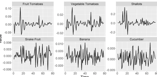
Plot of time series data was carried out to examine the patterns of inflation in Jakarta's vegetable food commodities. The time series plot of some vegetable food commodities is presented in Figure 1. The inflation pattern of shallot commodities is seen to fluctuate until the 40th period marked by a significant increase and decrease. After the 40th period, these commodities tend to be more stable although they remain fluctuative. The same pattern with shallots commodities appear on vegetable tomatoes and fruit tomatoes, although with a different range of inflation values. Banana commodities appear to be fluctuative in all times. Some commodities have a similar pattern to banana commodities, such as bark and cucumber. The three commodities have fluctuating patterns from the beginning to the end of the period. Similar patterns between commodities can be used as an indication that the commodity can be clustered into the same cluster in the cluster analysis.

Figure 1: Plot of inflation in several DKI Jakarta vegetable food commodities

Table 1 presents descriptive statistics of commodities, which have a large standard deviation and are greater than the average value. A large deviation indicates various inflation values. The red chili commodity (Y41) has a higher standard deviation value than other commodities. This means that the value of inflation produced is more diverse than other commodities. The commodities in Table 1 have experienced deflation based on the minimum value of inflation produced, which has a negative sign.

Table 1: Several commodities with large standard deviation values

Obs. Mean Median Sd Min Max Y41

Y28 Y1 Y36

Y3

0.002 0.005 0.022 0.010 0.003

0.006 0.006 0.004 0.003 0.002

0.072 0.015 0.054 0.073 0.012

-0.270 -0.043 -0.129 -0.252 -0.023

3.2 Select tthe Optimum Number of Cluster

Figure 2: Comparison of the Sw / Sb value of the K-Means method with two approaches

K-Means method requires the initial of the number of cluster (k). Figure 2 presents a comparison of Sw / Sb for the K-Means method with two approaches. Both approaches produce almost the same pattern, which is the pattern decreases with increasing number of groups (k). The value of Sw / Sb with the AR (p) approach looks sloping; the original model approach has a steeper Sw / Sb pattern due to a large decrease in value. The decrease is seen on the way to k = 3. Therefore, the chosen k value is from k = 4 to k = 7 Next, the optimum k value will be chosen based on the minimum RMSE value.

3.3 Cluster level modeling

The selection of the number of cluster (k) is determined from the average minimum RMSE value. Table 2 presents the average RMSE values for several k values. The RMSE value is the average of the RMSE of all groups. The RMSE values generated by the two approaches do not differ greatly. In approach I (original model) the lowest average RMSE is 0.012, while for approach II (AR (p)) is 0.026. Overall the RMSE value generated by approach I is lower than approach II. Based on the minimum RMSE value, the optimum cluster produced are 4 groups with approach II, namely the original model with the lowest BIC criteria.

Table 2: Comparison of RMSE values in cluster level models

Number of Clusters (k)

Average RMSE Original model (I) AR(p) (II)

4 0.012 0.039

5 0.033 0.035

6 0.030 0.030

7 0.026 0.026

8 0.023 0.027

3.4 Identification of Optimum Cluster

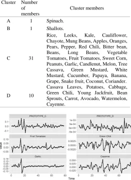
Table 3 presents member details for optimum cluster results. Commodities in one cluster have the same inflation movement pattern. Forecasting the amount of inflation in objects that are in one cluster will be the same value. Figure 3 presents the inflation movement patterns for the optimum cluster prototype and several objects that are in one cluster.

Table 3: Optimal cluster member details

Cluster Number of members

Cluster members

A 1 Spinach.

B 1 Shallots.

C 31

Rice, Leeks, Kale, Cauliflower, Chayote, Mung Beans, Apples, Oranges, Pears, Pepper, Red Chili, Bitter bean, Beans, Long Beans, Vegetable Tomatoes, Fruit Tomatoes, Sweet Corn, Peanuts, Garlic, Candlenut, Melon, Tree Cassava, Green Mustard, White Mustard, Cucumber, Papaya, Banana, Grape, Snake fruit, Coconut, Coriander.

D 10

Cassava Leaves, Potatoes, Cabbage, Green Chili, Young Jackfruit, Bean Sprouts, Carrot, Avocado, Watermelon, Cayenne.

Figure 3: Plot prototype of the optimum cluster and several objects in the same cluster

Group C has the most members, which is 31 objects. There are rice, red chili, and garlic. These commodities often experience price changes. The prototype inflation pattern in cluster C is presented in Figure 3. In periods 0 to 20, inflation patterns seen fluctuated, while the next period seen more stable. Group D consists of 10 commodities, the resulting inflation pattern seen more fluctuated from the beginning to the end of the period; there is no decrease or an extreme increase. Green chili and cayenne have the same pattern with prototype D.

(a)

(b)

Figure 4: : Prototype plot with fitting ARIMA models on cluster A (a) and cluster B (b)

Table 4: Details of optimum cluster models

Cluster Model Equation model Uji ADF

A _ARIMA(0,1,0) ∇Yt = et 0.164

B ARIMA(0,0,1) Yt = -0.45et-1 + et 0.010 C ARIMA(0,1,0)* ∇Yt = 0.006 + et 0.138 D _ARIMA(0,1,1) ∇Yt = -0.954et-1 + et _0.139

*: Model has intersept>0

The ARIMA level of cluster at the optimum number of clusters (k) is presented in Table 4. The resulting cluster level models vary. Cluster C has a model with intercept not equal to zero. This means that the intercept value affects the forecast results. Cluster A and C have the same model which is ARIMA (0,1,0). However, cluster C has an interception > 0. Figure 4 presents a prototype plot with a cluster-level ARIMA fitted model. Cluster A and C have the same prototype pattern as the results of the ARIMA fitted model. This means that the built model is sufficient to represent the prototype pattern. The resulting fitted ARIMA model looks underestimated. This means that the alleged value of the model is lower than the prototype. However, several periods result in the overestimated value of the fitted ARIMA model, which is when the inflation value on the prototype decreases considerably.

3.5 Application of cluster-level ARIMA models

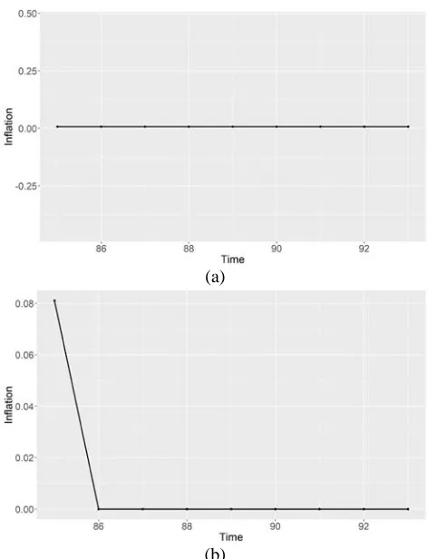
(a)

(b)

Figure 5: Forecasting 9 periods in cluster A (a) and cluster B (b)

Figure 5 presents the forecasting results for several clusters. Cluster A is an ARIMA model (0,1,0) with an intercept of zero, so that the resulting forecast is zero for the whole period. Cluster B has the ARIMA model (0,0,1). Forecasting value resulting only in the first period, for the next period has a forecast value of intercept (average), which is zero.

IV. CONCLUSION

The K-Means method with 2 approaches in constructing individual models produces a cluster result that does not differ much. This is based on the value of Sw / Sb and the resulting RMSE. Vegetable food commodities are grouped into 5 clusters. Most of the commodities cluster in cluster C. The models produced in each clusters are different.

ACKNOWLEDGEMENTS

This work is fully supported by Kemenristek DIKTI (Kementerian Riset Teknologi dan Pendidikan Tinggi) of Indonesia.

REFERENCES

[1] [BI] Bank Indonesia. Statistik Ekonomi Keuangan

[2] [BPS Jakarta] Badan Pusat Statistik DKI Jakarta. Indeks

Harga Konsumen dan Inflasi DKI Jakarta. Jakarta : BPS

DKI Jakarta. 2015.

[3] Wei WWS. Time Series Analysis,Univariate and

Multivariate Methods, Second Edition. New York (US):

Pearson Education, Inc. 2006.

[4] Montgomery DC, Jennings CL, Kulahci M. Introduction

To Time Series Analysis And Forecasting. New Jersey:

John Wiley & Sons. Inc. 2008.

[5] Utami B. Time-Series Data Modelling for Inflation Forecasting based on Subcategories of Comodity using TSClust Approach as Pre-processing. J. Sciences. vol.39, no.2, pp. 21-23, 2018.

[6] Mattjik AA, Sumertajaya IM. Sidik Peubah Ganda dengan Menggunakan SAS. Bogor (ID) : IPB Press. 2011. [7] Piccolo D. A Distance Measure For Classifying ARIMA

Models. J. doi:10.1111/j.1467-9892.1990.tb00048 x.

vol.11, no.2, pp. 153-164, 1990.

[8] Kalkstein LS, Tan G, dan Skindlov JA. An evaluation of three clustering procedures for use in synoptic climatological classification. J. climate and applied

meteorology. vol.26, no.2, pp. 717-730, 1987.

[9] Aghabozorghi S, Shirkhorsidi AS, Wah TY. 2015. Time-Series clustering Adecade review. J. Information Systems. doi:10.1016/j.is.2015.04.007.

AUTHORS

First Author – Emeylia Safitri S. Stat, college student,

Department of Statistics, Faculty of Mathematics and Natural Sciences (FMIPA), IPB University, Bogor,16680, Indonesia, and [email protected]

Second Author – Dr. Ir. I Made Sumertajaya, MS, Lecturer,

Departement of Statistics, Faculty of Mathematics and Natural Sciences (FMIPA), IPB University, Bogor,16680, Indonesia, and [email protected]

Third Author – Dr. Ir. Muhammad Nur Aidi, M.S, Lecturer,

Department of Statistics, Faculty of Mathematics and Natural Sciences (FMIPA), IPB University, Bogor,16680, Indonesia, and [email protected]

Correspondence Author - Dr. Ir. I Made Sumertajaya, MS, Lecturer, Department of Statistics, Faculty of Mathematics and Natural Sciences (FMIPA), IPB University, Bogor,16680, Indonesia, and