Estimations of Weibull Geometric Distribution under Progressive Type II Censoring Samples

http://dx.doi.org/10.4236/ojs.2015.57072

Estimations of Weibull-Geometric

Distribution under Progressive Type II

Censoring Samples

Azhari A. Elhag1, Omar I. O. Ibrahim2, Mohamed A. El-Sayed3,4, Gamal A. Abd-Elmougod1 1_{Department of Mathematics, Faculty of Science, Taif University, Taif, Saudi Arabia}

2_{Department of Mathematics, Faculty of Science, Taif University, Ranyah Branch, Saudi Arabia} 3_{Department of Mathematics, Faculty of Science, Fayoum University, Al Fayoum, Egypt}

4_{Department of Computer Science, College of Computer and IT, Taif University, Taif, Saudi Arabia}

Received 23 October 2015; accepted 15 December 2015; published 18 December 2015

Copyright © 2015 by authors and Scientific Research Publishing Inc.

This work is licensed under the Creative Commons Attribution International License (CC BY).

http://creativecommons.org/licenses/by/4.0/

Abstract

This paper deals with the Bayesian inferences of unknown parameters of the progressively Type II censored Weibull-geometric (WG) distribution. The Bayes estimators cannot be obtained in expli-cit forms of the unknown parameters under a squared error loss function. The approximate Bayes estimators will be computed using the idea of Markov Chain Monte Carlo (MCMC) method to gen-erate from the posterior distributions. Also the point estimation and confidence intervals based on maximum likelihood and bootstrap technique are also proposed. The approximate Bayes esti-mators will be obtained under the assumptions of informative and non-informative priors are compared with the maximum likelihood estimators. A numerical example is provided to illustrate the proposed estimation methods here. Maximum likelihood, bootstrap and the different Bayes estimates are compared via a Monte Carlo Simulation study.

Keywords

Weibull-Geometric Distribution, Progressive Type II Censoring Samples, Bayesian Estimation, Maximum Likelihood Estimation, Bootstrap Confidence Intervals, Markov Chain Monte Carlo

1. Introduction

in medical, biological and engineering sciences. Some applications of the Weibull distribution in forestry are given in Green et al. [1]. Several distributions have been proposed in the literature to extend the Weibull distri-bution. Adamidis and Loukas [2] introduce the two-parameter exponential-geometric (EG) distribution with de-creasing failure rate. Marshall and Olkin [3] present a method for adding a parameter to a family of distributions with application to the exponential and Weibull families. Adamidis et al. [4] introduce the extended exponen-tial-geometric (EEG) distribution which generalizes the EG distribution and discuss variety of its statistical properties along with its reliability features. The hazard function of the EEG distribution can be monotone de-creasing, increasing or constant. Kus [5] proposes the exponential-Poisson distribution (following the same idea of the EG distribution) with decreasing failure rate and discusses its various properties. Souza et al[6] introduce the Weibull-geometric (WG) distribution that contains the EEG, EG and Weibull distributions as special sub- models and discuss some of its properties. For more details about Weibull-geometric (WG) distribution and its properties, see Barreto-Souza [7] and Hamedani and Ahsanullah [8].

Let X follows a WG distribution, then the probability density function (pdf) f x

( )

and distribution function (cdf) F x

( )

of WG distribution are given respectively by

( )

(

)

(

( )

)

( )

(

)

1 2 1 exp

, 0, , 0 and 1

1 exp

p x x

f x x p

p x α α α α αβ β α β β − − −

= > > <

 _{− −}      (1) and

( )

(

( )

)

( )

(

)

1 exp 1 exp x F x p x α α β β − − =

− − (2)

Some special sub-models of the WG distribution (1) are obtained as follows. If p=0, we have the Weibull distribution. When p→1, the WG distribution tends to a distribution degenerate in zero. Hence, the parameter p can be interpreted as a concentration parameter. The EG distribution corresponds to α =1 and 0< <p 1, whereas the EEG distribution is obtained by taking α =1 for any p<1. Clearly, the EEG distribution extends the EG distribution. WG density functions are displayed. For − ≤ <1 p 1, the WG density is unimodal if α >1 and strictly decreasing if α ≤1. The mode x0 1 1u

α

β−

= is obtained by solving the nonlinear equation

( )

1 1 1

exp

u p u u α α

α α

−  −  −

+ _ + _=

  (3) For p< −1, the WG density can be unimodal. For example, the EEG distribution (α =1) is unimodalif

1

p< − .

The survival and hazard functions of X are

( )

(

)

(

( )

)

( )

(

)

1 exp , 1 exp p t S t p t α α β β − − =

− − (4)

and

( )

(

)

( )

(

)

1 1 1 exp p t h t p t α α α αβ β − − =

− − (5)

Suppose that n independent items are put on a life test with continuous identically distributed failure times

1, 2, , n

X X  X . Let further that a censoring scheme

(

R R1, 2,,Rm

)

is previously fixed such that immediately following the first failure X1, R1 surviving items are removed at random from the test, after the next failure

2

X , R2 surviving items are removed at random from the test; this process continues until, at the time of the

m-th observed failure Xm, the remaining Rm items are removed from the test. The m is ordered observed fail-ure times denoted by X1,m,X2,m,,Xm m,

R R R

proba-bility density function for X1,m,X2,m,,Xm m,

R R R

is given (see Balakrishnan and Sandhu [9]) by

(

)

(

)

(

)

1,2, , 1; , 2; , ; , ; , ; ,

1

1; , 2; , ; ,

, , , 1 ,

0 ,

i

m _R

m m n m n m m n i m n i m n i

R R R

m n m n m m n

f x x x C f x F x

x x x

=

 

= _ − _

< < < < < ∞

∏

 



R R R R R

(6)

where

(

1 1

)(

1 2 2

)

(

1 2 m 1 1 .

)

C=n n−R − n−R −R −  n−R −R − − R − − −m (7)

Progressive Type II censored sampling is an important scheme of obtaining data in lifetime studies. For more details on the progressive censored samples see Aggarwala and Balakrishnan [10].

2. Markov Chain Monte Carlo Techniques

MCMC methodology provides a useful tool for realistic statistical modeling (Gilks et al. [11]; Gamerman, [12]), and has become very popular for Bayesian computation in complex statistical models. Bayesian analysis re-quires integration over possibly high-dimensional probability distributions to make inferences about model pa-rameters or to make predictions. MCMC is essentially Monte Carlo integration using Markov chains. The inte-gration draws samples from the required distribution, and then forms sample averages to approximate expecta-tions (see Geman and Geman, [13]; Metropolis et al., [14]; Hastings, [15]).

Gibbs Sampler

The Gibbs sampling algorithm is one of the simplest Markov chain Monte Carlo algorithms. It was introduced by Geman [13]. The paper by Gelfand and Smith [16] helped to demonstrate the value of the Gibbs algorithm for a range of problems in Bayesian analysis. Gibbs sampling is a MCMC scheme where the transition kernel is formed by the full conditional distributions.

The Gibbs sampler is applicable for certain classes of problems, based on two main criterions. Given a target distribution g

( )

Θ , where Θ =

(

θ θ θi 1, 2,,θd

)

, The first criterion is 1) that it is necessary that we have an analytic (mathematical) expression for the conditional distribution of each variable in the joint distribution given all other variables in the joint. Formally, if the target distribution g

( )

Θ is d-dimensional, we must have d in- dividual expressions for g

(

θ θ θi| 1, 2,;θ θi−1, i+1,,θd

) (

=g θ θi| j

)

,i≠ j.

Each of these expressions defines the probability of the i-th dimension given that we have values for all other (i≠ j) dimensions. Having the conditional distribution for each variable means that we don’t need a proposal distribution or an accept/reject criterion, like in the Metropolis-Hastings algorithm. Therefore, we can simply sample from each conditional while keeping all other variables held fixed. So that we must be able to sample from each conditional distribution if we want an implementable algorithm.

To define the Gibbs sampling algorithm, let the set of full conditional distributions be

(

) (

)

(

)

{

g θ θ θ1| 2, 3,,θd ;g θ θ θ2| 1, 3,,θd ;;g θ θ θd| 1, 2,,θd−1

}

.

Now one cycle of the Gibbs sampling algorithm is completed by simulating

{ }

θk dk=₁ from these distributions, recursively refreshing the conditioning variables.

Algorithm:

1) Choose an arbitrary starting point θ( )0 =

(

θ1( )0 ,,θd( )0

)

for which

( )

( )

0

0 g θ > ;

2) Obtain 1( )

t

θ from conditional distribution

(

1| 2( )1, 3( )1, , ( )1

)

t t t d g θ θ − θ − θ − ;

3) Obtain 2( )

t

θ from conditional distribution

(

2| 1( ), 3( )1, , 1( )1

)

t t t

g θ θ θ − θ − ;

4) Obtain θd( )t from conditional distribution

( ) ( ) ( ) ( )

(

| 1 , 2 , 3 , , 1

)

t t t t

d d

g θ θ θ θ θ − ;

5) Repeat of steps 2 - 4 thousands (or millions) of times for the number of samples M.

The results of the first M or so iterations should be ignored, as this is a “burn-in” period for the algorithm to set itself up.

for the three unknown parameter of WG distribution. In Bayesian technique, we use the idea of Markov chain Monte Carlo (MCMC) techniques to generate from the posterior distributions. Finally, we will give an example to illustrate our proposed method.

3. Maximum Likelihood Estimation

Let Xi =Xi m n; ,

R

, i=1, 2,, ,m be the progressive first-failure censored order statistics from a Weibull-geometric

distribution, with censored scheme R, where n independent items are put on a life test with continuous identi-cally distributed failure times X X1, 2,,Xn. Suppose further that a censoring scheme

(

R R1, 2,,Rm

)

is pre-viously fixed. From (1), (2) and (3), the likelihood function is given by

(

)

(

)

(

)

(

)

(

)

(

)(

)

1 2 1 1 1

; , , 1 exp 1 ,

1 exp i i R m m m i m m i i R i i i p x

L x p p R x

p x

α

α α

α

α β α β β

β − + = =    −    ∝ − _{  }− + _      _{− −}   _{ }   

∏

∑

(8)

where C is given by (7). The logarithm of the likelihood function l may then be written as

(

)

( )

(

) (

)

(

)

(

(

(

)

)

)

(

)(

)

1

1 1

; , , 1 1 log

2 log 1 exp 1 .

m

i i

m m

i i i i

i i

l x p mLog nLog p x

R p x R x

α

α α

α β αβ α

β β = = = = + − + − − + − − − +

∑

∑

∑

(9)

Calculating the first partial derivatives of (9) with respect to α β, and p equating each to zero, we get the likelihood equations as in the following:

(

)

(

)

(

)

(

(

)

)

(

)

(

)

(

)(

)

(

)

1 1 1

2 log exp

; , ,

log log

1 exp

1 log ,

m m _{i i i}

i

i i

i

m

i i i

i

R x x

l x p m

x p

p x

R x x

α α

α

α

β β β

α β

β

α α _β

β β = = = + − ∂ = + + − ∂ _{− −} − +

∑

∑

∑

(10)

(

)

(

)

( )

(

( )

)

( )

(

)

(

)

( )

1 1 1 2 exp ; , , 2 , 1 exp

m _{i i i} m

i i

i i

i

R x x

l x p m

p R x

p x α α α α α α αβ β

α β α _αβ

β β _β

−

= =

+ −

∂

= − − +

∂

∑

_{− −}

∑

(11)

and

(

)

(

( )

)

( )

(

)

1 1 exp ; , , ,

1 _{1 exp}

m _i

i

i x

l x p n

p p _{p x}

α α β α β β − = − ∂ ₌ − ₊

∂ −

∑

_{− −} (12)

Since (10-12) cannot be solved analytically for α βˆ, ˆ and ˆp, some numerical methods such Newton’s me-thod must be employed.

Approximate confidence intervals for α β, and p can be found by to be bivariately normal distributed with mean

(

α β, ,p

)

and covariance matrix 1

(

)

0 ˆ, ,ˆ ˆ

I− α β p . Thus, the 100 1

(

−α

)

% approximate confidence inter-vals for α β, and p are

(

2 11 2 11

) (

2 22 2 22

) (

2 33 2 33

)

ˆ ˆ

ˆ zα v ,ˆ zα v , zα v , zα v and ˆ zα v ,ˆ zα v

α− α+ β− β+ α− α+ (13)

respectively, where v11, v22 and v33 are the elements on the main diagonal of the covariance matrix

(

)

1 0 ˆ, ,ˆ ˆ

I− α β p and

2

zα is the percentile of the standard normal distribution with right-tail probability 2 α .

4. Bootstrap Confidence Intervals

inter-vals, but it can also be used to estimate bias and variance of an estimator or calibrate hypothesis tests. In this section, we use the parametric bootstrap percentile method suggested by Efron [17][18] to construct confidence intervals for the parameters. The following steps are followed to obtain progressive first failure censoring boot-strap sample from Weibull-geometric distribution with parameters α βˆ, ˆ and ˆp based on simulated progres-sively first-failure censored data set.

Algorithm:

• From an original data set 1; , , , 2; , , , , ; , ,

R R R m n k m n k m m n k

x≡x x  x , compute the ML estimates of parameters α βˆ, ˆ and ˆp from Equation (9) and Equation (10);

• Use α βˆ, ˆ and ˆp to generate a bootstrap sample x∗ with the same values of Ri,

(

i=1, 2,,m

)

using the algorithm of Balakrishnan and Sandhu [2];

• As in step 1 based on x∗ compute the bootstrap sample estimates of α βˆ, ˆ and ˆp say α βˆ ,∗ ˆ∗ and ˆp∗; • Repeat steps 2 - 3 N times representing N bootstrap MLE’s of α βˆ, ˆ and ˆp based on N different bootstrap

samples;

• Arrange all α βˆ ,∗j ˆ∗j

and ˆp∗j in an ascending order to obtain bootstrap sample

(

ϕ ϕ_t[ ]1, [ ]_t2,,ϕ_t[ ]N

)

, 1, 2, 3

t= where (ϕ α1 ˆ , ∗

= ϕ2 βˆ ,

∗

= ϕ3 pˆ

∗ = );

• Let G z

( )

=P

(

ϕt <z

)

be cumulative distribution function of ϕt; • Define ϕtboot G 1

( )

z

−

= for given z. The approximate bootstrap 100

(

1−γ

)

% confidence interval of ϕt given by

, 1 .

2 2

tboot tboot

γ γ

ϕ ϕ

    ₋ 

   

 _{   }

  (14)

5. Bayesian Estimation Using MCMC

In this section, we consider the Bayes estimation of the unknown parameter(s). In many practical situations, the information about the parameters are available in an independent manner. Thus, here it is assumed that the pa-rameters are independent a priori and assumed that α and β have the following gamma prior distributions

( )

1

(

)

1 exp ,

a

b

π α _∝α − ₋ α

(15)

( )

1

(

)

2 exp .

c

d

π β _∝β − ₋ β

(16)

Here all the hyper parameters a, b, c, d are assumed to be known and non-negative and let the NIP for para-meter p which represented by the limiting form of the appropriate natural conjugate prior, the NIP for the acce-leration factor p is given by

( )

1

3 p p , p 0.

π ₌ − _>

(17)

Therefore, the joint prior of the three parameters can be expressed by

(

)

1 1 1

(

)

, ,p a c p exp b d , , , p 0.

π α β _∝α β− − − ₋ α₋ β α β _>

(18)

Therefore, the Bayes estimate of any function of α β, and p say ϕ α β

(

, ,p

)

, under squared error loss func-tion (SEL) is

(

)

, , |

(

(

)

)

ˆ , ,p Eα β p x , ,p .

ϕ α β = ϕ α β (19)

The MCMC method to generate samples from the posterior distributions and then compute the Bayes estima-tor of ϕ α β

(

, ,p

)

under the SEL function.

posterior distribution. This is also true of any function of the parameters.

When practically possible, we give prior and posterior distributions in terms of known densities, such as the Gaussian, binomial, beta, gamma and others. The joint posterior density function of α β, and p can be ob-tained by multiply the likelihood function (multivariate normal) with the prior which can be written as:

(

)

(

)

(

)

(

)

(

)( )

( )

(

)

1 1 1 2 1 1

, , | 1 1 exp exp

exp 1 .

1 exp i

n a m c m

m m

i

i i R

i i

i

p x p p b d

x R x p x α α α α

π α β α β α β

β β ∗ + − + − − + = = ∝ − − − −       × _− + _×    _  _{− −}  _      

∑

∏

(20)

We obtain the Bayes MCMC point estimate of ϕ_l (ϕ₁=α, ϕ2 =β and ϕ =3 p) as

(

)

( ) 1 1 | , N i l l i M E x N M ϕ ϕ = + =

−

∑

(21)

where M is the burn-in period (that is, a number of iterations before the stationary distribution is achieved), and posterior variance of ϕl becomes

(

)

(

( )

₍

₎

)

2

1 1

ˆ _| N i ˆ _{| ,}

l l l

i M

V x E x

N M

ϕ ϕ ϕ

= +

= −

−

∑

(22)

6. Illustrative Example

To illustrative the estimation techniques developed in this article, for given hybrid parameters

(

a=1.5,b=1

)

generate random sample of size 10, from gamma distribution the mean of the random sample

10

1 1 10i i

α α

= ≅

_∑

, is

computed and considered as the actual population value of α =1.5. That is, the prior parameters are selected to

satisfy E

( )

b a

α = ≅α, that is approximately the mean of gamma distribution (21). Also for given values

(

c=2,d=1

)

, generate according the last β =2, from gamma distribution. The prior parameters are selected to

satisfy E

( )

d c

β = ≅β, that is approximately the mean of gamma distribution. We have considered a progressive

Type II sample is generated from WG distribution with parameters (α =1.5, β =2, p=0.5, n=50, 50

[image:6.595.115.533.140.253.2]

m= and R=

{

2, 0, 2, 0,1, 0, 2, 0, 0, 3, 0, 0, 2, 0, 2, 0,1, 0, 3, 0, 3, 0, 2, 0, 2

}

) using the algorithm of Balakrishnan and Sandhu [9], the data given in by: 0.0212, 0.0463, 0.0568, 0.0686, 0.0764, 0.0832, 0.0933, 0.1031, 0.1496, 0.1485, 0.1511, 0.1536, 0.1603, 0.1685, 0.1985, 0.2097, 0.2176, 0.2643, 0.2696, 0.2809, 0.3156, 0.3744, 0.3941, 0.4196, 0.5236.

Table 1.Different estimates of parameters of WG distribution.

Parameters Method

(.) ML (.) Boot (.) MCMC

1.5

α= 1.5896 1.9026 1.5996

2.0

β = 1.8969 2.4043 1. 9069

0.5

p= 0.4754 0.8028 0.4905

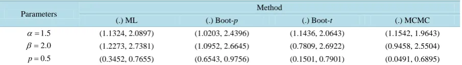
Table 2. MLE, percentile bootstrap CIs and Bootstrap-t CIs based on 500 replications.

Parameters Method

(.) ML (.) Boot-p (.) Boot-t (.) MCMC

1.5

α = (1.1324, 2.0897) (1.0203, 2.4396) (1.1436, 2.0643) (1.1542, 1.9643)

2.0

β = (1.2273, 2.7381) (1.0952, 2.6645) (0.7809, 2.6922) (0.9458, 2.5504)

0.5

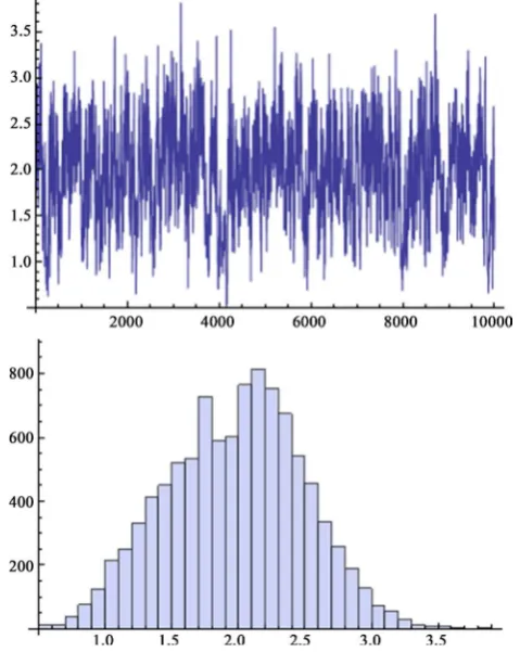
[image:6.595.87.540.657.721.2]

[image:7.595.194.434.82.379.2]

Figure 1.Simulation number of α generated by MCMC method and its histogram.

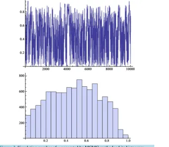
[image:7.595.193.433.405.706.2]

[image:8.595.158.500.86.381.2]

Figure 3.Simulation number of p generated by MCMC methodand its histogram.

Under these data, we compute the approximate MLEs, bootstrap and Bayes estimates of α β, and p using MCMC method results are given in Table 1 and Table 2. Note that Table 2 gives the 95%, approximate MLE confidence intervals, two bootstrap confidence intervals and approximate credible intervals based on the MCMC samples. Figures 1-3 show simulation number of WG parameters generated by MCMC method and the corres-ponding histogram.

References

[1] Green, E.J., Roesh Jr., F.A., Smith, A.F.M. and Strawderman, W.E. (1994) Bayes Estimation for the Three Parameter Weibull Distribution with Tree Diameter Data. Biometrics, 50, 254-269.

[2] Adamidis, K. and Loukas, S. (1998) A Lifetime Distribution with Decreasing Failure Rate. Statistics & Probability Letters, 39, 35-42.

[3] Marshall, A.W. and Olkin, I. (1997) A New Method for Adding a Parameter to a Family of Distributions with Applica-tion to the Exponential and Weibull Families. Biometrika, 84, 641-652. http://dx.doi.org/10.1093/biomet/84.3.641

[4] Adamidis, K., Dimitrakopoulou, T. and Loukas, S. (2005) On a Generalization of the Exponential-Geometric Distribu-tion. Statistics & Probability Letters, 73, 259-269.

[5] Kus, C. (2007) A New Lifetime Distribution. Computational Statistics & Data Analysis, 51, 4497-4509.

http://dx.doi.org/10.1016/j.csda.2006.07.017

[6] Souza, W.A., Morais, A.L. and Cordeiro, G.M. (2010) The Weibull-Geometric Distribution. Journal of Statistical Computation and Simulation, 81, 645-657. http://dx.doi.org/10.1080/00949650903436554

[7] Barreto-Souza, W. (2011) The Weibull-Geometric Distribution. Journal of Statistical Computation and Simulation, 81, 645-657. http://dx.doi.org/10.1080/00949650903436554

[8] Hamedani, G.G. and Ahsanullah, M. (2011) Characterizations of Weibull-Geometric Distribution. Journal of Statistic-al Theory and Applications, 10, 581-590.

[9] Balakrishnan, N. and Sandhu, R.A. (1995) A Simple Simulation Algorithm for Generating Progressively Type-II Cen-sored Samples. The American Statistician, 49, 229-230.

Boston. http://dx.doi.org/10.1007/978-1-4612-1334-5

[11] Gilks, W.R., Richardson, S. and Spiegelhalter, D.J. (1996) Markov Chain Monte Carlo in Practices. Chapman and Hall, London.

[12] Gamerman, D. (1997) Markov Chain Monte Carlo: Stochastic Simulation for Bayesian Inference. Chapman and Hall, London.

[13] Geman, S. and Geman, D. (1984) Stochastic Relaxation, Gibbs Distributions, and the Bayesian Restoration of Images.

IEEE Transactions on Pattern Analysis and Mathematical Intelligence, 6, 721-741.

http://dx.doi.org/10.1109/TPAMI.1984.4767596

[14] Metropolis, N., Rosenbluth, A.W., Rosenbluth, M.N., Teller, A.H. and Teller, E. (1953) Equations of State Calcula-tions by Fast Computing Machines. Journal Chemical Physics, 21, 1087-1091. http://dx.doi.org/10.1063/1.1699114

[15] Hastings, W.K. (1970) Monte Carlo Sampling Methods Using Markov Chains and Their Applications. Biometrika, 57, 97-109. http://dx.doi.org/10.1093/biomet/57.1.97

[16] Gelfand, A.E. and Smith, A.F.M. (1990) Sampling Based Approach to Calculating Marginal Densities. Journal of the American Statistical Association, 85, 398-409. http://dx.doi.org/10.1080/01621459.1990.10476213

[17] Efron, B. and Tibshirani, R.J. (1993) An Introduction to the Bootstrap. Chapman and Hall, New York.

http://dx.doi.org/10.1007/978-1-4899-4541-9