Surmising Consumer Demand System & Structural Changes Using Time Series Data

Munich Personal RePEc Archive

Surmising Consumer Demand System

Structural Changes Using Time Series

Data

Aziz, Babar and Malik, Shahnawaz

BZU Multan

2006

SURMISING CONSUMER DEMAND SYSTEM & STRUCTURAL CHANGES USING TIME SERIES DATA

Professor Dr. Shahnawaz Malik

Chairman Department of Economics, Bahauddin Zakariya University, Multan

Babar Aziz

Ph. D. Scholar / Lecturer in Economics, Government Post Graduate College, Vehari

Wednesday, May 26, 2010

Consumer demand for food and non-food items in Pakistan has attracted the attention

of various researchers. They have employed different parametric approaches, like

single equation, double log models, linear expenditure system and extended linear

expenditure system. Most of the studies were based on household income and

expenditure survey data. Like other household surveys, HIES data do not give

information about prices, due to which price elasticities could not estimated. This

task could not be accomplished partly because, in order to examine the existence and

the nature of structural change and estimation of price elasticities, time series data was

required. In this context the present study is a step ahead. In this analysis time series

data has been used on meat group from 1950-51 to 2003-2004. We estimated the

linear approximation of almost ideal demand system (LA/AIDS). The model is used

to estimate the parameters of meat demand equations. Furthermore, the existence and

the nature of the structural change is checked by using LA/AIDS. The results from

LA/AIDS model show a shift in consumer demand in case of chicken in 1991-92.

Price and expenditure elasticities have also been calculated. The estimates of price

SURMISING CONSUMER DEMAND SYSTEM & STRUCTURAL CHANGES USING TIME SERIES DATA

1. INTRODUCTION

There is hardly an area of economic theory which does not require at least some

knowledge of household consumer behavior. For most of the economic policies the

importance of empirical evidence on consumer behavior seems indisputable. The

close interaction between the theoretical considerations and empirical specification

along with the availability of new types of data and innovating computational

technology have particularly made the analysis of the consumer behavior an

attention-grabbing field of research in recent years.

The analysis of consumer behavior is applicable to a wide range of economic

problems, such as growth and distribution of income, the impact of alternative tax

structures, the implications of rationing and credit constraint, the cost benefit analysis,

the choice of cost of living index, the inter temporal allocation of consumption and

the dynamics of asset accumulation, the determination of real rate of interest and the

economics of uncertainty and information.

The most widely explored area of consumer behavior in empirical literature has been

the estimation of the consumer demand in a static framework. Since the appropriate

panel data are rarely available, most of the empirical studies have been restricted to

the estimation of the Engle curves. Several attempts have been made, however, to

The former empirical research on this subject has been constricted by the limitations

of the available functional forms for the demand models. However, in recent years,

the duality theory has produced a large number of attractive flexible functional forms

which include the Translog System, the Quadratic Expenditure System, the

Generalized Cobb Douglas and Leontief System, the Rotterdam Model and the

Almost Ideal Demand System. During the past ten years or so, a large volume of

empirical literature has also appeared in Pakistan,1 but, most of the researchers used

restrictive functional forms, such as double log and linear expenditure system. The

inherited drawbacks of these functional forms, in detail, are listed in section 2.

Not surprisingly, the evidence on price and income elasticities from the existing

studies on Pakistan is mixed, mainly, due to the variety of methods employed and the

data used. This study shows that during the past two decades food consumption

patterns have changed. This change can partly be explained by movement in relative

prices of food and partly by change in income distribution and poverty.2 However, we

cannot rule out the possibility that some non-price factors, such as changes in tastes,

which may also have been instrumental in bringing about a structural change in

consumer preferences. This phenomenon has received no attention, whatsoever, in

previous consumer demand studies. The fact to the matter is that the existing studies

on Pakistan could not estimate changes in consumer preference because of using cross

sectional data.

1

See, for example, Rehman (1963), Bussink (1970), Khan (1970), Siddique (1982), Malik (1982), Malik and Ahmad (1985), Ali (1985), Malik, Abbas and Ghani (1987), Ahmad and Ludlow (1987), Ahmad, Ludlow and Stern (1988), Alderman (1988), Malik, Mushtaq and Ghani (1988), Burney and Akmal (1991), Burney and Khan (1991) and Burki (1997).

2

The objective of this study is to estimate consumer preferences for meat group using

Pakistan’s annual time series disappearance data from 1950-51 to 2003-2004. The

study tests for the existence of and the nature of the structural change in meat group

by

a) Examining the trends in per capita consumption of meat group,

b) Estimating consumer preferences in the conventional framework of parametric

demand analysis.

On the parametric demand analysis side the linear approximate version of the Almost

Ideal Demand System (LA/AIDS) of Deaton and Muellbauer is used to estimate the

parameters of the food demand equations, price and expenditure elasticities. Most of

the estimated price (own and cross) and income elasticities are significant and

reasonable in magnitude. The inclusion of constants and dummies in LA/AIDS allows

us to gain some insight about the structural change in consumer preferences.

2. STUDIES ON CONSUMER DEMAND IN PAKISTAN

Several empirical studies have been demeanour on consumption patterns in Pakistan.

The studies discussed here are almost exhaustive in the area of consumption analysis.

These studies have addressed different issues relating to household consumption

patterns in rural and urban households. Most of these studies have been published in

late 1980's or early 1990's. For an easy exposition a tabular demonstration is added,

by the end of this section, containing a bird’s eye view on these listed studies. Before

1980s, the field of consumer demand analysis in Pakistan was quiescent. This was

However, the publication of HIES 1979 and availability of computer software’s

generated interest in this area, which has produced several new studies.

The estimation techniques used for price and income elasticities range from simple

double-log or semi-log form to most sophisticated AIDS model. The estimates

obtained by Rehman (1963), Siddiqui (1982), Malik (1982), Malik and Ahmad

(1985), Burney and Khan (1991) have employed the double-log, log linear or

semi-log functional forms. However, it is well known that these forms violate the

integrability condition and thus cannot be deduced by maximizing a utility function.

A cohesive and more serious problem in applied work is that these forms also violate

the Engel aggregation condition. Yoshihara (1969) noted that the criterion of Engel

aggregation may be of a little consequence when only one equation is being

estimated, but in a complete system, violation of this condition gravely affects the

internal consistency of the results. If this condition is imposed on the system all the

income elasticities become equal to one, which is not mesmerizing either.

The other popular approach for consumer demand analysis in Pakistan has been the

LES of Stone (1954) and the ELES of Lulch (1973). For instance, Ali (1985), Ahmad

and Ludlow (1987), Malik, Mushtaq and Ghani (1988), Ahmad, Ludlow and Stern

(1988) and Burney and Khan (1990, 1991) have used the LES and ELES. One

obvious advantage of using LES and ELES is that we can obtain estimates of

subsistence quantities. Nonetheless, the functional form assumed by ELES is quite

restrictive. King (1979, 1981) has pointed out that the property of approximate

proportionality in LES between price and income elasticities does not have any

The LES has another defect that for certain values of prices and income the predicted

expenditures become negative. However, this is clearly not satisfactory from a

theoretical view point [Parks (1969)]. Furthermore, the inferior goods are excluded by

LES. Inferiority can only occur for goods withβ_i <0; but this violates concavity and

if permitted, would result in goods having positive price elasticity. Similarly, if

concavity is to hold, no two goods may be complements; every good must be

substitute for every other good. No one can claim to have "discovered" that goods are

substitutes from the results obtained using LES. Moreover, the effect of relative prices

on saving cannot be measured at all with LES. Since, the total expenditure is

exogenously fixed no matter what happens to relative prices savings remain

unaffected. Additive preferences in the LES imply that the marginal utility of one

good is independent of the quantity of the other goods consumed. This is not a

plausible assumption, especially for food commodities, and therefore, has been found

invalid for even broader commodity groupings [Deaton and Brown (1972)].

More recently, Alderman (1988) has estimated consumer price and income elasticities

by using the AIDS model of Deaton and Muellbauer (1980 a) on Micro data of the

HIES 1979 and published price series of relevant commodities for the four quarterly

rounds in which the Household Survey was conducted. More specifically, Alderman

(1988) employed the linear approximation version of the AIDS model called

LA/AIDS, but used the elasticity formulas of the AIDS, which is not appropriate.

Clarifying on this point Green and Alston (1990) have reported that using AIDS

elasticity formulas in LA/AIDS specification is only appropriate when either the

Burki (1997) has also implemented the LA/AIDS model, and has used the correct

elasticities formulas; suggest by Green and Alston (1990), on time series

disappearance data for nine food commodities. He also tested his data for consistency

with Generalised Axiom of Revealed Preference (GARP). Based on his results, Burki

(1997) identified structural change in the demand for chicken.3

3

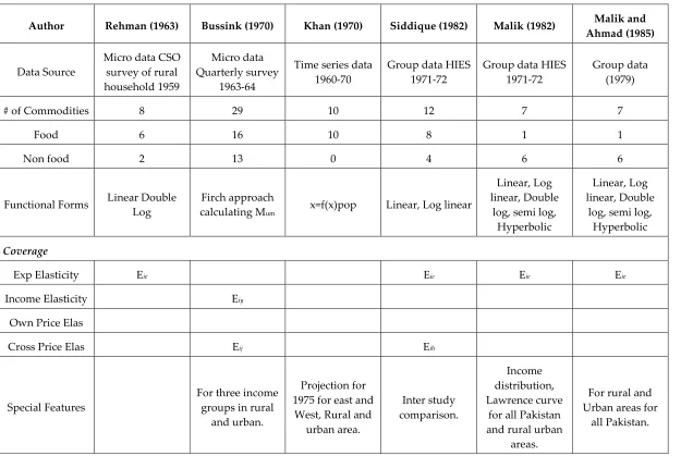
Tabular Representation of Studies on Consumer Demand in Pakistan

Author Rehman (1963) Bussink (1970) Khan (1970) Siddique (1982) Malik (1982) Malik and Ahmad (1985)

Data Source

Micro data CSO survey of rural household 1959

Micro data Quarterly survey

1963-64

Time series data 1960-70

Group data HIES 1971-72

Group data HIES 1971-72

Group data (1979)

# of Commodities 8 29 10 12 7 7

Food 6 16 10 8 1 1

Non food 2 13 0 4 6 6

Functional Forms Linear Double Log

Firch approach

calculating Mum x=f(x)pop Linear, Log linear

Linear, Log linear, Double

log, semi log, Hyperbolic

Linear, Log linear, Double

log, semi log, Hyperbolic

Coverage

Exp Elasticity Eie Eie Eie Eie

Income Elasticity Eiy

Own Price Elas

Cross Price Elas Eij Eih

Special Features

For three income groups in rural

and urban.

Projection for 1975 for east and

West, Rural and urban area. Inter study comparison. Income distribution, Lawrence curve

for all Pakistan and rural urban

areas.

For rural and Urban areas for

all Pakistan.

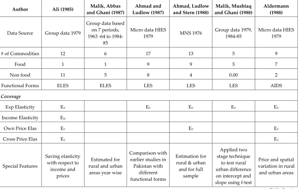
Author Ali (1985) Malik, Abbas and Ghani (1987)

Ahmad and Ludlow (1987)

Ahmad, Ludlow and Stern (1988)

Malik, Mushtaq and Ghani (1988)

Aldermann (1988)

Data Source Group data 1979

Group data based on 7 periods, 1963 -64 to

1984-85

Micro data HIES

1979 MNS 1976

Group data 1979, 1984-85

Micro data HIES 1979

# of Commodities 12 6 17 13 5 9

Food 1 1 9 9 5 7

Non food 11 5 8 4 0.00 2

Functional Forms ELES ELES LES LES LES AIDS

Coverage

Exp Elasticity Eie Eii Eie Eie Eie

Income Elasticity Eiy

Own Price Elas Eii Eii Eii

Cross Price Elas Eij Eij

Special Features

Saving elasticity with respect to

income and prices

Estimated for rural and urban

areas year wise

Comparison with earlier studies in

Pakistan with different functional forms

Estimation for rural & urban and for full

sample

Applied two stage technique

to test rural urban difference on intercept and slope using f-test

Price and spatial variation in rural and urban areas

Author Burney and Khan (1990) Burney and Khan (1991) Burki (1997)

Data Source Micro data HIES 1984-85 Micro data 1984-85 Time series data 1972-93

# of Commodities 6 12 8

Food 0 11 8

Non food 6 1 0.00

Functional Forms ELES LES, Log Linear LA\AIDS

Coverage

Exp Elasticity Eie Eie

Income Elasticity Eiy

Own Price Elas Eii Eii

Cross Price Elas Eij Eij

3. SPECIFICATION OF THE MODEL

Ever since Stone (1954) first estimated a system of demand equation, derived

explicitly from consumer theory, there has been a continuing search for alternative

specifications and functional forms. Many models have been proposed, but perhaps

the most important in current use were the Rotterdam and the Translog models. Both

of the models have been extensively estimated and have, in addition, been used to test

the homogeneity and symmetry restrictions of the demand theory. In 1980, the Almost

Ideal Demand System (AIDS) was proposed by Deaton A. and John Muellbauer

(1980a, 1980b), which has considerable advantages over other models. The AIDS

Model has become the model of choice for many applied demand analysts. It is

relatively easy to account for this popularity. The model is grounded in a

well-structured analytical framework, accommodates certain types of aggregation, satisfies

the axiom of choice exactly, is apparently easy to estimate, and permits testing of the

standard restrictions of the classical demand theory.

Linear approximate version of the AIDS (LA/AIDS) model is employed to estimate

the demand parameters developed by Deaton A. and Jhon Muellbauer (1980a).4

Symbolically, the LA/AIDS model is defined as

ln ln 1, ,

n

t

i i ij jt i t

j t

x

w p i n

p

α γ β   µ

= + +  + =

 

∑

Where pis the price index defined by

0

1

ln ln ln ln 1, ,

2

n n n

t j jt ij it jt

j i j

p =α + α p +   γ p p t = T

 

∑

∑∑

4

and the parameters γ 'sare defined as

* *

1 2

ij ij ji ji

γ =  γ γ+ =γ

 

  (3.3)

Where W_it is the expenditure share of the ith good, p_itis the price and x_tis total

expenditure.

The most interesting feature of the LA/AIDS model, from an econometric point of

view, is that it is close to being linear. Apart from the expression pin (3.1) the

LA/AIDS model can be estimated equation by equation using the OLS. As defined by

equation (3.2),p is a linearly homogenous function of individual prices. In many

practical situations, where prices are relatively collinear, pwill be approximately

proportional to any appropriately defined price index. Such an index can be calculated

directly before estimation so that equation (3.1) becomes straightforward to estimate,

which is in sharp contrast to the estimation of the Translog model [Deaton, A. and

John Muellbaur (1980a and 1980b)].

The theoretical restrictions, i.e, adding up, homogeneity, and symmetry, on equation

(3.1) apply directly to the parameters. Adding up requires that the marginal

propensities to spend on each good sum to unity and that the net effect of a price

change on the budget be zero. The adding up conditions are given by

1 0 0

n n n

i ij i

i i i

α = γ = β =

Whereas the homogeneity and the symmetry are defined, respectively, by

0

n

ij j

γ =

∑

ij ji

γ =γ (3.6)

Provided that restrictions in (3.4), (3.5), and (3.6) hold, equation (3.1) represents a

system of demand functions which add up to total expenditure

(

∑

)

homogeneous of degree zero in prices and total expenditure taken together, and which

satisfy Slutsky symmetry conditions. In the absence of changes in relative prices and

“real” expenditure

( )

point for predictions using the model. Changes in the relative prices work through the

termsγ_ij; each γ_ijrepresents 102times the effect on the ith budget share of a 1 percent

increase in the jth price with

( )

operate through the β_icoefficients; these add to zero and are positive for luxuries and

negative for necessities. However, unrestricted estimation of the AIDS will only

automatically satisfy the adding-up restrictions so that the AIDS once more offers the

opportunity of testing homogeneity and symmetry.

For this linear approximate version of the AIDS model, using elasticity formulas of

the AIDS model be inappropriate [Green and Alston (1990)]. Therefore, we use the

More specifically, in case of n goods we have n2simultaneous equations for

uncompensated elasticities of the form

(

)

ln

ij i

ij ij j k k kj kj

k i i

w w p

w w

γ β

η = − +δ −  + η +δ 



∑

Equation (3.7) can be expressed in matrix notation as

[

] [

]

1

E= BC+I − A+ −I (3.8)

Where the typical elements are a_ij = − +δ_ij

(

) (

)

where δ_ijis known the Kronecker delta

(

)

(

)

in B (an n×1vector); C_j =w_jlnp_j in C (an 1×nvector) and I an identity matrix. The

income elasticities will be measured by N (an n×1 matrix) as

[

]

N = +I BC − B i+ (3.9)

Where N expresses an n-vector of expenditure elasticities, and i is an n unit vector.

Compensated elasticities will be estimated as

*

E= +E NW′ (3.10)

Where E is the matrix of uncompensated price elasticities, N is the matrix of income

4. DATA AND VARIABLES DESCRIPTION

Time series data from 1950-51 to 2003-2004 is used in order to estimate the

parameters of the LA/AIDS model for consumer demand for meat group5 in Pakistan.

Data on personal consumption expenditures was searched out from the Economic

Survey. Per capita consumption of meat was calculated by using the annual

disappearance PCC QP IMP EXP

POP

+ −

 

=

 

 

6

data from Statistical Yearbook of

Pakistan. We have got our hands on the data of population, consumer price index and

implicit price deflator from the Economic Survey. We have acquired price data, which

is an average of twelve centres, from Monthly Statistical Bulletin of the Federal

Bureau of Statistics [Government of Pakistan (various issues)].

5. EMPIRICAL RESULTS

The system of equation for the LA/AIDS model was estimated using iterative Zellner

efficient procedure. Time series data from 1950-51 to 2003-2004 is used for four meat

commodities (meat group) and an equation for other goods. Homogeneity and

symmetry restrictions, in terms of model parameters, are imposed. Since the shares

add up to one, only four out of five equations are independent. Therefore, to ensure

the non singularity of the error co-variance matrix, the equation for others is deleted.

The estimated parameters are invariant to the deleted equation since iterative Zellner

efficient method is followed.7 The parameters of the deleted equation are recovered

using the restrictions for homogeneity and symmetry.

5

Meat group include beef, mutton, chicken and fish. 6

Per capita consumption (PCC) = [Total quantity produced in the economy (QP) in the specific year say 1950-51+ Imports of that year (IMP) - Export of that year (EXP)] / Total population (POP).

7

The time series analysis assumes that the structure of demand and the values of the

co-efficient remain stable over the period under consideration. It is possible that

structure over time may gradually change. The effects of such shift on demand

co-efficient have been recognized [George and King (1971)]. If the change in structure is

clearly identifiable, a shift variable can be introduced in the regression equation. Shift

variable could be introduced in the demand function through dummy variable whose

values are either zero or one, depending upon the period of the observation. Another

way to handle changes in structure is to break the period in to sub periods during

which no change in structure has occurred. One difficulty with this approach is that

the number of observations per sub period may be small for statistical analysis.

Because the exact time for the expected structural change was also not known,

therefore, we varied the breakpoints for one period dummy to investigate structural

change.

Econometric estimates and associated t-values of the parameters in the LA/AIDS

model with homogeneity and symmetry restriction imposed are in Table 5.1. Table

5.1 shows that the intercept terms for beef, mutton and fish are positive and

statistically significant at 10% level of significance except for fish and chicken. This

indicates an exogenous growth in the demand for these commodities, independently

from the movement in prices and income. The exact time for the expected structural

change was not known, therefore, we varied the break time for one period dummy

between 1950-51 to 2003-2004. It is analyzed that the dummy for fish is statistically

significant at 10% level of significance for the period 1991-92. The trend growth for

exogenous growth in the share of fish demand has declined after 1991-92. The

observed decrease in the demand of fish after 1991-92 may be explained by changes

in tastes.

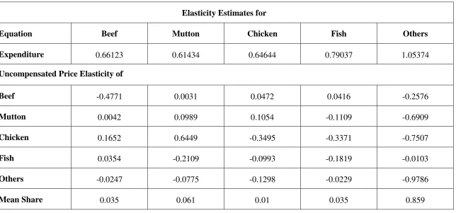
The estimated expenditure elasticities and uncompensated price elasticities are

exhibited in Table 5.2. The expenditure elasticities for all commodities are positive

ranging from a minimum of 0.61434 (for mutton) to 0.79037 (for fish). The

expenditure elasticity for fish is comparatively higher as compared to other meats.

The expenditure elasticities for chicken and beef are 0.64644 and 0.66123

respectively. These results imply that the component of meat group in Pakistan have

the status of necessities. This is expected due to the smaller shares of expenditures on

meat in our sample.

All the uncompensated own price elasticities are negative except for mutton and are

reasonable in magnitudes. The ownprice elasticities vary from 0.1819 (for fish) to

-0.4771 (for beef). While for mutton it is 0.0989. The positive sign for own price

elasticity of mutton may be explained by the violation in curvature condition8 since

only four of the five eigen values were negative and one eigen value was positive. The

cross price substitution effects between beef and mutton, beef and chicken and beef

and fish show that they are substitutes while the cross price effects between mutton

and fish, chicken and fish show their complementary relationship. In other words, we

find that red meats (beef and mutton) are substitutes in nature.

8

Table 5.1 Parameter Estimates of the LA/AIDS Model

Parameter Estimates

Equation Beef Mutton Chicken Fish Others

Constant 0.022

(1.806)* 0.0418 (1.672)* 0.011 (1.299) 0.023 (1.36) -0.098 (-1.864)*

Expenditure -0.012

(-1.042) -0.24 (-1.041) -0.035 (-0.442) -0.072 (-0.475) 0.046 (0.972)

Dummy 0.14

(0.41) -0.017 (-0.242) -0.004 (-0.174) -0.079 (-1.687)* 0.864 (0.6)

Beef 0.177

(2.648)*** -0.006 (-0.063) 0.015 (0.358) 0.0096 (0.172) -0.019 (-1.246)

Mutton -0.006

(-0.063) 0.066 (3.273)*** 0.062 (0.85) -0.078 (-0.732) -0.064 (-1.975)**

Chicken 0.015

(0.358) 0.062 (0.85) 0.065 (1.09) -0.035 (-0.735) -0.011 (-0.941)

Fish 0.0096

(0.172) -0.078 (-0.732) -0.035 (-0.735) 0.028 (2.971)*** -0.018 (-0.909)

Others -0.02

(-1.25) -0.64 (-1.975)** -0.11 (-0.941) -0.018 (-0.909) 0.112 (1.702)*

Note: Figures in parentheses are asymptotic t-values.

Table 5.2Uncompensated Elasticities for the LA/AIDS Model

Elasticity Estimates for

Equation Beef Mutton Chicken Fish Others

Expenditure 0.66123 0.61434 0.64644 0.79037 1.05374

Uncompensated Price Elasticity of

Beef -0.4771 0.0031 0.0472 0.0416 -0.2576

Mutton 0.0042 0.0989 0.1054 -0.1109 -0.6909

Chicken 0.1652 0.6449 -0.3495 -0.3371 -0.7507

Fish 0.0354 -0.2109 -0.0993 -0.1819 -0.0103

Others -0.0247 -0.0775 -0.1298 -0.0229 -0.9786

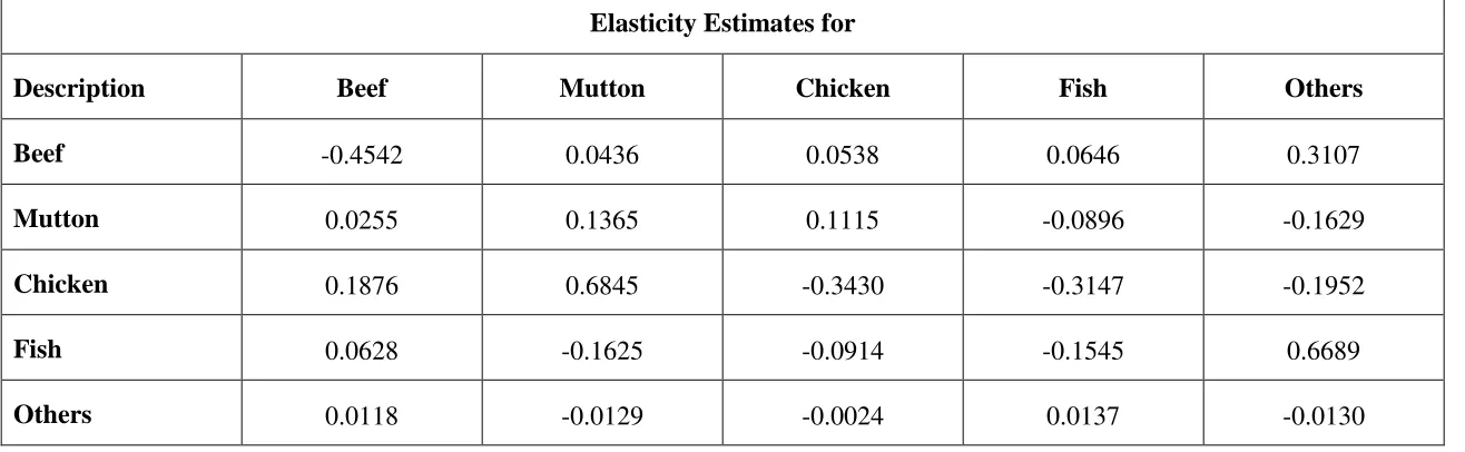
Table 5.3 Compensated Elasticities for the LA/AIDS Model

Elasticity Estimates for

Description Beef Mutton Chicken Fish Others

Beef -0.4542 0.0436 0.0538 0.0646 0.3107

Mutton 0.0255 0.1365 0.1115 -0.0896 -0.1629

Chicken 0.1876 0.6845 -0.3430 -0.3147 -0.1952

Fish 0.0628 -0.1625 -0.0914 -0.1545 0.6689

Comparison of our result with other studies is not easy to make due to different data

sets and estimation techniques used by earlier studies. Most of the studies used double

log forms, linear expenditure system or its extension. Only studies by Alderman

(1988) and Burki (1997) offer results that can be compared with our results, since

they employed LA/AIDS model. The magnitudes of our elasticities are smaller than

Aldermans, which is as expected.

However, a comparison with Burki (1997) and Alderman (1988) is possible because

both have employed LA/AIDS model for their analysis. Alderman has estimated price

elasticities by introducing price variations using for quarterly prices for which four

rounds of survey was completed. However, the problem with Alderman’s estimation

is that it uses incorrect elasticity formulas for the AIDS model. The magnitude of

elasticities from cross sectional data is expected to be smaller than the time series

data. Likewise the magnitude of our elasticities are relatively smaller than

Alderman’s, who used HIES data. On the contrary, the higher magnitude of

Alderman’s elasticities for composite commodities is surprising. Composite

commodities assume that all the included commodities have same income as well as

price elasticities, which is again misleading. The estimates of expenditure or income

elasticities obtained in various studies are arranged in Appendix B1. The cross price

as well as own price are reported in Appendix B2.

6. CONCLUSIONS

This study estimates consumer demand and their responsiveness to prices and income

LA/AIDS model is adopted to estimate consumer preferences. The commodities

included in the meat group beef, mutton, chicken and fish.

The LA/AIDS model was estimated using iterative Zellner efficient procedure with

adding-up, homogeneity and symmetry conditions imposed. Tests of structural change

with the LA/AIDS model do support a shift in demand for fish in 1991-92. More

specifically, the negative and significant dummy for fish suggests that the exogenous

growth in the share of fish demand has declined after 1991-92. The observed decrease

in the demand of fish can be explained by changes in tastes. The estimated own price

elasticities for beef, chicken and fish are negative and reasonable in magnitudes.

However, the sign for mutton’s own price elasticity was positive, which is surprising.

This may be explained by the violation in the negativity condition. The cross-price

substitution effects between beef and mutton shows that these are substitutes while all

other combinations depict complementary relationships. We also find that expenditure

elasticities for all included commodities are positive and less than unity, which means

REFERENCES

Ahmad, E., and S. Ludlow (1987). Aggregate and Regional Demand Response Patterns in Pakistan. Pakistan Development Review. 26(4): 645-657.

Ahmad, E., S. Ludlow and N. Stern (1988). Demand Response in Pakistan: A Modification of the Linear Expenditure System for 1976. Pakistan Development Review. 27(3): 293-308.

Alderman, H. (1988). Estimates of Consumer Price Response in Pakistan using Market Price as Data. Pakistan Development Review. 27(2): 89-107.

Alderman, H. and David E. Salin (1993). Substitution Between Goods and Leisure in a Developing Country. American Journal of Agricultural Economics. 75: 857-883.

Ali, M. Shaukat (1985). Household Consumption and Saving Behaviour in Pakistan. An Application of Extended Linear Expenditure System. Pakistan Development Review. 24(1): 23-38.

Bouis, Hawarch E. (1992). Food Demand Elasticities by Income Group by Urban and Rural Populations for Pakistan. Pakistan Development Review. 31: 997-1017.

Burki, Abid A. (1997). Estimating Consumer Preferences for Food Using Time Series Data of Pakistan. Pakistan Development Review. 36(2): 131-153.

Burndt, Ernst R. (1991), The Practice of Econometrics: Classic and Contemporary. Addision-Wesley, Reading, Massachusetts.

Burney, Nadeem A., and Ashfaque H. Khan (1990). Household Size, its Composition and Consumption Pattern in Pakistan: An Empirical Analysis of Household Level Data. Unpublished Paper.

Burney, Nadeem A., and Ashfaque H. Khan (1991). Household Consumption Patterns in Pakistan An Urban-Rural Comparison using Micro Data. Pakistan Development Review. 30: 145-171.

Bussink, W. C. F., (1970). A Complete Set of Consumption Coefficients for West Pakistan. Pakistan Development Review. 10(2): 193-231.

Deaton, A. and Allan Brown (1972). SURVEYS in Applied Economics. MODELS of Consumer Behaviour. Economic Journal. 82: 1145-1236.

Deaton, A. and John Muellbaur (1980 a). An Almost Ideal Demand System. Economic Review. 70: 312-326.

George, P. S., and G. A. King (1971). Consumer Demand for Food Commodities in the U.S. with Projections for 1980. Giannini Foundation Monograph. 26: 1-77.

Green, R., and Julian M. Alston (1990). Elasticities in AIDS Model. American Journal of Agricultural Economics. 72: 442-445.

Khan, M. I. (1970). Demand for Food in Pakistan in 1975. Pakistan Development Review. 10(3): 310-333.

King, Richard A. (1979). Choices and Consequences. American Journal of Agricultural Economics. 61: 839-848.

King, Richard A. (1981). Choices and Consequences: Reply. American Journal of Agricultural Economics. 63: 176-177.

Lulch, C. (1973). The Extended Linear Expenditure System. European Economic Review. 4: 21-32.

Malik, Shahnawaz (1982). Analysis of Consumption Patterns in Pakistan. Pakistan Economic and Social Review. 20(2): 108-122.

Malik, Shahnawaz and R. Ahmad (1985). Analysis of Household Consumption in Pakistan. Government College Economic Journal. 28(1,2): 97-106.

Malik, S. J., K. Abbas and E. Ghani (1987). Rural-urban Differences and Stability of Consumption Behaviour: An Intertemporal Analysis of the Household Income and Expenditure Survey Data for the Period 1963-64 to 1984-85. Pakistan Development Review. 26(4): 673-684.

Malik, S. J, M. Mushtaq and E. Ghani (1988). Consumption Pattern of Major Food Items in Pakistan: Provincial, Sectoral and Intertemporal Differences 1979 to 1984-85. Pakistan Development Review. 27(4): 751-766.

Parks, R. W. (1969). System of Demand Equations: An Empirical Comparison of Alternative Functional Forms. Econometrica. 37 (Oct.): 629-650.

Rehman, A. (1963). Expenditure Elasticities in Rural West Pakistan. Pakistan Development Review. 3(2): 232-249.

Siddiqui, R. (1982). An Analysis of Consumption Pattern in Pakistan. Pakistan Development Review. 21(4): 275-296.

Stone, R. H. (1954). Linear Expenditure System and the Demand Analysis: An Application to the Pattern of British Demand. Economic Journal. 64: 511 -527.

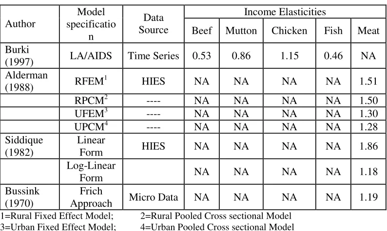
Appendix

Table B1:

Estimates of income elasticities obtained in various studies

Income Elasticities Author Model specificatio n Data

Source Beef Mutton Chicken Fish Meat

Burki

(1997) LA/AIDS Time Series 0.53 0.86 1.15 0.46 NA

Alderman

(1988) RFEM

1

HIES NA NA NA NA 1.51

RPCM2 ---- NA NA NA NA 1.50

UFEM3 ---- NA NA NA NA 1.30

UPCM4 ---- NA NA NA NA 1.28

Siddique (1982)

Linear

Form HIES NA NA NA NA 1.86

Log-Linear

Form NA NA NA NA 1.18

Bussink (1970)

Frich

Approach Micro Data NA NA NA NA 1.19

1=Rural Fixed Effect Model; 2=Rural Pooled Cross sectional Model 3=Urban Fixed Effect Model; 4=Urban Pooled Cross sectional Model

Table B2:

Estimates of own and cross price elasticities obtained in various studies

Cross & Own Price Elasticities of Author Model specificati -on Commo-dities

Beef Mutt

on

Chic

ken Fish

Own Price Elasticity of

Meat only

Burki LA/AIDS Beef -0.58 0.24 0.20 -0.10 NA

Mutton 0.13 -0.29 -0.22 -0.55 NA

Chicken 0.69 -1.37 -0.22 0.37 NA

Fish -0.10 -1.02 0.12 -0.53 NA

Alderman RFEM1 ---- NA NA NA NA -0.29

RPCM2 ---- NA NA NA NA -0.07

UFEM3 ---- NA NA NA NA -1.01

UPCM4 ---- NA NA NA NA -1.06