Implications of University Resource Allocation under Limited Internal Adjustability

http://dx.doi.org/10.4236/tel.2015.55074

How to cite this paper:Abe, Y. and Watanabe, S.P. (2015) Implications of University Resource Allocation under Limited In-ternal Adjustability. Theoretical Economics Letters, 5, 637-646. http://dx.doi.org/10.4236/tel.2015.55074

Implications of University Resource

Allocation under Limited

Internal Adjustability

Yasumi Abe, Satoshi P. Watanabe

Hiroshima University, Higashi-Hiroshima, Japan

Email: [email protected], [email protected]

Received 22 July 2015; accepted 9 October 2015; published 15 October 2015

Copyright © 2015 by authors and Scientific Research Publishing Inc.

This work is licensed under the Creative Commons Attribution International License (CC BY). http://creativecommons.org/licenses/by/4.0/

Abstract

This paper provides a theoretical framework for explaining counterintuitive behaviors of a uni-versity choosing an unfavorable consequence in the long term while attempting to optimally allo-cate its resources in the short term. Our analysis demonstrates the process through which con-flicting interests among different departments within an institution may lead to an internal alloca-tion arrangement, which would not necessarily yield the highest possible outcome for the whole.

Keywords

University Decision Making, Resource Allocation, Prestige Maximization

1. Introduction

Regardless of profit or non-profit nature of productive activities, every organization faces the challenge of achieving objectives through internally allocating limited resources. An institution of higher education, for in-stance, is recognized as a prestige-seeking entity allocating limited resources among academic units, while pro-viding multiple products and services for their stakeholders, which include students, parents, communities, and governments [1]-[9]. Conflicting interests within a higher education institution, however, are documented in James [5] and Massy [6], for different departments competing in a zero-sum game with the faculty trying to in-crease the prestige of only their particular department rather than the overall prestige of the institution. Moreover, Johnson and Turner [10] attribute differences in the number of tenure-track or tenured faculty across academic departments to political forces within the institution, which causes the “stickiness of the adjustment process”.

re-638

sources into multiple activities. The analysis is carried out particularly with not-for-profit organizations such as higher education institutions and hospitals in mind, whose aims are considered to be serving the public need un-der financial constraints, yet seeking to improve social reputation or prestige [11]-[13].

2. Prestige Function and Existence of the Optimal Allocation

Assume that an institution of higher education provides N distinguishable fields of study as well as functionally differentiated outputs such as student teaching, research, community services, or a mixture of these services, from which it gains separately independent prestige p_i for i=1, 2,,N. There exists no definite ceiling for achievable prestige, but it is assumed to be non-negative

(

p

i

≥

0

)

, and let pi be a continuous and strictly

in-creasing function of financial input x_i≥0, which is internally allocated to the ith field of activity. The value of prestige being equal to zero in a specific field i is equivalent to nonexistence of the activity within the institution,

and thus p_i=0 only when x_i =0. Let p_i be also regulated by d

( )

0 0 d

i

i

p

x = ,

d 0 d

i

i

p

x > , and

d

0

d i

i x i

p

x →→∞ ,

for i=1, 2,,N. In other words, the prestige function

p x

_i

( )

_i is depicted as a typical S-shaped curve. The overall prestige of an institution is conceived as the sum of the partial prestige collected from each activity

( )

1 N

i i i

P

=

∑

₌

p x

, and the institution allocates the available resources,

1 N

i i

X

=

∑

₌

x

, so as to maximize its over-all prestige.

The basic setup formulated as above enables us to explore the optimizing allocation arrangement, which maximizes the overall prestige of an institution.1 Considering that the institutional activities are bound by the

resource constraint

1 N

i i

X

=

∑

₌

x

, the optimization problem is simply denoted as

{ } ₁

( )

₁

max subject to ,

i

N N

i i i

x

∑

_i= p x X =

∑

_i=x

with the required first-order condition

( )

d

( )

d

0, , and .

d d

j j

i i

i j

p x

p x

i j i j

x − x = ∀ ≠ (1)

The second-order condition for maximization

( )

2

2 2 1

d

0, d

N

i i i

i i

p x x

x δ

=

≤

∑

(2)

must also be satisfied for an arbitrary vector of

(

δ

x₁,,

δ

xN

)

∈N, where δ indicates an infinitesimal change

and satisfies

∑

N_i=1

δ

x

_i

=

0

. Then, we may state the following proposition.

Proposition 1. For a sufficiently small amount of available resources, a university never finds the optimal al-location set, which yields the highest possible institutional prestige.

Proof: See Appendix.

For intuitive validity of Proposition 1, assume a university with N = 2 and an allocation arrangement

(

x

1

=

X x

,

2

=

0

)

; that is, department 1 receives all the resources while department 2 receives none. Even if a

small amount of the resources

δ

x are transferred from department 1 and reallocated to department 2, i.e.,

(

x

1

= −

X

δ

x x

,

2

=

δ

x

)

, the level of prestige gained by department 2,

p

2

(

x

2

=

δ

x

)

, could be smaller than the

prestige lost by department 1,

p x

₁

(

₁

=

X

)

−

p x

₁

(

₁

= −

X

δ

x

)

, due to the S-shaped partial prestige curves. In such a scenario, the university concentrates all the resources into one department without being able to find the highest potential institutional prestige. The proof of Proposition 1 demonstrates that there exists such a thre-shold, i.e.,

X

<

min

{

x

₁*

,



,

x

_N*

}

, below which the solution to the optimization problem only finds the prestige “minimizing” allocation set.2

1_{Abe and Watanabe [14], based on this framework, demonstrate that enhancement of interdisciplinary effort may hinder prestige} maximiza-tion of a university, through misallocamaximiza-tion of internal resources.

2 * i

x indicates the level of input maximizing the value of d ( )

d i

i i

p x

639

3. Optimal Allocation Set and Attainable University Prestige

In this section, we assume that the total financial resources granted to a university (by the state or other stake-holders) in one period is proportionate with the institutional prestige established in the previous period. The university strives for the highest possible overall prestige, as exemplified in global university rankings, through optimally allocating the available resources as much as the internal “adjustability” permits, which of course is confined by the internal rigidity existing due to conflicting interests among competing departments [5][6][10]. We examine whether the financial resources allocated repeatedly over time under such environments converge to any certain steady point.

3.1. Stable Management Point

Assume that the total budget granted to a university in period t+1 is determined according to the assessment of reputation or prestige demonstrated in the previous period t. The total funding received by the university in period t+1 is then represented by X( )t+1 = X P

( )

( )t , where P( )t indicates the overall institutional prestige

measured in period t. Additional assumptions are imposed on the total resources that

X

( )

0

=

0

, d

( )

0 d X P

P > ,

( )

2

2

d

0 d

X P

P < , and it is bounded above, thus approaching the least upper bound as P→ ∞ which simply

indi-cates that the amount of resources awarded to a university has a limit.

Suppose now that a university begins its operations at t=0 with the original allocation arrangement

( ) ( ) ( )

{

0 0 0

}

1 , 2 , , n

x x  x and X( )0 =

∑

_iN₌₁x_i( )0 .3 Given the initial resources and allocation, the university earns the

to-tal prestige P( )0 in period t=0, and the budget granted for the next period is determined as X( )1 =X P

( )

( )0 . We assume that the preliminary arrangement

{ }

xi( )1 in period t=1 is made at the beginning of that period,

based on the allocation rule applied to each department i, ( )

( ) ( ) ( )

1

1 0

0

i i

X

x x

X

= . The final arrangement

{ }

xi( )1 in

pe-riod t=1 is then made upon modifying the preliminary set in search of even higher attainable prestige than would otherwise be achieved with

{ }

x_i( )1 .4 The adjustment made from the preliminary allocations

{ }

x_i( )1 to

the final arrangement

{ }

x_i( )1 is denoted by

δ

x_i( )1 =x_i( )1 −x_i( )1 for all i=1,,N.

In practice, however, there might be internal rigidity in altering the allocation ratio assigned to each depart-ment, which makes it difficult for an institution to change the allocation composites drastically from the pre-viously assigned ratios, as noted by Johnson and Turner [10] as “stickiness of the adjustment process”. There-fore, the modifications in the allocation arrangement may be realized only within a limited range of magnitude.

In order to accommodate such internal rigidity, the adjustment made from the initial allocation set

{ }

xi( )1 to the

final arrangement

{ }

x_i( )1 may be restrained by the following inequalities:

( ) ( )

( ) ( ) ( )

1 1 1

1 1

1

for some constant 0,

N _i

i _i

x P P

C C

x P

δ

=

−

< >

∑

(3)

3_{For notational simplification in this and following sections, we write}

{ }

( )t i

x to denote

{

1( ), ( )2, , ( )

}

t t t

n

x x x .

4_{Thus, we assume that the preliminary arrangement is made in each period at first, based on the subjective criterion} ( ) ( ) ( ) ( )

1 1

t

t t

i t i

X

x x

X

+ + ₌

. The

shift in the allocations made from the initial set

{ }

( )1

i

x to the final arrangement

{ }

( )1

i

640 ( )

( )

1

1 1

for some constant 0,

N _i

i _i

x

L L

x

δ

=

< >

∑

(4)

where ( )1

( )

( )1

1 N

i i i

P =

∑

₌ p x is the overall prestige achievable with the preliminary allocations

{ }

x_i( )1 , and

( )1

( )

( )1 1 N

i i i

P =

∑

₌ p x is the final overall prestige realized in period t=1. The summations in the conditions (3)

and (4) are defined for all the departments for which the resource allocated in the previous period was not equal to 0. The inequality in (3) means that a large modification in the allocations does not occur unless a large in-crease in the total prestige can be expected as a result of the modified arrangement. The inequality in (4) simply describes the condition whereby even if a large increment would be obtained in the total prestige, the modifica-tion of the arrangement is limited by a certain ceiling. Both C and L are unique to each university and regu- late the organizational adjustability to internally shift the allocations from the initial

{ }

x_i( )t to the final set

( )

{ }

t i

x in a single period. Under these conditions, we are now ready to state the following proposition regarding the convergence of the process.

Proposition 2. Given any initial conditions, a university reaches the optimal allocation arrangement at which the maximal prestige is achieved: 1) with all N departments, or 2) with only N−m departments, where m represents the number of department closures, or otherwise 3) no resources are allocated to any of the N de-partments (i.e., the university ceases operations).

Proof: See Appendix.

What is stated in Proposition 2 appears a sterile result at first, but an important implication drawn from

Proposition 2 is that the point of convergence may represent an inferior state for a university in terms of achieving the highest potential objective. In the following subsection, it is demonstrated for a heuristic example with N=2, that a university may end up with optimizing at a “corner solution” where the institutional prestige realized as a result of “optimal” choices over time is lower than that yielded at the other corner solution.

3.2. An Example of Non-traditional Corner Solution

Suppose that a sufficiently funded university with N=2 departments is originally optimizing in the interior at

0

t= . If the university resources plunge into a threshold, such as

X

<

min

{

x x

₁*

,

₂*

}

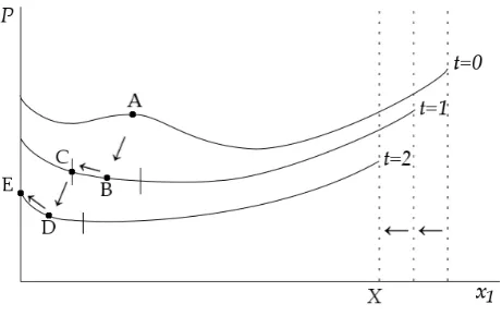
, in period t=1 due to a severe budget cut, then the optimizing position shifts from the local maximum (point A) to the global minimum (point B) as depicted in Figure 1. The internal rigidity in settling financial matters, due to conflicting interests among competing departments, limits its mobility to shift the allocations within a certain capacity. Thus, the university moves toward a new allocation set, which yields the highest prestige, but it does so only within a li-mited range (indicated with “tick marks” in Figure 1 below).

[image:4.595.199.430.562.707.2]

Then, whether the new allocation set moves to the right or left from the prestige minimizing point B depends on the highest overall prestige found “within the mobility range”. In the graph, the new allocation set is reached

641

at point C, where the level of gained institutional prestige is the highest within the “ticked range”. If the institu-tional budget in period t+1 is determined by the overall prestige realized in the previous period t, then the resources granted in period t=2 would be even smaller than the resources received in period t=1. Beginning from point D in period t=2, the highest institutional prestige within the mobility range is found at point E, where all the resources are concentrated into department 2, while department 1 is left with no funding, i.e., an allocation set

(

x

₁

=

0,

x

₂

=

X

)

.

As described so far, the process would typically repeat over the courses of modified allocations and corres-ponding overall prestige, ultimately reach the leftmost “corner solution” where the total budget X is poured into only one of the two departments. As verified in this example, a university may well end up with an unde-sirable outcome in the long run even though the short-run optimizing process is achieved repeatedly. The result is dependent on the location of the initial allocation, internal adjustability which regulates the mobility range, as well as the shape of the total prestige curve in the neighborhood of new allocations.

4. Conclusion

This paper examines an important scenario, which a standalone institution of higher education is predicted to follow in order to achieve its potential maximal performance when the available resources are severely limited. Our result clearly indicates that a collection of multiple departmental performances does not necessarily yield the highest level of institutional prestige; that is, diversification of functional specialties is not necessarily the prudent approach to attaining the highest potential recognition when a university faces a scarcity in its financial resources. We also find that the limited internal adjustability caused by conflicting interests within a university impedes the goal of attaining the best outcome in the long term although the university “optimally” allocates its resources in the short term.

Acknowledgements

This paper was completed while S.P.W. was a visiting scholar at the University of California, Berkeley. We are grateful to colleagues at UC Berkeley for valuable comments and discussions on earlier drafts of the paper and would like to express sincere gratitude for all the encouragement and general resources provided by the Center for Studies in Higher Education and UC Berkeley.

References

[1] Baumol, W.J., Panzar, J.C. and Willig, R.D. (1982) Contestable Markets and the Theory of Industry Structure. Mar-court Brace Jovanovich, New York.

[2] Breneman, D.W. (1976) The Ph.D. Production Process. In: Froomkin, J.T., Jamison, D.T. and Radner, R., Eds., Educa-tion as an Industry, National Bureau of Economic Research, Cambridge, 1-52.

[3] Cohn, E., Rhine, S.L.W. and Santos, M.C. (1989) Institutions of Higher Education as Multiproduct Firms: Economies of Scale and Scope. The Review of Economics and Statistics, 71, 284-290. http://dx.doi.org/10.2307/1926974

[4] Del Rey, E. (2001) Teaching versus Research: A Model of State University Competition. Journal of Urban Economics, 49, 356-373. http://dx.doi.org/10.1006/juec.2000.2193

[5] James, E. (1990) Decision Process and Priorities in Higher Education. In: Hoenack, S.A. and Collins, E.L., Eds., The Economics of American Universities: Management, Operations, and Fiscal Environment, State University of New York Press, Buffalo, 77-106.

[6] Massy, W.F. (1996) Productivity Issues in Higher Education. In: Massy, W.F., Ed., Resource Allocation in Higher Education, University of Michigan Press, Ann Arbor, 49-86.

[7] Melguizo, T. and Strober, M.H. (2007) Faculty Salaries and the Maximization of Prestige. Research in Higher Educa-tion, 48, 633-668. http://dx.doi.org/10.1007/s11162-006-9045-0

[8] Brewer, D.J., Gates, S.M. and Goldman, C.A. (2001) In Pursuit of Prestige: Strategy and Competition in U.S. Higher Education. Rutgers Transaction Publishers, Piscataway.

[9] Cyrenne, P. and Grant, H. (2009) University Decision Making and Prestige: An Empirical Study. Economics of Educa-tion Review, 28, 237-248. http://dx.doi.org/10.1016/j.econedurev.2008.06.001

642

[11] Frank, R.G. and Salkever, D.S. (1991) The Supply of Charity Services by Nonprofit Hospitals: Motives and Market Structure. RAND Journal of Economics, 22, 430-445. http://dx.doi.org/10.2307/2601057

[12] Horwitz, J.R. and Nichols, A. (2009) Hospital Ownership and Medical Services: Market Mix, Spillover Effects, and Nonprofit Objectives. Journal of Health Economics, 28, 924-937. http://dx.doi.org/10.1016/j.jhealeco.2009.06.008

[13] Newhouse, J. (1970) Towards a Theory of Nonprofit Institutions: An Economic Model of a Hospital. American Eco-nomic Review, 60, 64-74.

643

Appendix

Proof of Proposition 1

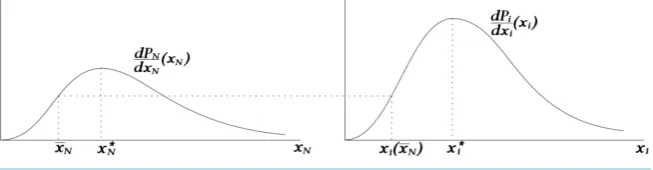
For all the N fields of activities, place the corresponding values of partial prestige

(

p x₁

( )

₁ ,,p_N

( )

x_N

)

in decreasing order of d

( )

*

d i i i p x

x for i=1, 2,,N , where

* i

x

indicates the level of input maximizing the

val-ue of d

( )

d i i i p x

x . That is,

( )

( )

* 1 *

1 1 d d d d i i i i i i p p x x x x + + +

≥ so that the last element in the order, d

( )

*

d N N N p x

x , gives the

low-est value of all.

Suppose the resource allocated to the Nth field is

x

_N

≤

x

*_N . Since, by the proposed construct,

( )

*

( )

* d d d d N i N i N i p p x x

x ≤ x for 1≤ ≤ −i N 1 , there exists an allocation for every i=1,,N−1 such that

( )

( )

d d d d N i N i N i p p x x

x = x , which lies to the left of

( )

* d *

, d i i i i p x x x    

[image:7.595.85.538.125.366.2] [image:7.595.152.479.623.708.2]

 . Denote such an allocation as

x x

i

( )

N as shown in Figure S1below.

More explicitly,

( )

(

( )

)

d d , d d N i

N i N

N i

p p

x x x

x = x (A1)

and the individually allocated resources sum to

X x

( )

_N

=

∑

_iN₌₁−1

x x

_i

( )

_N

+

x

_N.

It is obvious that

x x

_i

( )

_N is continuous and strictly increasing over the domain

0

≤

x

N

≤

x

N*, and

x

i

( )

0

=

0

.

For the allocation arrangement

(

x x

₁

( )

_N

,



,

x

_N−1

( )

x

_N

,

x

_N

)

with the budgetary constraint

X

=

X x

( )

_N , the

first-order condition (1) is satisfied by construct for all i and

j i

(

≠

j

)

, and the positive definite condition (2) for minimization is also satisfied. Thus, for a sufficiently small amount of available resources, i.e.,

( )

( )

*

N N

X

=

X x

<

X x

where

x

_N

<

x

_N* , there exists an allocation arrangement

(

x x

₁

( )

_N

,



,

x

_N−1

( )

x

_N

,

x

_N

)

which minimizes the prestige of an institution.

For the uniqueness of the (global) minimum in the interior, suppose the total resources available for the insti-tution is reduced further to an extremity such that

X

<

min

{

x

₁*

,



,

x

*_N

}

. Under such an extreme condition,

however the resource is allocated, every coordinate ,d

( )

d i i i i p x x x    

  must lie on the left side of

( )

* d *

, d i i i i p x x x      .

For if this is not the case and even a single allocation ,d

( )

d i i i i p x x x    

  lies on the right side of

( )

* d *

, d i i i i p x x x    

 , it

implies

x

_i

≥

x

_i* which by itself exceeds the total available resources X. In order to simplify the notation in

the following discussion, we denote

x

_i

=

x x

_i

( )

_N .

644

Suppose there exists, other than

(

x

₁

,



,

x

N

)

, a different allocation set

(

x



1

,



,

x



N

)

which yields the

extre-mum under the same resource constraint. Since these allocations must satisfy

∑

_iN₌₁

x



_i

=

∑

N_i=1

x

_i

=

X

, there exist

for i≠ j at least one i such that x_i >x_i and at least one j such that x_j <x_j. If this is not the case, then it implies that the two allocation sets are identical, which contradicts the initial statement for the two sets being

differentiated from each other. Since both ,d

( )

d i i i i p x x x    

   and

( )

d , d i i i i p x x x    

  lie on the left side of

( )

* d *

, d i i i i p x x x    

  while

( )

d , d j j j j p x x x      

   and

( )

d , d j j j j p x x x      

  also lying on the left side of

( )

* d *

, d j j j j p x x x      

 , the

following relation must be established for individual allocations x_i, x_i, x_j, and x_j,

( )

( )

d

( )

d

( )

d d

.

d d d d

j j

i i

i i j j

i i j j

p p

p p

x x x x

x  > x = x > x  (A2)

The result in (A2) clearly indicates d

( )

d

( )

d d j i i j i j p p x x

x  ≠ x  , contradicting the required first-order condition (1), and so there exists no allocation set other than

(

x

₁

,



,

x

_N

)

which yields the extremum under the budgetary

constraint

X

=

X x

( )

_i . This proves that for sufficiently small

X

<

min

{

x

₁*

,



,

x

*_N

}

, the allocation set

(

x

1

,



,

x

N

)

is the only arrangement capable of reaching the extremum, which turns out to be the global

mini-mum found in the interior.

Suppose further that optimization is sought with the closures of m departments. Then, the financial re-sources initially allotted to these departments would be redistributed among the existing N−m departments with the same budgetary constraint

X

=

∑

N_i=1

x

_i

=

∑

_iN m₌₁−

x

_i. As a result of the closures of the m fields,

how-ever, the relation

min

{

x

₁*

,



,

x

*_N

}

≤

min

{

x

₁*

,



,

x

*_{N m−}

}

is established, from which we find that the binding con-dition

X

<

min

{

x

₁*

,



,

x

*_{N m−}

}

continues to be sustained for an operation of the N−m activities. Therefore, the preceding result is preserved for the resource level X<min

{

x₁*,,x_{N m}*₋

}

, yielding the minimum as the only extremum in the interior. _

Proof of Proposition 2

Let

{ }

xi( )0 be the allocation arrangement made at the outset with the constraint

( )0 ( )0 1 N

i i

X =

∑

₌ x . The partial

prestige is defined by pi( )0 = p xi

( )

i( )0 for i=1,,N , which sums to the overall institutional prestige

( )0 ( )0 1 N

i i

P

=

∑

₌

p

. Then, the total resources received by the institution in period t=1 may be denoted as

( )1

( )

( )0

X =X P , based on which the new allocation arrangement is made. The initial and subjective allocation criterion at the beginning of a new period is transmitted from the immediately previous period

( ) ( ) ( ) ( ) 1 1 t t t

i _t i

X

x x

X − −

= for all i, and modifications are made to the initial set

{ }

xi( )1 in search of even higher

pres-tige within the limited range of the organizational adjustability, reaching the final allocation set

{ }

x( )_i1 . This process may be applied iteratively for arbitrary large t periods. Then, there exist only two possible scenarios to be considered.

Scenario 1. X( )0 ≤X( )1

Since x_i( )0 ≤x_i( )1 for all i=1,,N, the preliminary total prestige P( )1 evoked at the beginning of period

1

t= is at least as large as the total prestige realized in the previous period; that is,

( )

( )1 ( )0

1 N

i i i= p x ≥P

Be-645

cause the modified allocation

{ }

x( )_i1 is made with additional adjustments to the preliminary set

{ }

x_i( )1 in

search of even higher overall prestige, it is obvious that ( )0

( )

(1) ( )1

1 N

i i i

P ≤

∑

₌ p x =P which in turn connects to

the budget to be received in the next period, X( )1 ≤X( )2 . A simple iteration of this process demonstrates that the total resources reveal a non-decreasing sequence, i.e., X( )0 ≤X( )1 ≤≤X( )t ≤, for t periods.

The equality X( )t−1 =X( )t for all t≥2 periods in the above sequence is established only when

( )t 2 ( )t1

P − =P − , which means that the preliminary allocation set

{ }

x_i( )t−1 has in fact reached the (local)

maxi-mum and equals the previous allocation set

{ }

x( )it 2 −

. Since the initial allocation ratios are determined by the

subjectively fixed criterion ( )

( ) ( ) ( )

1

1 2

2

t

t t

i _t i

X

x x

X −

− −

−

= , the result gives X( )t−1 = X( )t−2 . Thus, the equality

( )t 1 ( )t

X − =X holds only for the set

{ }

x_i( )0 giving the (local) maximum with X( )0 =X( )1, which is equivalent to the convergence of the sequence at the outset. Therefore, in the first scenario of a non-decreasing sequence, only the strictly increasing sequence of total resources, X( )0 < X( )1 <<X( )t <, remains to be examined.

Scenario 2. X( )0 > X( )1

If the total resources granted in period t=2 increase, X( )1 <X( )2 , as a result of the allocation arrangement in period t=1, then the sequence X( )t begins to strictly increase afterwards. This is equivalent to the first scenario with a strictly increasing sequence. If the equality X( )1 =X( )2 holds, the preliminary allocation in

pe-riod t=2 is given by x_i( )2 =x_i( )1 for all i because of the subjectively assigned criterion ( )

( ) ( ) ( )

2

2 1

1

i i

X

x x

X

= . Since the preliminary prestige in period t=2 is the same as the total prestige realized in period t=1, i.e.,

( )2

( )

( )2

( )

( )1 ( )1

1 1

N N

i i i i

i i

P =

∑

₌ p x =

∑

₌ p x =P , the relation P( )2 ≥P( )1 must hold after the modifications are made

from the preliminary set

{ }

xi( )2 to the final arrangement

( )

{ }

2

i

x . The equality between the prestige in two

pe-riods, P( )2 =P( )1 , is established only if the modifications would produce no increment in the total prestige, which implies that the set

{ }

x_i( )2 has in fact yielded a (local) maximum and no further reallocation would be

sought thereafter. In this case, the total resources become X( )2 = X( )3 ==X( )t =, for t≥2, which clearly indicates the convergence of the sequence. If the total prestige is strictly increasing, P( )2 >P( )1 , then the total resources also increase strictly, X( )3 >X( )2 , and the sequence X( )t begins to reveal a strictly increasing pat-tern as in the first scenario. Finally, if X( )1 >X( )2 , then the relation between X( )2 and X( )3 must be ex-amined through the same process described above.

To summarize both scenarios, other than the clearly convergent cases, the total resources X( )t evolve in one of the following paths:

• Strictly increasing

• Strictly decreasing up to a certain point, then strictly increasing thereafter

• Strictly decreasing

The common feature for all three paths is that they eventually turn to monotone sequences (either strictly in-creasing or dein-creasing). Since the sequence

X P

( )

is bounded below

(

X P

( )

≥

0

)

and has the least upper

bound, the sequence X( )t is convergent either way.5 If X( )t is strictly increasing, then it approaches a con-stant limit, whereas if X( )t is strictly decreasing the sequence converges either to 0 or a non-zero limit. If

5_{This is simply the result of the Monotone Convergence (Sequence) Theorem, which states that every bounded monotone sequence in }

646

( )t

X converges to 0, it clearly means that every allocation in

{ }

x_i( )t converges to 0. Therefore, it suffices to

only examine the cases where X( )t is a monotone sequence and convergent to a non-zero limit.

We first note that convergence of X( )t means the convergence of P( )t because the total resource X( )t is a continuous function of the total prestige,

X P

( )

. We now examine how the resources and allocations progress over time. The overall change in the allocation arrangement from period t−1 to period t is decomposed into two separate movements from the set

{ }

x_i( )t−1 to

{ }

x_i( )t and from

{ }

x_i( )t to the final arrangement

{ }

x( )_it . Let

( )

{ }

t

i

x

δ

and

{ }

δ

x_i( )t represent such modifications made at each stage,

( )t ( )t ( )t 1

i i i

x x x

δ

_{= −} −

(A3)

( )t ( )t ( )t

i i i

x x x

δ

= − _(A4)

with corresponding changes in the total prestige

( )

( )

( ) ( )1 1

N

t t t

i i i

P p x P −

=

∆ =

∑

− (A5)

( ) ( )

( )

( )

1

.

N

t t t

i i i

P P p x

=

∆ = −

∑

(A6)

Substituting the definition ( )

( ) ( )1 ( )1

t

t t

i t i

X

x x

X − −

= in equation (A3) yields

( ) ( )

( ) ( ) ( )

( ) ( ) ( ) ( )

1

1 1 1

1 1 .

t t t

t t t t

i t i i t i

X X X

x x x x

X X

δ − − − −

− −

−

= − = (A7)

Therefore, the convergence of sequence X( )t results in convergence of

δ

x_i( )t to 0 in the above relation

(A7), which in turn implies that

( )

( )t

( )

( )t 1

i i i i

p x −p x − , thus its summation ∆P( )t in (A5), also converge to 0. Furthermore, a combined definition of (A5) and (A6) yields P( )t −P( )t−1 = ∆P( )t + ∆P( )t . The finding that ∆P( )t

converges to 0, along with the convergent sequence P( )t , implies ∆P( )t converges to 0. Since we are examin-ing the cases where the sequence X( )t converges to a non-zero limit, the allocation x_i( )t is not equal to 0 for all i. Then, the denominator of the right-hand side in (A8) below, which is simply a rewritten form of the rigid-ity condition (3) for period t,

( )

( )

( )

( )

( )

1

1

,

t t

N _i

t N t

i _{i i i}

i

x P

C

x p x

δ

= ₌

∆ <

∑

∑

(A8)

has a positive sign, which affirms that the right-hand side of the inequality in (A8) converges to 0. This means that

δ

x_i( )t on the left-hand side also converges to 0, and so we have shown that both

δ

x_i( )t and

δ

x_i( )t

con-verge to 0. Finally, using the relation x_i( )t −x_i( )t−1 =

δ

x_i( )t +

δ

x_i( )t which is drawn from the definitions (A3) and

(A4), we have proved that x_i( )t converges.

If the point of convergence does not yield any of 1), 2), and 3) stated in Proposition 2, the value of prestige added by the modification process from

{ }

x_i( )t to

{ }

x_i( )t is arbitrarily large near x_i( )t , which contradicts the fact that both

δ

x_i( )t and

δ

x_i( )t converge to 0. Therefore, the allocation set

{ }

( )t

i

x approaches one of 1), 2), and