Enhancement of Performance Measures using EMD in Noise Reduction Application

(1)

Enhancement of Performance Measures using EMD in

Noise Reduction Application

Kusma Kumari Cheepurupalli

Dept. of Electronics & Communication Engg, Andhra University, Visakhapatnam, A P, India.

Raja Rajeswari Konduri

Dept. of Electronics & Communication Engg, Andhra University, Visakhapatnam, A P, India.

ABSTRACT

Empirical Mode Decomposition (EMD) has been used effectively in the analysis of non-linear and non-stationary signals. As an application in Robust Signal Processing, in this paper we used this method to reduce noise from a corrupted signal which is obtained from a disaster environment. Conventional adaptive algorithms exhibit poor performance if we consider the signal from a real environment. In this paper it has been described how EMD can be applied for noise reduction by breaking the signal down into its components and how it can help in removing the noisy components from the original signal.

Keywords

Adaptive algorithms, LMS, RLS, EMD, Sifting process, Monotonic property, merit measures.

1. INTRODUCTION

Adaptive filters are the digital filters with the coefficients that can change over time. The general idea is to assess how well the existing coefficients are performing and then adapt the coefficient values to improve performance. This approach is useful in two somewhat different application categories. The first category involves filtering requirements that are stationary but unknown. In this case an adaptive filter can be initialized with a guess and then allowed to converge to a better solution. The second category involves filtering requirements that may be loosely bounded in some way, but which vary over time. In the first category, speed of convergence often is a secondary consideration behind the steady-state error remaining in the converged filter. In the second category, steady-state error is important, but the adaptation speed must be sufficient to allow the filter coefficients to track the time-varying requirements. The trade between convergence speed and steady- state error is a fundamental issue in adaptive signal processing. [1]

Empirical Mode Decomposition (EMD) has been proposed recently [2] as an adaptive time-frequency data analysis method. It has been proven to be quite versatile in a broad range of applications for extracting signals from data generated in noisy nonlinear and non-stationary process. In this paper EMD is used to reduce the effect of standard white noise corrupting the signal.

2. ADAPTIVE ALGORITHMS

Adaptive filters have been widely used in communication systems, control systems and various other systems in which the statistical characteristics of the signals to be filtered are either unknown a prior or, in some cases, are slowly

time-variant (non-stationary). Numerous applications of adaptive filters have been described in the literature. Two algorithms popularly used in adaptive filtering are described in the following sections.

2.1 LMS Algorithm

The Least Mean Square (or) LMS algorithm, first introduced in 1960 by Widrow & Hoff [3] is the most widely used of all the adaptive filtering algorithms that have been developed. This algorithm is relatively simple to implement and it provides good performance in a wide range of applications. The LMS algorithm can be described from the Eqn (1) derived by considering the steepest descent algorithm by neglecting some parameters as in [1]:

x(k)

)

k

(

2 w(k)

1)

w(k









(1)

where x is the input sample vector, w is the tap weight and k is iteration count, ε is a small positive constant and μ is the convergence factor that determines the step size. If μ is too large the convergence speed is fast but filtering is not proper. If μ is too small the filter gives a slow response. Since μ is limited for the purposes of stability, the convergence of LMS can be treated as very slow.

2.2 RLS Algorithm

Performance provided by the RLS algorithm is usually superior relative to the LMS algorithm, at a moderate increase in computational complexity. The description of RLS algorithm is given by the below Eqns. (2-3)

(k)u

1)

-w(k

w(k)







* (2)

1)

-P(k

)

k

(

u x

-1)

-P(k

P(k)



H (3)

where P[k] is an N×N matrix, x is an input sample vector, w is tap weight, k is the iteration count and ε is a small positive constant.[1]

(2)

3. EMD AS A FILTERING TECHNIQUE

The EMD adaptively decomposes the input signal into a series of Intrinsic Mode Functions (IMF’s) through the sifting process which is described as follows [4]:

1. Identifies all extrema of input signal x(t) (noise corrupted signal is to be considered here)

2. Generates the upper envelope u(t) and the lower envelope l(t) of extrema and calculate the mean envelope as

2 l(t))

(u(t)

m(t)





3. Subtract m(t) from x(t) to generate the detail

m(t)

x(t)

d(t)



4. Updates x(t) using d(t) and then repeats the steps from 1 to 4 until d(t) satisfies stopping criterion.

The detail is referred to the first IMF as imf1(t). In order to decompose x(t) into a series of IMFs. The above process is repeated as follows:

5. Subtract imf1(t) from x(t) to generate the residual

(t)

imf

-x(t)

)

t

(

r

₁



₁

6. Treats the residual r1(t) as the input signal and repeats the above sifting process to generate the next IMF inf2(t) and residual r2(t)

7. Repeat the step 5 and 6 to generate a series of IMF’s and the last residual rn(t) until the stopping criterion (i.e rn(t) should be monotonic) is satisfied.

(t)

imf

-(t)

r

)

t

(

r

(t)

imf

-x(t)

)

t

(

r

n i -n n 1 1

















The stopping criterion for the EMD process is that the signal which is being decomposed, if its exhibits the monotonic property the decomposition process stops and no further IMFs are produced. Finally the input signal can be represented as the summation of the IMFs as shown in the Eqn (4):









n 1 i n 1

(

t

)

r

(

t

)

imf

x(t)

(4)

where ‘ i ’ is the IMF order. It can be seen that the basic IMF function is adaptively generated from the input signal and there is no parameter that need to be initialized.

4. OBSERVATIONS AND ANALYSIS

In this paper the noise reduction application is implemented for the signal considered in [5] are same considered as the original input signal i.e sin((0.5*pi)*t) with t = 0: 0.1: 15 and the noise signal as standard white noise with zero mean unit variance. In order to give a quantitative evaluation of the trend extraction effect the performance measures such as Root Mean-Square Error (RMSE), Normalized Absolute Error

(ENAE), Signal to Noise ratio (SNR) and Average Systematic Bias (Ebias) of the signal after de-noising are considered [6]: RMSE is given by Eqn (5) as:



 











N 1 t 2

)

t

(

x

-x(t)

N

1 RM SE

(5)

where

x(t)

stands for the original signal and

x

(

t

)



is the de-noised signal. N denotes the length of the signal. The lower the value of the RMSE shows the better noise reduction. It denotes that the estimated signal is more similar to the original signal. The Normalized absolute error (ENAE), normalizes average absolute error of the de-noised signal to average of original signal, and if the value of ENAE is smaller, then error in the de-noised signal is less. ENAE shown in Eqn (6) is expressed as:



  





_N 1 t N 1 t NAE

x(t)

)

t

(

x

E

(6)

Signal-to-noise ratio (SNR) is a traditional evaluation index for the effect of the de-noised signal. The higher value of SNR the better the results. SNR is given by Eqn (7) as:

























   N 1 t 2 N 1 t 2

)

t

(

x

-x(t)

)

t

(

x

log

10 SNR

(7)

Average Systematic Bias (Ebias) reflects the bias of the de-noised signal. A lower value Ebias shows a smaller systematic bias and Ebias can be expressed in Eqn (8) as:



 









_



N 1 t

bias

x

(

t

)

x(t)

N

1 E

(8)

The noise reduction has been performed using the LMS, RLS and EMD.

4.1 Simulation based on LMS algorithm

The adaptive filter design and simulation based on the LMS algorithm is done for the above signal which is corrupted with the standard white noise. The filter order selected in [5] is 2 with a step factor 0.1. Hence in this paper for comparison purpose the same filter orders are considered. In the present paper, the AR (1) coefficients considered here are a1= 0.8 and a2= -0.6 referring the literature [7]. By executing the algorithm using all the above parameters results the use of the LMS in noise reduction. Fig. 1 shows the simulation results. It contains the noise corrupted signal and the filtered output after passing through the LMS adaptive filter.

(3)

RLS in simulation. Fig. 2 shows the learning curve which is plotted by considering error versus number of iterations.

0 5 10 15

-5 0 5

time

A

m

p

li

t

u

d

e

Noise corrupted signal

0 5 10 15

-5 0 5

time

A

m

p

li

t

u

d

e

[image:3.595.328.532.81.338.2]

Output signal from LMS adaptive noise canceller of order 2

Fig. 1 Noise corrupted signal (upper row), filtered output (lower row)

0 50 100 150

0 2 4 6 8 10 12 14 16 18 20

Number of iterations

E

rr

o

r

[image:3.595.68.271.114.398.2]

Learning curve of LMS algorithm

Fig. 2 Learning curve of LMS

4.2 Simulation based on RLS algorithm

The adaptive filter design and simulation based on the RLS algorithm is done for the above signal which is corrupted with the standard noise. The selected filter order is 16 with a lambda and delta [5] as 1 along with AR (1) coefficients a1= 0.8 and a2= -0.6 from the literature [7]. By executing the algorithm using all the above parameters results the use of the RLS in noise reduction. Fig. 3 shows the simulation results which contains the noise corrupted signal and the filtered output after passing through the RLS adaptive filter. As the used filter order is 16, noise reduction is somewhat better in comparison to that of the LMS.

0 5 10 15

-5 0 5

time

A

m

p

li

t

u

d

e

0 5 10 15

-5 0 5

time

A

m

p

li

t

u

d

e

Output signal from RLS adaptive noise canceller of order 16

F ig. 3 Noise corrupted signal (upper row), filtered output

(lower row)

0 50 100 150 0

2 4 6 8 10 12 14 16 18 20

E

rr

o

r

[image:3.595.336.518.381.575.2]

Learning curve of RLS algorithm

Fig. 4 Learning curve of RLS

[image:3.595.68.263.425.616.2]

(4)

With the use of some factorization algorithms these problems can be reduced-[8].

4.3 Simulation based on EMD algorithm

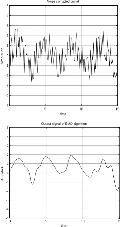
The design and simulation of the EMD is done for the same noise corrupted signal [5] which is considered for the above two algorithms. The simplicity of this algorithm is that there is no need to specify the input parameters like filter order, step factor, lambda, delta, etc. The only requirement to be satisfied is the necessity of input signal considered for decomposition has to obey the ‘non-monotonic property’. Hence this method is popularly used in the analysis of linear and non-stationary applications. As the above input signal satisfies the non-monotonic property the EMD has reduced the noise up to a maximum extent. Fig. 5 shows the simulation results which contains the noise corrupted signal and the output signal after passing through the EMD. The shape of the output signal is slightly disturbed because of the influence of the noise signal at earlier stages of IMF calculation. Fig. 6 shows the learning curve which is plotted as error versus number of iterations. From the learning curve of the EMD we can observe that the magnitude of the error is less in comparison with adaptive algorithms. For plotting the learning curve the error considered here is the summation of all IMF’s.

0 5 10 15 -5

-4 -3 -2 -1 0 1 2 3 4 5

time

A

m

p

li

tu

d

e

0 5 10 15

-5 -4 -3 -2 -1 0 1 2 3 4 5

time

A

m

p

li

tu

d

e

[image:4.595.329.532.75.240.2]

Output signal of EMD algorithm

Fig. 5 Noise corrupted signal (upper row), EMD output (lower row)

0 50 100 150

0 2 4 6 8 10 12 14 16 18 20

E

rr

o

r

[image:4.595.69.271.332.710.2]

Learning curve of EMD algorithm

Fig. 6 Learning curve of EMD

Tab. 1 shows the calculated parameters using Eqns (5-8) for the three algorithms used in the noise reduction application. From Tab.1 we can observe greater reduction of the RMSE in the EMD. The SNR value obtained for the LMS and the RLS is negative, but it is positive for the EMD. The ENAE and Ebias are obtained somewhat well for the RLS due to the filter order considered [5] is 16. The RLS also exhibits poor performance if the filter order considered is less. From Tab.1 we can observe the performance measures of the RLS if the filter order was taken as 2 (like for the LMS).

Algorithm RMSE ENAE SNR EBias

LMS (Filter order 2)

1.4269 29.9204 -6.0983 0.0880

RLS (Filter order 2)

1.2163 25.2539 -4.7114 0.1239

RLS (Filter order 16)

0.7754 10.8783 -0.8004 0.2065

EMD 0.6765 15.3132 0.3839 0.4952

Table 1: Calculated values of performance measures

The basic issues in any adaptive implementation are speed, complexity and stability. The LMS algorithm is slow and simple and the RLS algorithm is fast and complex. But as per stability requirements both LSM and RLS exhibits stable performance [9]. Among the three algorithms, the EMD shows better performance in noise reduction application. EMD also exhibits stable performance along with moderate speed and less complexity. Hence this method is popularly used for the non-linear and non-stationary signal analysis. The simulation work carried out in this paper can be considered as offline work. This EMD can also be efficiently used for online signal processing applications [10].

5. CONCLUSIONS

[image:4.595.315.536.360.533.2]

(5)

filtering techniques used here. It has been shown that in non-stationary noise environments and low-SNR conditions, the proposed algorithm used here provides the enhancement of the performance levels like describing by SNR, RMSE, etc.

It is obvious that this EMD technique has a great potential. It is not only limited to the domain of signal enhancement but also it does not possess any filter order like LMS and RLS. The principles may be applied and integrated to a wide range of solutions. It also presents exciting possibilities for 2-D signals. However, the EMD is a promising new addition to existing tool-boxes for non-stationary and non-linear signal processing. But it still needs to be better understood. The results reported here are believed to provide a new insight on the EMD and its use, but they are merely of an experimental nature and they clearly call for further studies devoted to more theoretical approaches.

6. ACKNOWLEDGEMENTS

This work is being supported under the project “Robust Signal Processing Techniques for RADAR/SONAR Communications using VLSI Tools” by Ministry of Science & Technology, Department of Science & Technology (DST), New Delhi, India, under Women Scientist Scheme (A) with the Grant No: 100/ (IFD)/8893/2010-11).

7. REFERENCES

[1] C. Britton Rorabaugh, "DSP Primer" Edition, Mc Graw Hill Education publication, 2005.

[2] N.E. Huang, Z. Shen, S.R. Long, M.L. Wu, H.H. Shih, Q. Zheng, N.C. Yen, C.C. Tung and H.H. Liu, “The empirical mode decomposition and Hilbert spectrum for

non-linear and non-stationary time series analysis,” Proc.Roy.Soc London A, Vol.454, pp.903–995, 1998.

[3] Widrow, B. and M.E.Hoff Tr. “Adaptive Switching Circuits,” IRE WESCON, Rec., pt.4, pp 96-104, 1960.

[5] Ying He, Hong He, Li Li, Yi Wu, Hongyan Pan, “The Applications and Simulation of Adaptive Filter in Noise Cancelling”, International Conference on Computer Science and Software Engineering, 2008.

[6] Liu Xin-xia, Han Fu-lian, Wang Jin-gui “Wavelet Extended EMD Noise Reduction Model for Signal Trend Extraction”, Handan Technology Bureau Project, 2009.

[7] Monson Hayes H. “Statistical Digital Signal Processing and Modelling” John Wiley & Sons Inc, Kundli, 2002.

[8] Emmanuel C.Ifeachor et.al “Digital Signal Processing A practical approach” Pearson Education, 2003.

[9] V.UdayShankar, “Modern Digital Signal Processing” PHI, Second Edition, April 2012.