http://dx.doi.org/10.4236/ijaa.2015.53017
Flat Space Cosmology as a Mathematical
Model of Quantum Gravity or
Quantum Cosmology
Eugene Terry Tatum1, U. V. S. Seshavatharam2, S. Lakshminarayana3 1760 Campbell Ln. Ste. 106 #161, Bowling Green, KY, USA
2Honorary Faculty, I-SERVE, Hyderabad, India
3Department of Nuclear Physics, Andhra University, Visakhapatnam, India Email: [email protected], [email protected], [email protected]
Received 25 June 2015; accepted 24 August 2015; published 27 August 2015
Copyright © 2015 by authors and Scientific Research Publishing Inc.
This work is licensed under the Creative Commons Attribution International License (CC BY).
http://creativecommons.org/licenses/by/4.0/
Abstract
We review here the recent success in modeling our expanding universe according to the rules of flat space cosmology. Given only a few basic and reasonable assumptions and a single tional input, our model derives a variety of results which correlate with astronomical observa-tions, including best estimates of the size, total mass, temperature, age and expansion rate of our observable universe. Considering the apparent success of our model, we attempt to explain why we think it works so well, including the fact that it incorporates elements of both general relativity and quantum mechanics. We offer this approach as a possible avenue towards understanding cosmology at the quantum level (“quantum gravity”).
Keywords
Flat space Cosmology, Hubble Parameter, Hubble Radius, CMBR Redshift, Schwarzschild Formula, Hawking Black Hole Temperature Formula, Quantum Gravity
1. Introduction
paper [2], we derived current Hubble radius R0, Hubble time HT (universal age), total mass M0, cosmic temperature T0 and CMBR redshift, knowing only the current Hubble parameter H0 value of 68.6 km/sec/Mpc (2015 Planck survey upper limit). In this paper, we summarize the key mathematical relationships and attempt to explain why such a simple model works so well.
2. Our Key Model Assumptions
Our key model assumptions can be expressed as follows, for any scale from the Planck scale to the scale of our observable universe:
1) Cosmic radius R and total mass MR follow the Schwarzschild formula R 2GM2 R
c
≅ at all times.
2) The cosmic event horizon always translates at speed of light c with respect to its geometric center. Thus, in our model, the Hubble parameter HRcan be expressed as c/R. And considering assumptions 1 and 2 together, the
cosmic Hubble radius can be expressed as 2 2 R R
GM c
R
H c
≅ ≅ and Hubble time (universal age) can be expressed
as R c≅1HR for any stage of cosmic expansion.
3) The possible range of cosmic linear velocity of rotation at the Planck scale can be assumed to be anywhere from zero up to the special relativity limit of c. If we start by assuming the maximum possible value (c), then
3 2
pl c Rpl c GMpl Hpl
ω ≅ ≅ ≅ , where ωpl is the Planck scale angular velocity, Mpl is the Planck mass, Hpl is
the Planck scale Hubble parameter and Rpl, according to assumption 1, is the Planck radius and equals twice the
Planck length. As such, 2.176507949 10 kg8
pl
M ≅ c G≅ × − , and Rpl 2G c G c2 3.23240045 1035m
−
≅ ≅ × ,
and the Planck scale Hubble parameter
(
)
(
3 2)
9.274607607 10 sec42 1pl pl pl
H ≅ c R ≅ c G c G ≅ × − ≅ω in
rad·sec−1.
4) Following thermodynamics of Hawking’s black hole temperature formula [4], at any radius R cosmic temperature T is inversely proportional to the geometric mean of cosmic total mass MR and the Planck mass
pl
M .
3
8π
B R
R pl
c k T
G M M
≅ (1)
3. Our Model Formulae Based on These Assumptions
3.1. Relations between Cosmic Radius, Total Mass and Hubble Parameter
2 2 3
2 2 2
R
R R
Rc c c c
M
G G H GH
≅ ≅ ≅
(2)
2 2
3
2 3 3 4π
3 8π 8π
R R
H c
M R
G GR
≅ ≅
(3)
where R, MR and HR represent cosmic radius, total mass and Hubble parameter, respectively. Average
mass density equaling Friedmann’s critical density is seen in the second line. Hence, our cosmic model is con-stantly “flat” by the Friedmann formula.
3.2. Relations between Temperature, Mass, Radius and Hubble Parameter (Thermodynamics)
3
4π
8π 4π
R pl B R
R pl pl
H H
c c
k T
G M M RR
≅ ≅ ≅ (4)
2
2 1 27 2
1.0272646 10 m K 4π
R
pl B
c RT
R k
≅ ≅ × ⋅
2 2 2
4π 4π
R
pl
R pl B B
T c
H R k ω k
≅ ≅ (6) 2
19 2 1
2
4π 1
2.918356766 10 K sec
R B pl R H k H T − − − ≅ ≅ × ⋅
(7)
where TRrepresents the cosmic temperature for a given cosmic radius R.
4. Our Derivations of Current Cosmological Parameters
Using only our basic assumptions and the equations they generate above, derivations of current values for our observable universe are as follows:
Relations between universal current radius R0, current temperature T0, current Hubble parameter H0, current total mass M0, and current average mass density:
2
2 2 2
0
0 26
1 1 1 1
4π 4π 2.72548
1.3829177 10 m
pl B pl B
c c
R
R k T R k
≅ ≅ ≅ × (8)
(
)
2 2 2 2 0 0 18 14π 4π
1 1
2.72548
2.167826 10 sec 66.89 km sec Mpc
B B pl pl k k H T H H − − ≅ ≅ ≅ × ≅
(9)
2 3
52 0
0
0
9.311752 10 kg.
2 2
R c c
M
G GH
≅ ≅ ≅ × (10)
( )
( )
2 02 27 30 0 2
0 3 3
8.4053137 10 kg m 8π 8π average critical H c G GR
ρ ≅ ρ ≅ ≅ ≅ × − ⋅ −
(11)
where
( )
ρ0 average is the average mass density and( )
ρ0 critical is Friedmann’s critical average mass density. The above-derived radius and mass values simulate a current observable universe with a radius of 14.6 billion light-years and roughly 2 × 10²² visible stars plus 5 × dark matter, roughly 1053 kg.Derived current cosmological values are consistent with 2015 Planck survey data. As per the 2015 Planck survey data, the current value of the Hubble parameter H0 is reported to be:
(
)
(
)
(
)
Planck low : 67.31 0.96 km sec Mpc
Planck low : 67.73 0.92 km sec Mpc
Planck , , low : 67.7 0.66 km sec Mpc
TT P
TE P
TT TE EE P
+ ± + ± + ±
As per the 2015 Planck data, the current value of CMBR temperature T0 is reported to be:
(
)
(
)
Planck low BAO : 2.722 0.027 K
Planck ; ; low BAO : 2.718 0.021 K
TT P
TT TE EE P
+ + ±
+ + ±
As per COBE/FIRAS, CMBR temperature T0 is reported to be:
(
2.7255 0.0006 K±)
.From our recent analysis of conservation of angular momentum in flat space cosmology (pending publication), the maximum possible Planck scale angular momentum is:
(
2)
(
2)
(
)
234 2 1
2
2.10912261 10 kg m sec 2
pl pl pl pl pl pl pl pl
A M R ω M R c R GM c
where
8
1
35
8
2.176507949 10 3.23240045 10
2.99
kg,
7924
m,
and 58 10 m sec
pl pl
M R
c
− −
−
≅ ×
×
≅ ×
≅
⋅
Assuming angular momentum conservation, maximum possible current angular momentum is:
(
2)
0 0 0 0 2
A ≅ M R ω ≤ (13)
Hence, the maximum possible current angular velocity is:
139 1
0
0 2 2
0 0 0 0
2
1.2 10 rad sec
A
M R M R
ω ≤ ≤ ≤ × − ⋅ −
(14)
Based upon this extremely small derived maximum theoretical value, our pending angular momentum paper concludes “this number is well beyond our ability to observe cosmic rotation effects in the present” or, presum-ably, even at the universal age at recombination.
Thus, our model predicts that rotational effects are unlikely to be detectable in higher resolutions of the cos-mic cos-microwave background radiation (CMBR).
As our cosmic model is always assumed to be expanding at light speed, from the beginning of the Planck scale, cosmic age can be expressed as follows:
(
R Rpl)
tc
−
≅ (15)
For the current case, since
( )
Rpl is very small and(
R0−Rpl)
≅R00 0
0 1
R t
c H
≅ ≅ (16)
5. Our Model Correlations with Observed Cosmic Redshifts
We have proposed simple model equations (relations 17 - 23) for observed and predicted cosmic redshifts [2], including the CMBR redshift. One particularly simple model equation under current study is:
0 0
2
3
0 0 0
2
1 1
where and 2 .
x x
x
R GM
Z
R c R
R R M c GH
≅ − ≅ −
< ≅
(17)
and where R0 and Rx represent current and past cosmic radii, respectively. With reference to the assumed
equivalent cosmic temperature [2], redshift term Z can be obtained in the following way:
0
0 0 0
exp 1 ln 1 ln 1
exp ln ln 1 exp ln 1 1
x pl pl
x
pl pl x x
R R
Z
R R
R R R R
R R R R
≅ + − + −
≅ − − ≅ − ≅ −
(18)
From relation (5) it is clear that the cosmic radius is inversely proportional to the squared cosmic temperature. The above relation (17) can be expressed, approximately, as follows:
2 0
0 2
0
1 x 1 where
x x
R T
Z T T
R T
≅ − ≅ − > (19)
2
0 2
0 0
1 where
x x
x
T T
Z T T
T T
≅ − ≅ (20)
This can be compared with the famous relation familiar to modern cosmologists:
0 1 Tt
Z T
+ ≅ (21)
Given our stated basic assumptions, our expanding cosmic model shows average mass-energy density to be inversely proportional to R2. See relation (11). In a very real sense, the deeper an observer from Earth looks into space (and time), the greater the temperature stage and average mass energy density stage of the cosmos one is observing. Thus, each progressively higher temperature stage and average mass density stage of the cosmos is associated with higher gravitational field strengths. So, there must be associated gravitational time dilation ef-fects. This conclusion is firmly grounded in general relativity. Thus, it appears likely that at least a portion of the progressively higher redshift we observe with increasing look-back distance is a manifestation of gravita-tional time dilation. In addition, because of this inverse square relationship over very long distances, plots of proximal galactic redshifts per unit of distance observed would be expected to look relatively linear (as seen by the weaker telescopes of the 1920’s and 1930’s) and deep space galactic redshifts per unit of distance observed would be expected to clearly fall away from linearity, along with decreasing luminosity (as redshifts extend into the infrared range), similar to the 1998 Type Ia supernovae observations [5]. Such an effect may possibly create an illusion of dark energy where there is none. This is for further study.
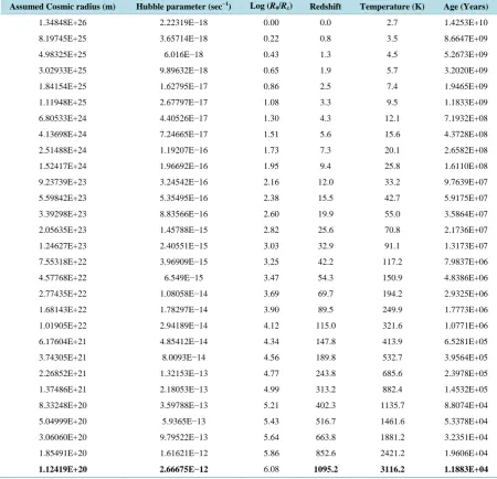
The following graph (Figure 1), according to above relation (17), shows expected cosmic redshift as a func-tion of the log ratio of current cosmic radius (R0) to past cosmic radius (Rx) pertaining to a particular
astronomi-cal observation. In this manner, increasingly greater redshifts would be expected to correspond with more distant galactic observations. However, notice the apparent near-linearity below the radius ratio of about 20 (Log 1.3), and the increasingly nonlinear appearance with deeper space observations. The authors propose that something like this mathematical relationship could be useful in modeling the results of progressively deeper space obser-vations. For data, see Table 1. The last row of Table 1 correlates cosmic radius (Rx), Log (Rx/R0), redshift and universal age corresponding to a temperature of 3116 K.
Thus, simple model formula relations (17) and (20) closely approximate the recombination temperature of
3000K and CMBR redshift of 1093 believed to be related to formation of the first hydrogen atoms.
Of course, since we are modeling flat space cosmology, we are also testing a slightly more complex model formula, Minkowski’s relativistic Doppler formula for flat space:
( )
( )
1 1
1
v c Z
v c +
+ ≅ −
(22)
In order to keep scaling similar to Figure 1, the velocity term v in the Minkowski formula can be substi-tuted with 1−
(
Rx R0)
c where Rx<R0. The reduced relation can be expressed as:(
)
(
0)
02
1x
x
R R Z
R R
−
≅ − (23)
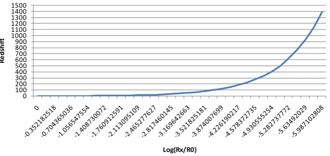
Figure 2shows the Minkowski relativistic Doppler redshift term Z as a function of decreasing log cosmic
radius ratio
(
R Rx 0)
pertaining to progressively deeper space observations. The reader should note that the CMBR redshift of 1093 correlates with the place on the horizontal axis corresponding to log value −5.777. Per-haps more importantly, however, the reader’s attention is directed to the place on the horizontal axis corres-ponding to the log value of −1.5. A greatly magnified portion of this region of Figure 2 would show the nonli-nearity corresponding to the earliest visible galaxies, which appear to be receding at up to about 0.95 c.0 100 200 300 400 500 600 700 800 900 1000 1100 1200
0.
00
0.
22
0.
43
0.
65
0.
86
1.
08
1.
30
1.
51
1.
73
1.
95
2.
16
2.
38
2.
60
2.
82
3.
03
3.
25
3.
47
3.
69
3.
90
4.
12
4.
34
4.
56
4.
77
4.
99
5.
21
5.
43
5.
64
5.
86
6.
08
Re
ds
hi
ft
[image:6.595.95.530.84.244.2]Log(R0/Rx)
Figure 1. Cosmic Redshift vs Log Ratio of Current and Past Cosmic Radii.
Table 1. Cosmic Physical Parameters Obtained with above relations.
Assumed Cosmic radius (m) Hubble parameter (sec−1) Log (R0/Rx) Redshift Temperature (K) Age (Years)
1.34848E+26 2.22319E−18 0.00 0.0 2.7 1.4253E+10
8.19745E+25 3.65714E−18 0.22 0.8 3.5 8.6647E+09
4.98325E+25 6.016E−18 0.43 1.3 4.5 5.2673E+09
3.02933E+25 9.89632E−18 0.65 1.9 5.7 3.2020E+09
1.84154E+25 1.62795E−17 0.86 2.5 7.4 1.9465E+09
1.11948E+25 2.67797E−17 1.08 3.3 9.5 1.1833E+09
6.80533E+24 4.40526E−17 1.30 4.3 12.1 7.1932E+08
4.13698E+24 7.24665E−17 1.51 5.6 15.6 4.3728E+08
2.51488E+24 1.19207E−16 1.73 7.3 20.1 2.6582E+08
1.52417E+24 1.96692E−16 1.95 9.4 25.8 1.6110E+08
9.23739E+23 3.24542E−16 2.16 12.0 33.2 9.7639E+07
5.59842E+23 5.35495E−16 2.38 15.5 42.7 5.9175E+07
3.39298E+23 8.83566E−16 2.60 19.9 55.0 3.5864E+07
2.05635E+23 1.45788E−15 2.82 25.6 70.8 2.1736E+07
1.24627E+23 2.40551E−15 3.03 32.9 91.1 1.3173E+07
7.55318E+22 3.96909E−15 3.25 42.2 117.2 7.9837E+06
4.57768E+22 6.549E−15 3.47 54.3 150.9 4.8386E+06
2.77435E+22 1.08058E−14 3.69 69.7 194.2 2.9325E+06
1.68143E+22 1.78297E−14 3.90 89.5 249.9 1.7773E+06
1.01905E+22 2.94189E−14 4.12 115.0 321.6 1.0771E+06
6.17604E+21 4.85412E−14 4.34 147.8 413.9 6.5281E+05
3.74305E+21 8.0093E−14 4.56 189.8 532.7 3.9564E+05
2.26852E+21 1.32153E−13 4.77 243.8 685.6 2.3978E+05
1.37486E+21 2.18053E−13 4.99 313.2 882.4 1.4532E+05
8.33248E+20 3.59788E−13 5.21 402.3 1135.7 8.8074E+04
5.04999E+20 5.9365E−13 5.43 516.7 1461.6 5.3378E+04
3.06060E+20 9.79522E−13 5.64 663.8 1881.2 3.2351E+04
1.85491E+20 1.61621E−12 5.86 852.6 2421.2 1.9606E+04
[image:6.595.86.537.289.723.2]0 100 200 300 400 500 600 700 800 900 1000 1100 1200 1300 1400 1500
Re
ds
hi
ft
[image:7.595.147.484.84.243.2]Log(Rx/R0)
Figure 2. Redshift vs Decreasing Log (Rx/R0).
not at all conclusive in this regard. Please see 2015 references [6] and [7]. In particular, a very strong case has been made by Jun-Jie Wei, et al., that the Type Ia supernovae data are a better fit for a cosmic horizon coasting along at speed of light c [7]!
This important question requires further study.
6. Summary Discussion
Given the apparent simplicity of our mathematical model, we have been pleasantly surprised by the excellent correlation between derivations from our model formulae and astronomical observations. However, upon closer inspection, the reason for this should be fairly obvious. Science progresses not by completely discarding reliable mathematical models from the past, but by refining them along with improvements in observation. Frequently, the older formulae exist as remnants within the newer refined formulae. Such will ultimately be the case when elements of general relativity and quantum mechanics come together as “quantum gravity”.
In this tradition, our mathematical model incorporates a formula (Schwarzschild) derived from general rela-tivity, combining it with Hubble’s velocity-distance relation [8], conservation of angular momentum (to set a
2 limit on cosmic rotation), and incorporating all of these relationships into formulae (relations 4) which closely resemble Hawking’s black hole temperature formula [4]. Seeds in the development of these mathemati-cal inter-relationships can be followed in references [9]-[14]. It is, therefore, not particularly unreasonable that our mathematical formulation has some relevance to our observable universe. While it may seem mysterious to some observers that quantum terms from the Planck scale, Boltzmann’s constant, and 2 are creeping into our cosmological equations and derivations, we predict that further iterations of this process will ultimately lead us towards a more complete theory of “quantum gravity”.
Acknowledgements
The authors express their thanks to Dr. Abhas Mitra for his kind and valuable suggestions in developing this subject. One of the authors, Seshavatharam U.V.S., is indebted to professors K.V. Krishna Murthy, Chairman, Institute of Scientific Research in Vedas (I-SERVE), Hyderabad, India and Shri K.V.R.S. Murthy, former scien-tist IICT (CSIR), Govt. of India, Director, Research and Development, I-SERVE, for their valuable guidance and great support in developing this subject. Author Dr. E. Terry Tatum would also like to thank Dr. Rudy Schild, Harvard Center for Astrophysics, for his support and encouragement in developing this subject.
References
[1] Tatum, E.T., Seshavatharam, U.V.S. and Lakshminarayana, S. (2015) The Basics of Flat Space Cosmology. Interna-tional Journal of Astronomy and Astrophysics, 5, 116-124. http://dx.doi.org/10.4236/ijaa.2015.52015
[2] Tatum, E.T., Seshavatharam, U.V.S. and Lakshminarayana, S. (2015) Thermal Radiation Redshift in Flat Space Cos-mology. Journal of Applied Physical Science International, 4, 18-26.
[4] Hawking, S.W. (1975) Particle Creation by Black Holes. Communications in Mathematical Physics, 43, 199-220.
http://dx.doi.org/10.1007/BF02345020
[5] Riess, A.G., Filippenko, A.V., Challis, P., et al. (1998) Observational Evidence from Supernovae for an Accelerating Universe and a Cosmological Constant. Astrophysical Journal, 116, 1009-1038. http://dx.doi.org/10.1086/300499
[6] Nielsen. J.T., et al. (2015) Marginal Evidence for Cosmic Acceleration from Type Ia Supernovae. arXiv:1506.01354v2. [7] Wei, J.-J., Wu, X.-F., Melia, F., et al. (2015) A Comparative Analysis of the Supernova Legacy Survey Sample with
ΛCDM and the Rh = ct Universe. The Astronomical Journal, 149, 102. http://dx.doi.org/10.1088/0004-6256/149/3/102
[8] Hubble, E.P. (1929) A Relation between Distance and Radial Velocity among Extra-galactic Nebulae. PNAS, 15, 168- 173. http://dx.doi.org/10.1073/pnas.15.3.168
[9] Seshavatharam, U.V.S. and Lakshminarayana, S. (2015) Primordial Hot Evolving Black Holes and the Evolved Pri-mordial Cold Black Hole Universe. Frontiers of Astronomy, Astrophysics and Cosmology, 1, 16-23.
[10] Seshavatharam, U.V.S. and Lakshminarayana, S. (2014) Friedmann Cosmology: Reconsideration and New Results.
International Journal of Astronomy, Astrophysics and Space Science, 1, 16-26. [11] Pathria, R.K. (1972) The Universe as a Black Hole. Nature, 240, 298-299.
http://dx.doi.org/10.1038/240298a0
[12] Tatum, E.T. Could Our Universe Have Features of a Giant Black Hole? Journal of Cosmology, 25, 13061-13080. [13] Tatum, E.T. (2015) How a Black Hole Universe Theory Might Resolve Some Cosmological Conundrums. Journal of
Cosmology, 25, 13081-13111.
[14] Melia, F. and Maier, R.S. (2013) Cosmic Chronometers in the Rh = ct Universe. Monthly Notices of the Royal