Spurious Instrumental Variables

(1)

Munich Personal RePEc Archive

Spurious Instrumental Variables

Ventosa-Santaulària, Daniel

Escuela de Economía, Universidad de Guanajuato

2007

Online at

https://mpra.ub.uni-muenchen.de/58779/

(2)

Spurious Instrumental Variables

Daniel Ventosa-Santaul`

aria

∗

Abstract

Spurious regression phenomenon has been recognized for a wide range of Data Gene-rating Processes: driftless unit roots, unit roots with drift, long memory, trend and broken-trend stationarity, etc. The usual framework is Ordinary Least Squares. We show that the spurious phenomenon also occurs in Instrumental Variables estimation when using non-stationary variables, whether the non-stationarity component is sto-chastic or deterministic. Finite sample evidence supports the asymptotic results.

Keywords: IV Estimator, Spurious Regression, Broken-Trend stationarity, Unit Root.

JEL Classification: C12, C13, C22.

1 Introduction

Spurious regression—that is, a statistically significant relationship between two independent

random variables—has been uncovered for different forms of non-stationarity in a simple

Least Squares (hereinafter, LS) framework. Indeed, related literature has studied the cases

where the variables are generated as driftless random walks (Phillips 1986), random walks

with drift (Entorf 1997),I(d) processes withdbeing an integer (Marmol 1995), long memory

and fractional integrated processes (Marmol 1998), Trend Stationary (T S) processes,1_as_{T S}

processes with breaks, and, mixed nonstationary DGP’s.2 _{The approach taken in the study}

of spurious regression tends to involve the computation of the asymptotics using increasingly

complex Data Generating Processes (DGP’s), whilst estimation methodology remains the

same (LS). This dependence on LS estimators may be considered somewhat limiting, given

∗_{Corresponding Author: Escuela de Economia, Universidad de Guanajuato. Address: UCEA-Campus}

Marfil Fracc. I, El Establo, Guanajuato Gto 36250 Mexico. e-mail: [email protected]

1

See Hasseler (2000)and Kim, Lee, and Newbold (2004).

2

(3)

the variety of estimators commonly used in applied research—Instrumental Variables (IV)

and Generalized Method of Moments (GMM), for example. To the best of our knowledge,

little consideration has been given to the possibility of a connection between the spurious

phenomenon and the IV estimator.3 _{This paper focuses in the IV regression estimates under}

independent nonstationary variables. We prove that, when there is no relationship between

the regressand, the regressor and the instrument,4_{IV estimates are statistically significant,}

that is, IV regression is spurious. We derive the asymptotic behavior of t-statistics in

IV-estimated regressions, where the DGP consists of two independent and nonstationary

processes with a trending mechanism, be it deterministic with (a possible) structural break

or stochastic. Additionally, some Monte Carlo evidence is presented to account for the

spurious regression phenomenon in finite samples.

2 IV Estimates using Nonstationary Variables

IV is a classical technique in econometrics; it originated as a proposal to solve the

identifi-cation problem in the estimation of demand and supply curves (Wright 1928).5 _Typically,

in text books, IV is proposed as a solution to the problem of omitted variables and, broadly

speaking, when there is no independence between the error term and the regressors. The

selection of adequate instruments remains the key issue and little attention has been paid to

the problem of the nonstationarity of the series. As mentioned above, Phillips and Hansen

(1990) and Hansen and Phillips (1990) studied the asymptotics as well as the finite-sample

properties of the IV estimator in the context of a cointegrated relationship, and proved that

even “spurious instruments” (i.e. I(1) instruments structurally non-related to the

regres-sors) provide consistent estimates. In this paper, we prove that, when there is no structural

relationship between the regressand and asingle regressor, that is, when there is no cointe-gration between y and x respectively, the use of spurious instruments does not prevent the

3

A notable exception is Phillips and Hansen (1990) and Hansen and Phillips (1990) whose results con-cerningI V _{estimation of cointegrated vectors are discussed in the next section.}

4

We study the case of exact identification.

5

(4)

phenomenon of spurious regression. We focus on the estimation of the following specification:

yt=α+δxt+ut (1)

Let us suppose that we are dealing with three variables, the dependent, the explanatory and

a potential instrument,y,xandz, respectively. The three variables are independent of each

other and may be generated by any of the following DGP’s:

wt = µw+βwt+γwDTwt+uwt (2)

wt = W0+µwt+ t

X

i=1

uwi (3)

where w= y, x, z; DGP (2) is referred to as T S+br, that is, a Broken-Trend Stationary

process, and DGP (3) is referred to asI(1) +dr(Random walk with drift);uxt,uytanduzt

are independent innovations obeying Proposition 17.3 in Hamilton (1994, pp. 505-506), and

DTwtis a dummy variable allowing changes in the slope, that is,DTwt= (t−Tbw)1(t > Tbw),

where 1(·) is the indicator function, and Tbw is the unknown date of the break in w. We

denote the break fraction asλw = (Tbw/T)∈(0,1), where T is the sample size. W0 is an

initial condition.

It has been proved that the phenomenon of spurious regression occurs when estimating

equation (1) using LS when the variablesxandy generated by any combination of DGP’s

(2 and 3). Indeed, the order in probability oftˆ_δ_LS isOp

T12

or Op(T) [See Noriega and

Ventosa-Santaul`aria (2006) and Noriega and Ventosa-Santaularia (2007)]. In this paper, we

are concerned with the estimation of equation (1) by Instrumental Variables (hereinafter,

IV). All variables,y,xand a single instrument, z, remain independent of each other. Each

may be generated by either of DGP’s (2) or (3). For the purposes of clarity, we denote

(5)

andzgenerated by DGP’s a, banda, respectively.

Proposition 1 The order in probability of tˆ_δ_IV in model (1) for x, y, and z generated independently by any combination of DGP’s (2) and (3) is:

1. Combinations Cbbb andCbba: tˆ_δ_IV =Op(T)

2. Any other Combination: tˆ_δ

IV =Op T

1/2

whereδˆIV denotes the IV estimate ofδ in eq. (1).

Proof: see AppendixA.

For any combination of DGP’s, the t-statistic diverges at a rate of√T or faster, indicating a

spurious relationship amongst independent variables. WhenyandxareI(1)+drprocesses–

independently of the DGP ofz—the IV estimates diverge at rateT. Moreover, whenxand

zareI(1) +drprocesses–independently of the DGP ofy–the IV estimates do not differ from

theirLS counterparts:

Corollary 1 Let xandz be generated independently by DGP (3) and lety be generated by either DGP (2) or (3). Hence:

ˆ

δIV a

= δˆLS

tˆ_δ

IV

a

= tˆ_δ

LS

where =a stands for asymptotical equivalence and δˆLS denotes the LS estimate of δ in eq.

(1).

Amidst these results it can be questioned whether these hold when the researcher happens

to choose a valid instrument, that is, an instrument correlated with the regressor. In order

(6)

(3); assume further thatxtholds a cointegrated relationship withzt:

xt = µx+βxzt+uxt (4)

It can be proved that the use of a valid instrument does not preclude the spurious

pheno-menon previously identified:

Proposition 2 Letzt andxtbe generated by DGPs (3) and (4), respectively.

1. The order in probability of tˆ_δ_IV in model (1) for yt generated independently by DGP

(2) is:

tˆ_δ_IV =Op

T12

2. The order in probability of tˆ_δ_IV in model (1) for yt generated independently by DGP

(3) is:

tˆ_δ_IV =Op(T)

Proposition (2) shows that, even when the instrument is related to the regressor in an

ideal manner, the IV estimate of β does not converge to its true value of zero. In other

words, IV yields spurious estimates whether the instruments are spurious or not, at least

asymptotically.

3 Finite Sample Evidence

We computed rejection rates for tˆ_δ_IV in model (1), using a 1.96 Critical Value (5% level for a standard normal distribution). The asymptotic results presented in Proposition (1)

were evaluated in finite samples that varied from 50 to 500. The variablesy, xand zwere

simulated according to different combinations of DGP’s (2), (3) and (4). The values of

(7)

in Appendix B. The number of replications is 10,000. Tables (1) and (2) summarize the

finite sample findings: the first presents the results when the DGP’s include white-noise

innovations, whereas the second table uses DGP’s where the innovations are first-order

autogressive processes,AR(1). Again, for the purposes of clarity, we denote DGP (4) asc.

❤❤ ❤❤

❤❤❤

Combination

Sample size

50 100 200 500 1000

Caaa 0.59 1.00 1.00 1.00 1.00

Caab 0.49 0.85 0.93 0.96 0.98

Caba 0.33 0.73 0.86 0.96 0.99

Cbaa 0.63 0.80 0.90 0.99 0.99

Cabb 0.28 0.58 0.75 0.90 0.97

Cbab 0.51 0.67 0.80 0.93 0.98

Cbba 0.41 0.60 0.78 0.95 0.99

Cbbb 0.34 0.48 0.66 0.87 0.96

Cacb 0.07 0.41 0.68 0.82 0.92

Cbcb 0.11 0.35 0.61 0.81 0.92

Table 1: Rejection rates oftˆ_δ under white noise innovations

The results above suggest that the spurious phenomenon in IV estimates is indeed present,

even for samples as small as 50, whether the regressor and the instrument are cointegrated

or not. When the innovation’s structure is more complex, the rejection rates seem to fall

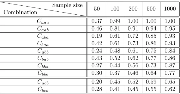
slightly, as is illustrated in table (2). Nevertheless, the spurious phenomenon remains strong.

4 Concluding remarks

We have shown that the spurious regression phenomenon (i.e. diverging t-statistics) in the

estimation of the linear relationship using IV is present when the variables exhibit

nonstatio-nary behaviour (such nonstationarity being deterministic (with a structural break) and/or

stochastic). Moreover, when both the explanatory variable and its instrument are random

(8)

❤❤❤ ❤❤

❤❤ ❤❤

❤❤

Combination

Sample size

50 100 200 500 1000

Caaa 0.37 0.99 1.00 1.00 1.00

Caab 0.46 0.81 0.91 0.94 0.95

Caba 0.19 0.61 0.72 0.85 0.93

Cbaa 0.42 0.61 0.73 0.86 0.93

Cabb 0.24 0.48 0.61 0.75 0.84

Cbab 0.43 0.52 0.62 0.77 0.86

Cbba 0.27 0.44 0.56 0.73 0.87

Cbbb 0.30 0.37 0.46 0.64 0.77

Cacb 0.20 0.45 0.52 0.59 0.65

[image:8.595.184.483.172.329.2]

Cbcb 0.28 0.41 0.45 0.55 0.62

Table 2: Rejection rates of tˆ_δ under autocorrelated innovations

results may complete those obtained in Phillips and Hansen (1990) and Hansen and

Phi-llips (1990); the latter demonstrated that IV is able to provide consistent estimates in a

cointegrated relationship and may actually outperform LS when there is a strong problem

of endogeneity, even if the instruments are spurious. Nevertheless, when there is no

cointe-grated relationship, the reality is that IV provides spurious estimates, just as LS does. The

main result indicates the need for caution with regard to the inferences to be drawn from

IV regression analysis which may in fact be spurious.

A

Proof of Propositions 1 and 2 and Corollary 1

We present a guide as to how to obtain the order in probability of a t-ratio appearing in Proposition (1) in the estimation of regression (1) using IV where the variablesy andxare generated by DGP (3) andz by DGP (2) (all other combinations follow the same steps. Proof of such was provided with the aid ofMathematica 4.1 software6_{) We use the classical}

IV formulas where the number of instruments matches the number of regressors:

ˆ

δIV = (Z′X)−1Z′y

ˆ

σ2 ˆ

δIV = ˆσ

2₍_Z′_X₎−1

(Z′_Z_{) (}_X′_Z₎−1

tˆ_δ_IV = qˆδIV

ˆ

σ2 ˆ

δIV

where,

6

(9)

Z′_X ₌

T Pxt

P

zt Pxtzt

; X′_Z₌

T Pzt

P

xt Pxtzt

; Z′_Z₌

T Pzt

P

zt Pz2t

;

Z′_Y ₌

P

yt

P

ytzt

;

and,

ˆ

σ2=Xyt2+ ˆα2IVT+ ˆδIV2

X

x2t−2ˆαIV

X

yt−2ˆδIV

X

xtyt+ 2ˆαIVδˆIV

X

xt

We shall now describe the process involved in establishing the aforementioned proof. ˆδIV,

ˆ

σ2 ˆ

δIV andtˆδIV are functions of the following expressions (unless indicated otherwise, all sums

(10)

X

wt = W0T+µw

X

t+Xξw,t−1

| {z }

Op

T32

X

zt = µzT+βz

X

t+γz

X

DTzt+

X

uz,t

| {z }

Op T 1 2 X

wt2 = W02T+µ2w

X

t2+Xξw,t2 −1

| {z }

Op(T2)

+2W0µw

X

t

+2W0Xξw,t−1+ 2µw

X

ξw,t−1t

| {z }

Op

T52

X

zt2 = µ2zT+βz2

X

t2+γz2

X

DTzt2 +

X

u2z,t

| {z }

Op(T)

+2µzβz

X

t

+2µzγz

X

DTzt+ 2µz

X

uz,t+ 2βzγz

X

DTztt

+2βz

X

uz,tt

| {z }

Op

T32

+2γz

X

DTztuz,t

| {z }

Op

T32

X

wtzt W0µzT +W0βz

X

t+W0γz

X

DTzt+W0

X

uzt+µwµz

X

t

µwβz

X

t2₊_µ

wγz

X

DTztt+µw

X

uz,tt+µz

X

ξw,t−1

+βz

X

ξw,t−1t+γz

X

DTztξw,t−1

| {z }

Op

T52

+Xξw,t−1uz,t−1

| {z }

Op(T) X

xtyt X0Y0T+X0µy

X

t+X0Xuyt+µxY0

X

t+µxµy

X

t2

+µx

X

uy,tt+Y0

X

ξx,t−1+µy

X

ξx,t−1t+

X

ξx,t−1ξy,t−1

| {z }

Op(T2)

(11)

X

t = 1 2 T

2₊_T

X

t2 = 1 6 2T

3_{+ 3}_T2₊_T

X

DTzt =

1 2

h

T2(1−λz)2+T(1−λz)

i

X

DTzt2 =

1 6

h

2T3(1−λz)3+ 3T2(1−λz)2+T(1−λz)

i

X

DTztt = λzT

X

DTzt+

X

DTzt2

X

DTytDTzt =

X

DTyt2 + (λy−λz)T

X

DTyt

The orders in convergence of the underbraced expressions can be found in Hamilton (1994) pp. 505-506. and in Noriega and Ventosa-Santaularia (2007). The last sum,PDTytDTzt, is

not needed in this example, but it appears in other combinations; we assume, for simplicity, thatλy> λx> λz.

We can fill the previously-cited matrices and then compute the IV parameter estimates and the t-statistic associated with ˆδ. The asymptotics are computed by the program and is represented below. Note that the code provides ˆδLS and ˆσ_δ2ˆ_LS in addition to ˆδIV and ˆσ_δ2ˆ_IV.

To understand it, a brief glossary is required. Letw=x, y, z:

Term Represents Term Represents Term Represents Term Represents

St Pt St2 Pt2

W0 W0 M w µw

Sw Pwt Sw2 Pw

2

t U w

P

uwt U wt Puwtt

U xy Puxtuyt DT xy PDTxtDTyt Ew Pξw,t−1 Ew2 Pξ 2

w,t−1

Ewt Pξw,t−1t Bw βw Gw γw U w2 Pu

2

wt

Sxy Pxtyt M xx X′X−

1

Exy Pξx,t−1ξy,t−1 Exuz Pξx,t−1uzt

DT w PDTwt DT w2 PDT

2

wt DT wt

P_DT

wtt Lw λw

DT zuz PDTztuzt DT zey PDTztξy,t−1 Szey Pztξy,t−1 Szux Pztuxt

[image:11.595.158.450.196.332.2]

Sxz Pxtzt Syz Pytxt Swt Pwtt Sdtxy PDTxyt

Table 3: Glossary of the Mathematica Code

ClearAll; St = 1₂∗(T2₊_T_{); St2 =} 1

6∗(2∗T3+ 3∗T2+T);

ClearAll; St = 1 2∗(T

2₊_T_{); St2 =} 1

6∗(2∗T

3_{+ 3}_∗_T2₊_T_);

ClearAll; St = 1₂∗(T2₊_T_{); St2 =} 1

6∗(2∗T3+ 3∗T2+T);

DTz = 1 2∗(T

2_∗₍₁₋_Lz)2₊_T_∗₍₁₋_Lz));

DTz = 1 2∗(T

2_∗₍₁₋_Lz)2₊_T_∗₍₁₋_Lz));

DTz =1 2∗(T

2_∗₍₁₋_Lz)2₊_T_∗₍₁₋_Lz));

DTz2 = 1

6∗(2∗T

3_∗₍₁₋_Lz)3_{+ 3}_∗_T2_∗₍₁₋_Lz)2₊_T_∗₍₁₋_Lz));

DTz2 =_{DTz2 =}1₆1∗(2∗T3_∗₍₁₋_Lz)3_{+ 3}_∗_T2_∗₍₁₋_Lz)2₊_T_∗₍₁₋_Lz)); 6∗(2∗T

3_∗₍₁₋_Lz)3_{+ 3}_∗_T2_∗₍₁₋_Lz)2₊_T _∗₍₁₋_Lz));

DTzt = DTz2 +T∗Lz∗DTz; DTzt = DTz2 +DTzt = DTz2 +TT∗∗LzLz∗∗DTz;DTz;

Sx = X0∗T+ Mx∗St + Ex∗T32;

Sx = X0Sx = X0∗∗TT+ Mx+ Mx∗∗St + ExSt + Ex∗∗TT32; 3 2;

Sy = Y0∗T+ My∗St + Ey∗T32;

(12)

Sz = Mz∗T+ Bz∗St + Gz∗DTz + Uz∗T12;

Sz = MzSz = Mz∗∗TT+ Bz+ Bz∗∗St + GzSt + Gz∗∗DTz + UzDTz + Uz∗∗TT12; 1 2;

Sx2 = X02∗T+ Mx2∗St2 + Ex2∗T2_{+ 2}_∗_X0_∗_Mx_∗_{St + 2}_∗_X0_∗_Ex_∗_T3 2+

Sx2 = X02∗T + Mx2∗St2 + Ex2∗T2_{+ 2}_∗_X0_∗_Mx_∗_{St + 2}_∗_X0_∗_Ex_∗_T3 2+

Sx2 = X02∗T+ Mx2∗St2 + Ex2∗T2_{+ 2}_∗_X0_∗_Mx_∗_{St + 2}_∗_X0_∗_Ex_∗_T3 2+

2∗Mx∗Ext∗T52;

22∗∗MxMx∗∗ExtExt∗∗TT52; 5 2;

Sy2 = Y02∗T+ My2∗St2 + Ey2∗T2_{+ 2}_∗_Y0_∗_My_∗_{St + 2}_∗_Y0_∗_Ey_∗_T3 2+

Sy2 = Y02∗T + My2∗St2 + Ey2∗T2_{+ 2}_∗_Y0_∗_My_∗_{St + 2}_∗_Y0_∗_Ey_∗_T3 2+

Sy2 = Y02∗T+ My2∗St2 + Ey2∗T2_{+ 2}_∗_Y0_∗_My_∗_{St + 2}_∗_Y0_∗_Ey_∗_T3 2+

2∗My∗Eyt∗T52;

22∗∗MyMy∗∗EytEyt∗∗TT52; 5 2;

Sz2 = Mz2∗T + Bz2∗St2 + Gz2∗DTz2 + Uz2∗T+ 2∗Mz∗Bz∗St+ Sz2 = MzSz2 = Mz22∗∗TT+ Bz+ Bz22∗∗St2 + GzSt2 + Gz22∗∗DTz2 + Uz2DTz2 + Uz2∗∗TT+ 2+ 2∗∗MzMz∗∗BzBz∗∗St+St+ 2∗Mz∗Gz∗DTz + 2∗Mz∗Uz∗T12 + 2∗Bz∗Gz∗DTzt+

22∗∗MzMz∗∗GzGz∗∗DTz + 2DTz + 2∗∗MzMz∗∗UzUz∗∗TT21 + 2∗Bz∗Gz∗DTzt+ 1

2 + 2∗Bz∗Gz∗DTzt+

2∗Bz∗Uzt∗T32 + 2∗Gz∗DTzuz∗T 3 2;

Sxz = X0∗Mz∗T+ X0∗Bz∗St + X0∗Gz∗DTz + X0∗Uz∗T12+

Sxz = X0Sxz = X0∗∗MzMz∗∗TT+ X0+ X0∗∗BzBz∗∗St + X0St + X0∗∗GzGz∗∗DTz + X0DTz + X0∗∗UzUz∗∗TT12+ 1 2+

Mx∗Mz∗St + Mx∗Bz∗St2 + Mx∗Gz∗DTzt + Mx∗Uzt∗T32+

MxMx∗∗MzMz∗∗St + MxSt + Mx∗∗BzBz∗∗St2 + MxSt2 + Mx∗∗GzGz∗∗DTzt + MxDTzt + Mx∗∗UztUzt∗∗TT23+ 3 2+

Mz∗Ex∗T32 + Bz∗Ext∗T 5

2 + Gz∗DTzex∗T 5

2 + Exuz∗T;

Mz∗Ex∗T32+ Bz∗Ext∗T 5

2 + Exuz∗T;

Mz∗Ex∗T32 + Bz∗Ext∗T 5

2 + Exuz∗T;

Syz = Y0∗Mz∗T+ Y0∗Bz∗St + Y0∗Gz∗DTz + Y0∗Uz∗T12+

Syz = Y0Syz = Y0∗∗MzMz∗∗TT+ Y0+ Y0∗∗BzBz∗∗St + Y0St + Y0∗∗GzGz∗∗DTz + Y0DTz + Y0∗∗UzUz∗∗TT12+ 1 2+

My∗Mz∗St + My∗Bz∗St2 + My∗Gz∗DTzt + My∗Uzt∗T32+

MyMy∗∗MzMz∗∗St + MySt + My∗∗BzBz∗∗St2 + MySt2 + My∗∗GzGz∗∗DTzt + MyDTzt + My∗∗UztUzt∗∗TT23+ 3 2+

Mz∗Ey∗T32 + Bz∗Eyt∗T 5

2 + Gz∗DTzey∗T 5

2 + Eyuz∗T;

Mz∗Ey∗T32+ Bz∗Eyt∗T 5

2 + Eyuz∗T;

Mz∗Ey∗T32 + Bz∗Eyt∗T 5

2 + Eyuz∗T;

Sxy = X0∗Y0∗T+ X0∗My∗St + X0∗Ey∗T32 + Y0∗Mx∗St+

Sxy = X0Sxy = X0∗∗Y0Y0∗∗TT+ X0+ X0∗∗MyMy∗∗St + X0St + X0∗∗EyEy∗∗TT23 + Y0∗Mx∗St+ 3

2 + Y0∗Mx∗St+

Mx∗My∗St2 + Mx∗Eyt∗T52+ Y0∗Ex∗T 3

2 + My∗Ext∗T 5

2 + Exy∗T2;

Mx∗My∗St2 + Mx∗Eyt∗T52 + Y0∗Ex∗T 3

2 + My∗Ext∗T 5

2 + Exy∗T2;

Mx∗My∗St2 + Mx∗Eyt∗T52 + Y0∗Ex∗T 3

2 + My∗Ext∗T 5

2 + Exy∗T2;

Mxx = ( T Sx

Sx Sx2 ); Vxy = ( Sy Sxy );

Mxx = ( T Sx

Sx Sx2 ); Vxy = ( Sy Sxy );

Mxx = ( T Sx

Sx Sx2 ); Vxy = ( Sy Sxy ); iMxx = Inverse[Mxx];

iMxx = Inverse[Mxx];iMxx = Inverse[Mxx];

Param1 = iMxx.Vxy; Param1 = iMxxParam1 = iMxx..Vxy;Vxy;

P10 = Factor[Expand[Extract[Param1,{1,1}]]]; P10 = Factor[Expand[Extract[Param1P10 = Factor[Expand[Extract[Param1,,{{11,,11}}]]];]]]; P11num = Numerator[P10];

P11num = Numerator[P10];P11num = Numerator[P10]; K1 = Exponent[P11num, T]; K1 = Exponent[P11numK1 = Exponent[P11num, T, T];];

Anum = Limit[Expand[P11num/TK1_]_{, T} _{→ ∞}_];

Anum = Limit[Expand[P11num_{Anum = Limit[Expand[P11num}/T_/TK1K1_]_]_{, T}_{, T} _{→ ∞}_{→ ∞}_];_];

P12den = Denominator[P10]; P12den = Denominator[P10];P12den = Denominator[P10]; K2 = Exponent[P12den, T]; K2 = Exponent[P12denK2 = Exponent[P12den, T, T];];

Aden = Limit[Expand[P12den/TK2_]_{, T} _{→ ∞}_];

Aden = Limit[Expand[P12den_{Aden = Limit[Expand[P12den}/T_/TK2K2_]_]_{, T}_{, T} _{→ ∞}_{→ ∞}_];_];

Apar = Factor[Expand[(Anum/Aden)∗ TK1

TK2]];

Apar = Factor[Expand[(AnumApar = Factor[Expand[(Anum//Aden)Aden)∗∗TTTK1K2]]; K1

TK2]];

Bnum = Limit[Expand[P21num/TK3_]_{, T} _{→ ∞}_];

Bnum = Limit[Expand[P21num_{Bnum = Limit[Expand[P21num}/T_/TK3K3_]_]_{, T}_{, T} _{→ ∞}_{→ ∞}_];_];

Bden = Limit[Expand[P22den/TK4_]_{, T} _{→ ∞}_];

Bden = Limit[Expand[P22den_{Bden = Limit[Expand[P22den}/T_/TK4K4_]_]_{, T}_{, T} _{→ ∞}_{→ ∞}_];_];

Bpar = Factor[Expand[(Bnum/Bden)∗ TTK3K4]]

Bpar = Factor[Expand[(Bnum/Bden)∗ TK3

TK4]]

Bpar = Factor[Expand[(Bnum/Bden)∗TTK3K4]]

P30 = P30 =P30 = Factor[ Factor[Factor[

Expand[Sy2 + P102∗T + P202∗Sx2−2∗P10∗Sy−2∗P20∗Sxy+ Expand[Sy2 + P10Expand[Sy2 + P1022∗∗TT+ P20+ P2022∗∗Sx2Sx2−−22∗∗P10P10∗∗SySy−−22∗∗P20P20∗∗Sxy+Sxy+ 2∗P10∗P20∗Sx]];

(13)

P31num = Numerator[P30]; P31num = Numerator[P30];P31num = Numerator[P30]; K5 = Exponent[P31num, T]; K5 = Exponent[P31numK5 = Exponent[P31num, T, T];];

Vnum = Factor[Limit[Expand[P31num/TK5_]_{, T} _{→ ∞}_]];

Vnum = Factor[Limit[Expand[P31num_{Vnum = Factor[Limit[Expand[P31num}/T_/TK5K5_]_]_{, T}_{, T} _{→ ∞}_{→ ∞}_]];_]];

Vden = Factor[Limit[Expand[P32den/TK6_]_{, T} _{→ ∞}_]];

Vden = Factor[Limit[Expand[P32den_{Vden = Factor[Limit[Expand[P32den}/T_/TK6K6_]_]_{, T}_{, T} _{→ ∞}_{→ ∞}_]];_]];

Vpar = Factor[Expand[T−1_∗_(Vnum_/_Vden)_∗ TK5

TK6]];

Vpar = Factor[Expand[T−1_∗_(Vnum_/_Vden)_∗ TK5

TK6]];

Vpar = Factor[Expand[T−1_∗_(Vnum_/_Vden)_∗TK5

TK6]];

Varianzas1 = Extract[iMxx,{2,2}]; Varianzas1 = Extract[iMxxVarianzas1 = Extract[iMxx,,{{22,,22}}];];

P40 = Factor[Expand[T−1_∗_P30_∗_{Varianzas1]];}

P40 = Factor[Expand[_{P40 = Factor[Expand[}T_T−−11_∗_∗_P30_P30_∗_∗_{Varianzas1]];}_{Varianzas1]];}

Bvarnum = Limit[Expand[P41num/TK7_]_{, T} _{→ ∞}_];

Bvarnum = Limit[Expand[P41num_{Bvarnum = Limit[Expand[P41num}/T_/TK7K7_]_]_{, T}_{, T} _{→ ∞}_{→ ∞}_];_];

Bvarden = Limit[Expand[P42den/TK8_]_{, T} _{→ ∞}_];

Bvarden = Limit[Expand[P42den_{Bvarden = Limit[Expand[P42den}/T_/TK8K8_]_]_{, T}_{, T} _{→ ∞}_{→ ∞}_];_];

Bvar = Factor[Expand[(Bvarnum/Bvarden)∗TK7

TK8]]

Bvar = Factor[Expand[(BvarnumBvar = Factor[Expand[(Bvarnum//Bvarden)Bvarden)∗∗ TTTK7K8]] K7

TK8]]

Mzx = ( _{Sz Sxz}T Sx ); Mxz = ( _SxT _SxzSz ); Mzz = ( _{Sz Sz2}T Sz );

Mzx = ( T Sx

Sz Sxz ); Mxz = (

T Sz

Sx Sxz ); Mzz = (

T Sz Sz Sz2 ); Mzx = ( _{Sz Sxz}T Sx ); Mxz = ( _SxT _SxzSz ); Mzz = ( _{Sz Sz2}T Sz );

Vzy = ( Sy Syz ); Vzy = ( Sy

Syz ); Vzy = ( Sy

Syz );

iMzx = Inverse[Mzx]; iMxz = Inverse[Mxz]; iMzx = Inverse[Mzx]; iMxz = Inverse[Mxz];iMzx = Inverse[Mzx]; iMxz = Inverse[Mxz];

Param2 = iMzx.Vzy; Param2 = iMzxParam2 = iMzx..Vzy;Vzy;

Fnum = Limit[Expand[P51num/TK9_]_{, T} _{→ ∞}_];

Fnum = Limit[Expand[P51num_{Fnum = Limit[Expand[P51num}/T_/TK9K9_]_]_{, T}_{, T} _{→ ∞}_{→ ∞}_];_];

Fden = Limit[Expand[P52den/TK10_]_{, T} _{→ ∞}_];

Fden = Limit[Expand[P52den_{Fden = Limit[Expand[P52den}/T_/TK10K10_]_]_{, T}_{, T} _{→ ∞}_{→ ∞}_];_];

Fpar = Factor[Expand[(Fnum/Fden)∗ TK9

TK10]];

Fpar = Factor[Expand[(FnumFpar = Factor[Expand[(Fnum//Fden)Fden)∗∗ TTTK10K9]]; K9

TK10]];

Dnum = Limit[Expand[P61num/TK11_]_{, T} _{→ ∞}_];

Dnum = Limit[Expand[P61num_{Dnum = Limit[Expand[P61num}/T_/TK11K11_]_]_{, T}_{, T} _{→ ∞}_{→ ∞}_];_];

Dden = Limit[Expand[P62den/TK12_]_{, T} _{→ ∞}_];

Dden = Limit[Expand[P62den_{Dden = Limit[Expand[P62den}/T_/TK12K12_]_]_{, T}_{, T} _{→ ∞}_{→ ∞}_];_];

Dpar = Factor[Expand[(Dnum/Dden)∗TTK11K12]]

Dpar = Factor[Expand[(Dnum/Dden)∗ TK11

TK12]]

(14)

P70 = P70 =P70 = Factor[ Factor[Factor[

Expand[Sy2 + P502∗T + P602∗Sx2−2∗P50∗Sy−2∗P60∗Sxy+ Expand[Sy2 + P50Expand[Sy2 + P5022∗∗TT+ P60+ P6022∗∗Sx2Sx2−−22∗∗P50P50∗∗SySy−−22∗∗P60P60∗∗Sxy+Sxy+ 2∗P50∗P60∗Sx]];

22∗∗P50P50∗∗P60P60∗∗Sx]];Sx]];

Wnum = Factor[Limit[Expand[P71num/TK13], T → ∞]]; Wnum = Factor[Limit[Expand[P71num_{Wnum = Factor[Limit[Expand[P71num}/T_/TK13K13_]_]_{, T}_{, T} _{→ ∞}_]];

→ ∞]]; P72den = Denominator[P70];

P72den = Denominator[P70];P72den = Denominator[P70]; K14 = Exponent[P72den, T]; K14 = Exponent[P72denK14 = Exponent[P72den, T, T];];

Wden = Factor[Limit[Expand[P72den/TK14_]_{, T} _{→ ∞}_]];

Wden = Factor[Limit[Expand[P72den_{Wden = Factor[Limit[Expand[P72den}/T_/TK14K14_]_]_{, T}_{, T} _{→ ∞}_{→ ∞}_]];_]];

Wpar = Factor[Expand[T−1_∗_(Wnum_/_Wden)_∗ TK13

TK14]];

Wpar = Factor[Expand[T−1_∗_(Wnum_/_Wden)_∗TK13

TK14]];

Wpar = Factor[Expand[T−1_∗_(Wnum_/_Wden)_∗ TK13

TK14]];

Varianzas20 = (iMzx.Mzz.iMxz); Varianzas20 = (iMzxVarianzas20 = (iMzx..MzzMzz..iMxz);iMxz);

Varianzas2 = Extract[Varianzas20,{2,2}]; Varianzas2 = Extract[Varianzas20Varianzas2 = Extract[Varianzas20,,{{22,,22}}];];

P80 = Factor[Expand[T−1_∗_P70_∗_{Varianzas2]];}

P80 = Factor[Expand[_{P80 = Factor[Expand[}T_T−−11_∗_∗_P70_P70_∗_∗_{Varianzas2]];}_{Varianzas2]];}

Dvarnum = Limit[Expand[P81num/TK15_]_{, T} _{→ ∞}_];

Dvarnum = Limit[Expand[P81num_{Dvarnum = Limit[Expand[P81num}/T_/TK15K15_]_]_{, T}_{, T} _{→ ∞}_{→ ∞}_];_];

Dvarden = Limit[Expand[P82den/TK16_]_{, T} _{→ ∞}_];

Dvarden = Limit[Expand[P82den_{Dvarden = Limit[Expand[P82den}/T_/TK16K16_]_]_{, T}_{, T} _{→ ∞}_{→ ∞}_];_];

Dvar = Factor[Expand[(Dvarnum/Dvarden)∗ TTK15K16]]

Dvar = Factor[Expand[(Dvarnum/Dvarden)∗ TK15

TK16]]

Dvar = Factor[Expand[(Dvarnum/Dvarden)∗TTK15K16]]

B

Parameter values of simulations

1. Rejection rates of tˆ_δ_IV under white noise innovations

The values of the parameters in the DGP’s are as follows: all DGP’s: σw = 1 and

no-autocorrelation inuwt. DGP’s with one break: λy = 0.5,λx= 0.3, and λz= 0.6;

γy=−0.015,γx= 0.035, andγz = 0.02. Constants (or drifts): µy= 0.11,µx= 0.09,

andµz= 0.05. Trends: βy= 0.04,βx= 0.07, andβz=−0.07.

2. Rejection rates of tˆ_δ_IV under autocorrelated innovations

all DGP’s are generated as in Table (1) except for the properties of uwt; the

innova-tion processes are generated as AR(1). The values of the parameters in the AR(1) specification are: ρy= 0.5,ρx= 0.4, andρz= 0.7

References

Entorf, H.(1997): “Random walks with drifts: Nonsense regression and spurious fixed-effect estimation,” Journal of Econometrics, 80(2), 287–296.

Hamilton, J.(1994): Time Series Analysis. Princeton University Press.

(15)

Hasseler, U. (2000): “Simple Regressions with Linear Time Trends,” Journal of Time Series Analysis, 21, 27–32.

Kim, T., S. Lee, and P. Newbold(2004): “Spurious Regressions With Stationary Pro-cesses Around Linear Trends,”Economics Letters, 83, 257–262.

Marmol, F. (1995): “Spurious Regression Between I (d) Processes,” Journal of Time Series Analysis, 16, 313–321.

(1998): “Spurious regression theory with nonstationary fractionally integrated processes,” Journal of Econometrics, 84(2), 233–250.

Morgan, M.(1992): The History of Econometric Ideas. Cambridge University Press.

Noriega, A.,andD. Ventosa-Santaul`aria(2006): “Spurious Regression Under Broken Trend Stationarity,”Journal of Time Series Analysis, 27, 671–684.

Noriega, A.,andD. Ventosa-Santaularia(2007): “Spurious Regression and Trending Variables,”Oxford Bulletin of Economics and Statistics, 69(3), 439–444.

Perron, P., and X. Zhu (2005): “Structural breaks with deterministic and stochastic trends,” Journal of Econometrics, 129(1-2), 65–119.

Phillips, P. (1986): “Understanding Spurious Regressions in Econometrics,” Journal of Econometrics, 33(3), 311–40.

Phillips, P., and B. Hansen (1990): “Statistical Inference in Instrumental Variables Regression with I (1) Processes,”The Review of Economic Studies, 57(1), 99–125.